
Local Performance of the (μ/μI, λ)-ES in a Noisy Environment
Dirk V. Arnold [email protected]; Hans-Georg Beyer [email protected] Department of Computer Science XI University of Dortmund 44221 Dortmund, Germany
Abstract
While noise is a phenomenon present in many real-world optimization problems, the understanding of its potential effects on the performance of evolutionary algorithms is still incomplete. In the realm of evolution strategies in particular, it can frequently be observed that one-parent strategies are outperformed by multi-parent strategies in noisy environments. However, mathematical analyses of the performance of evolution strategies in noisy environments have so far been restricted to the simpler one-parent strategies.
This paper investigates the local performance of a multi-parent evolution strategy employing intermediate multi-recombination on a noisy sphere in the limit of infinite parameter space dimension. The performance law that is derived neatly generalizes a number of previously obtained results. Genetic repair is shown to be present and unaffected by the noise. In contrast to previous findings in a noise-free environment, the efficiency of the simple (l+1)-ES can be exceeded by multi-parent strategies in the presence of noise. It is demonstrated that a much improved performance as compared to one-parent strategies can be achieved. For large population sizes the effects of noise all but vanish.
1 INTRODUCTION
Noise is a common phenomenon in many real-world optimization problems. It can stem from sources as different as errors of measurement in experiments, from the use of stochastic sampling or simulation procedures, or from interactions with users, to name but a few. Reduced convergence velocity or even inability to approach the optimum are commonly observed consequences of the presence of noise on optimization strategies.
It can frequently be observed in experiments that evolutionary algorithms (EAs) are comparatively robust with regard to the effects of noise. In fact, noisy environments are considered to be a prime area for the application of EAs. For genetic algorithms (GA), optimization in noisy environments has been investigated, among others, by Fitzpatrick and Grefenstette [10], Miller and Goldberg [12], and Rattray and Shapiro [15]. Their work has led to recommendations regarding population sizing and the use of resampling, and it has been shown that in the limit of an infinitely large population the effects of noise on the performance of a GA employing Boltzmann selection are entirely removed.
In the realm of evolution strategies (ESs), theoretical studies of the effects of noise date back to early work of Rechenberg [16] who analyzed the performance of a (1 + 1)-ES in a noisy corridor. An analysis of the performance of the (1 + A)-ES on a noisy sphere by Beyer [3] sparked empirical research by Hammel and Bäck [11] who concluded that the findings made for GAs do not always easily translate to ES. Arnold and Beyer [2] address the effects of overvaluation of the parental fitness using a (1 + 1)-ES on a noisy sphere. Both Rechenberg [17] and Beyer [7, 8] give results regarding rescaled mutations in (1, λ)- ES. For an overview of the status quo of ES research concerned with noisy environments and for additional references see [1, 8].
Empirical evidence presented by Rechenberg [17] and by Nissen and Propach [13] as well as by a number of others suggests that population-based optimization methods are generally superior to point-based methods in noisy environments. However, analytically obtained results in the field of ES have been published only for single-parent strategies. The present paper attempts to close part of this gap between theory and empirical observations by presenting a formal analysis of the local performance of a (μ/μI, λ)-ES on a noisy sphere in the limit of infinite parameter space dimensionality. The results of the analysis can serve as an approximation for large but finite parameter space dimensionality provided that population sizes are chosen not too large.
Much of the theoretically-oriented research on ES relies on the examination of the local behavior of the strategies in very simple fitness environments. While such environments bear only little resemblance to real-world problems, they have the advantage of mathematical tractability. Frequently, consideration of simple fitness environments, such as the sphere or the ridge, leads to an understanding of working mechanisms of ES that can explain phenomena observable or be of practical use in more complex fitness environments. The discovery of the genetic repair principle [5] and the recommendation regarding the sizing of the learning parameter in self-adaptive strategies in [19] are but two examples. The present paper continues this line of research by analyzing the behavior of the (μ/μI, λ)-ES on a sphere with fitness measurements disturbed by Gaussian noise. The results derived are accurate in the limit of an infinite-dimensional parameter space and can serve as approximations for large but finite-dimensional parameter spaces.
This paper is organized as follows. Section 2 outlines the (μ/μI, λ)-ES algorithm and the fitness environment for which its performance will be analyzed. The notion of fitness noise is introduced. In Section 3, a local performance measure – the expected fitness gain from one generation to the next – is computed. It is argued that for the spherically symmetric environment that is investigated, in the limit of an infinite-dimensional parameter space the expected fitness gain formally agrees with the progress rate. Section 4 discusses the results. It is demonstrated that the performance gain as compared with one-parent strategies is present for small population sizes already. It is shown that in contrast to the noise-free situation, the efficiency of the (1 + 1)-ES can be exceeded by that of a (μ/μI, λ)-ES if noise is present. Section 5 concludes with a brief summary and suggestions for future research.
2 ALGORITHM AND FITNESS ENVIRONMENT
Section 2.1 describes the (μ/μI, λ)-ES with isotropic normal mutations applied to optimization problems with a fitness function of the form f: ![]() N →
N → ![]() . Without loss of generality, it can be assumed that the task at hand is minimization, i.e. that high values of f correspond to low fitness and vice versa. Section 2.2 outlines the fitness environment for which the performance of the algorithm is analyzed in the succeeding sections.
. Without loss of generality, it can be assumed that the task at hand is minimization, i.e. that high values of f correspond to low fitness and vice versa. Section 2.2 outlines the fitness environment for which the performance of the algorithm is analyzed in the succeeding sections.
2.1 THE (μ/μI, λ)-ES
As an evolutionary algorithm, the(μ/μI, λ)-ES strives to drive a population of candidate solutions to an optimization problem towards increasingly better regions of the search space by means of variation and selection. The parameters λ and μ refer to the number of candidate solutions generated per time step and the number of those retained after selection, respectively. Obviously, λ is also the number of fitness function evaluations required per time step.
Selection simply consists in retaining the μ best of the candidate solutions and discarding the remaining ones. The comma in (μ/μ, λ) indicates that the set of candidate solutions to choose from consists only of the λ offspring, whereas a plus would indicate that selection is from the union of the set of offspring and the parental population. As shown in [2], plus-selection in noisy environments introduces overvaluation as an additional factor to consider, thus rendering the analysis considerably more complicated. Moreover, as detailed by Schwefel [19], comma-selection is known to be preferable if the strategy employs mutative self-adaptation of the mutation strength, making it the more interesting variant to consider.
Variation is accomplished by means of recombination and mutation. As indicated by the second μ and the subscript I in (μ/μ, λ), recombination is “global intermediate”. More specifically, let x(t) ∈ ![]() N, i = 1,…, μ, be the parameter space locations of the parent individuals. Recombination consists in computing the centroid
N, i = 1,…, μ, be the parameter space locations of the parent individuals. Recombination consists in computing the centroid
〈x〉=1μμ∑t=1x(t)
![]()
of the parental population. Mutations are isotropically normal. For every descendant y(j) ∈ ![]() N, j = 1,…, λ, a mutation vector z(j) = 1,…, λ, which consists of N independent, normally distributed components with mean 0 and variance σ2, is generated and added to the centroid of the parental population. That is,
N, j = 1,…, λ, a mutation vector z(j) = 1,…, λ, which consists of N independent, normally distributed components with mean 0 and variance σ2, is generated and added to the centroid of the parental population. That is,
y(j)=〈x〉+z(j)
![]()
The standard deviation σ of the components of the mutation vectors is referred to as the mutation strength.
The fitness advantage associated with a mutation z applied to search space location x is defined as
qx(z)=f(x)−f(x+z).
For a fixed location x in parameter space, qx is a scalar random variate with a distribution that depends both on the fitness function and on the mutation strength.
The local performance of the algorithm can be measured either in parameter space or in terms of fitness. The corresponding performance measures are the progress rate φ and the expected fitness gain q, respectively. The expected fitness gain is the expected difference in fitness between the centroids of the population at consecutive time steps. That is, letting 〈x〉(g) denote the centroid of the parental population at generation g, the expected fitness gain is the expected value of f(〈x〉(g))−f(〈x〉(g+`))![]() . The progress rate is the expected distance in parameter space in direction of the location of the optimum covered by the population’s centroid from one generation to the next. That is, letting R(g) denote the Euclidean distance between the centroid of the parental population and the optimum of the fitness function, the progress rate is the expected value of R(g) – R(g + 1). For the fitness environment outlined in Section 2.2 the two performance measures coincide in the limit N → ∞ if appropriately normalized as will be seen in Section 3.
. The progress rate is the expected distance in parameter space in direction of the location of the optimum covered by the population’s centroid from one generation to the next. That is, letting R(g) denote the Euclidean distance between the centroid of the parental population and the optimum of the fitness function, the progress rate is the expected value of R(g) – R(g + 1). For the fitness environment outlined in Section 2.2 the two performance measures coincide in the limit N → ∞ if appropriately normalized as will be seen in Section 3.
2.2 THE FITNESS ENVIRONMENT
Computing the expected fitness gain is a hopeless task for all but the most simple fitness functions. In ES theory, a repertoire of fitness functions simple enough to be amenable to mathematical analysis while at the same time interesting enough to yield non-trivial results and insights has been established [4, 14]. The most commonplace of these fitness functions is the quadratic sphere
f(x)=N∑t=1(ˆxt−xt)2,
![]()
where x = (x1,…, xN)T is the location in parameter space of the optimal fitness value. This fitness function simply maps points in ![]() N to the square of their Euclidean distance to the optimum at ˆx
N to the square of their Euclidean distance to the optimum at ˆx![]() . By formally letting the parameter space dimension N tend to infinity and introducing appropriate normalizations as defined below, a number of simplifying conditions hold true. Note that often results that have been obtained for the sphere can be extended to more general situations. Rudolph [18] derives bounds for the performance of ES for arbitrary convex fitness functions. Beyer [4] presents a differential geometric approach that locally approximates arbitrary fitness functions and presents a fitness gain theory that applies to general quadratic fitness functions.
. By formally letting the parameter space dimension N tend to infinity and introducing appropriate normalizations as defined below, a number of simplifying conditions hold true. Note that often results that have been obtained for the sphere can be extended to more general situations. Rudolph [18] derives bounds for the performance of ES for arbitrary convex fitness functions. Beyer [4] presents a differential geometric approach that locally approximates arbitrary fitness functions and presents a fitness gain theory that applies to general quadratic fitness functions.
In what follows it is assumed that there is noise involved in the process of evaluating the fitness function. This form of noise has therefore been termed fitness noise. Loosely speaking, it deceives the selection mechanism. An individual at parameter space location x has an ideal fitness f(x) and a perceived fitness that may differ from its ideal fitness. Fitness noise is commonly modeled by means of an additive, normally distributed random term with mean zero. That is, in a noisy environment, evaluation of the fitness function at parameter space location x yields perceived fitness f(x) + σ![]() δ, where δ is a standard normally distributed random variate. Quite naturally, σ
δ, where δ is a standard normally distributed random variate. Quite naturally, σ![]() is referred to as the noise strength and may depend on the parameter space location x.
is referred to as the noise strength and may depend on the parameter space location x.
3 PERFORMANCE
This section computes the expected fitness gain, or, equivalently, the progress rate, for the (μ/μ, λ)-ES in the environment outlined in Section 2.2. It relies on a decomposition of mutation vectors suggested in both [3] and in [17] and is illustrated in Figure 1. A mutation vector z originating at parameter space location x can be written as the sum of two vectors zA and zB, where zA is parallel to ˆx−x![]() and zB is in the hyper-plane perpendicular to that. Due to the isotropy of mutations, it can without loss of generality be assumed that zA = σ(z1,0,…, 0)T and zB = σ(0, z2,…, zN)T, where the zt, I,…, N, are independent, standard normally distributed random variates and σ is the mutation strength. Using elementary geometry and denoting the respective distances of x and of y = x + z to the location of the optimum by R and r, respectively, it can be seen from Figure 1 that
and zB is in the hyper-plane perpendicular to that. Due to the isotropy of mutations, it can without loss of generality be assumed that zA = σ(z1,0,…, 0)T and zB = σ(0, z2,…, zN)T, where the zt, I,…, N, are independent, standard normally distributed random variates and σ is the mutation strength. Using elementary geometry and denoting the respective distances of x and of y = x + z to the location of the optimum by R and r, respectively, it can be seen from Figure 1 that
r2=(R−σz1)2+||zB||2=R2−2Rσz1+σ2z21+σ2N∑i=2z21
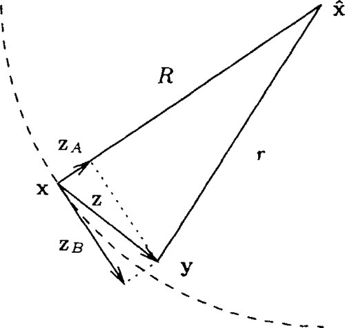
 , vector zB is in the hyper-plane perpendicular to that. The starting and end points, x and y, of the mutation are at distances R and r, respectively, from the location of the optimum.
Introducing normalized quantities
σ*=σNR,σ*ε=σεN2R2andq*x(z)=qx(z)N2R2,
![]()
the normalized fitness advantage associated with mutation vector z from Equation (1) is thus
q*(z)=N2R2(R2−r2)=σ*z1−σ*22Nz21−σ*22NN∑1=2z21
Note that the index x of the normalized fitness advantage has been dropped as the normalized fitness advantage is independent of the location in parameter space due to the choice of normalizations.
The second summand on the right hand side of Equation (3) can for large N with overwhelming probability be neglected compared to the third summand. The term ∑Nt=2z2t/N contained in the third summand on the right hand side of Equation (3) is according to the Central Limit Theorem of Statistics asymptotically normal with mean (N – 1)/N ≈ 1 and variance 2(N – 1)/N2 ≈ 2/N. In the limit N → ∞, the third summand and therefore the contribution of the zB component to the fitness advantage is thus simply −σ*2/2
![]() . Note that the components zt, i = 2, …, N of the mutation vector do not influence the fitness advantage associated with a mutation as for large enough N they statistically average out. Thus, the Zi, i = 2, …, N, are selectively neutral and for large N the fitness advantage associated with mutation vector z can be approximated as
. Note that the components zt, i = 2, …, N of the mutation vector do not influence the fitness advantage associated with a mutation as for large enough N they statistically average out. Thus, the Zi, i = 2, …, N, are selectively neutral and for large N the fitness advantage associated with mutation vector z can be approximated as
q*(z)≈σ*z1−σ*22.
As shown in Appendix A this relation is exact in the limit N → ∞.
Selection is performed on the basis of perceived fitness rather than ideal fitness. With the definition of fitness noise from Section 2.2, the perceived normalized fitness advantage associated with mutation vector z in the limit N → ∞ is
q*(z)+σ*εδ=σ*(z1+ϑδ)−σ*22,
where δ is a standard normal random variate and ϑ=σ*ε/σ*![]() is the noise-to-signal ratio. Those μ offspring individuals with the highest perceived fitness are selected to form the parental population of the succeeding time step. Let (k; λ), k = 1,…, λ, be the index of the offspring individual with the kth highest perceived fitness. The difference between the parameter space location of the centroid of the selected offspring and the centroid of the parental population of the present time step is the progress vector
is the noise-to-signal ratio. Those μ offspring individuals with the highest perceived fitness are selected to form the parental population of the succeeding time step. Let (k; λ), k = 1,…, λ, be the index of the offspring individual with the kth highest perceived fitness. The difference between the parameter space location of the centroid of the selected offspring and the centroid of the parental population of the present time step is the progress vector
〈z〉=1μμ∑k=`z(k;λ),
![]()
which consists of components 〈zi〉=∑μk=11zt(k;λ)/μ. The expected fitness gain of the strategy is the expected value of the fitness advantage
q*(〈z〉)=σ*(z1)−σ*22N〈z1〉2−σ*22NN∑t=2〈zt〉2
associated with this vector.
The vector 〈z〉 can be decomposed into two components 〈zA〉 and 〈zB〉 in very much the same manner as shown above and as illustrated in Figure 1 for mutation vectors. As the zB components of mutation vectors are selectively neutral, the zB components of the mutation vectors that are averaged are independent. Therefore, each of the 〈zi〉, I = 2,…, N, is normal with mean 0 and variance 1/μ. Following the line of argument outlined in the derivation leading to Equation (4), the contribution of the zB components to the expected fitness gain is thus –σ*2/2 μ. Note the occurence of the factor μ in the denominator that reflects the presence of genetic repair, the influence that has in [5] been found to be responsible for the improved performance of the (μ/μI, λ)-ESas compared with the (1, λ)-ES.
We now argue that the second summand on the right hand side of Equation (6) can be neglected compared with the third provided that N is large enough. This is the case if μ〈z1〉2≪N![]() . Assume that A is fixed and finite. The value of 〈z1〉2 is independent of N. Its mean is not greater than the square of the average of the first μ order statistics of λ independent, standard normally distributed random variables. Therefore, for any
. Assume that A is fixed and finite. The value of 〈z1〉2 is independent of N. Its mean is not greater than the square of the average of the first μ order statistics of λ independent, standard normally distributed random variables. Therefore, for any ![]() > 0 an N can be given such that the probability that μ〈z1〉2≪N
> 0 an N can be given such that the probability that μ〈z1〉2≪N![]() does not hold is less than
does not hold is less than ![]() . As a consequence, the second summand can be neglected.
. As a consequence, the second summand can be neglected.
Computing the expected value of the first summand on the right hand side of Equation (6) is technically involved but straightforward. The calculations are referred to Appendix B. Denoting the cumulative distribution function of the standard normal distribution by Φ and following [5] in defining the (μ/μ, λ)-progress coefficient as
cμ/μ,λ=λ−μ2π(λμ)∫∞−∞e−x2[Φ(x)]λ−μ−1[1−Φ(x)]μ−1dx,
the result arrived at in Equation (13) reads
¯〈z1〉=cμ/μ,λ√1+ϑ2
Therefore, the expected fitness gain of the (μ/μI, λ)-ES on the noisy, infinite-dimensional quadratic sphere is
ˉq*=cμ/μ,λσ*√1+ϑ2−σ*22μ
The relevance of this result is discussed in Section 4.
We now make plausible that this result formally agrees with the result for the normalized progress rate, i.e. that in the limit N → ∞ the progress rate law
φ*=cμ/μ,λσ*√1+ϑ2−σ*22μ,
where φ* is the expected value of N(R – r)R, holds. For finite normalized mutation strength the normalized fitness gain is finite. Therefore, with increasing N the expected value of the difference between the distance R of the parental centroid from the location of the optimum and the distance r of the centroid of the selected offspring to the location of the optimum tends to zero. As
NR2−r22R2=NR−rR⋅R+r2R,
and as (R + r)/2R tends to one, it follows that Equation (9) holds.
4 DISCUSSION
Equation (9) generalizes several previously obtained results and confirms a number of previously made hypotheses and observations. In particular, for σ*ε=0,![]() Equation (9) agrees formally with the result of the progress rate analysis of the (μ/μI, λ)-ES on the noise-free sphere published in [5]. For μ = 1, results of the analysis of the (1, λ)-ES on the noisy sphere that have been derived in [3] and [17] appear as special cases. Moreover, solving Equation (9) for the distance to the optimum R proves the validity of a hypothesis regarding the residual location error made in [8]. Finally, Equation (9) confirms empirical findings regarding the performance of the (μ/μI, λ)-ES made by Herdy that are quoted in [17].
Equation (9) agrees formally with the result of the progress rate analysis of the (μ/μI, λ)-ES on the noise-free sphere published in [5]. For μ = 1, results of the analysis of the (1, λ)-ES on the noisy sphere that have been derived in [3] and [17] appear as special cases. Moreover, solving Equation (9) for the distance to the optimum R proves the validity of a hypothesis regarding the residual location error made in [8]. Finally, Equation (9) confirms empirical findings regarding the performance of the (μ/μI, λ)-ES made by Herdy that are quoted in [17].
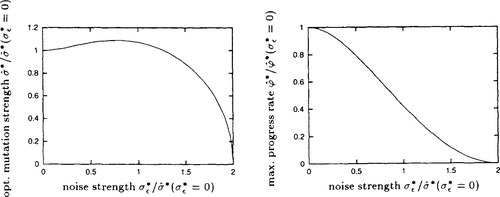
Figure 2 is obtained by numerically solving Equation (9) for the normalized mutation strength ˆσ*![]() that maximizes the normalized progress rate. Throughout this section, this mutation strength is considered optimal. Both the optimal normalized mutation strength and the resulting normalized progress rate are shown as functions of the normalized noise strength. Note that the axes are scaled by dividing by the optimal normalized mutation strength ˆσ*(σ*ε=0)=μcμ/μ,λ
that maximizes the normalized progress rate. Throughout this section, this mutation strength is considered optimal. Both the optimal normalized mutation strength and the resulting normalized progress rate are shown as functions of the normalized noise strength. Note that the axes are scaled by dividing by the optimal normalized mutation strength ˆσ*(σ*ε=0)=μcμ/μ,λ![]() in the absence of noise for normalized noise strength and normalized mutation strength and by the maximal normalized progress rate ˆσ*(σ*ε=0)=μc2μ/μ/λ/2
in the absence of noise for normalized noise strength and normalized mutation strength and by the maximal normalized progress rate ˆσ*(σ*ε=0)=μc2μ/μ/λ/2![]() in the absence of noise for the normalized progress rate. Using the scaled quantities the resulting graphs are independent of the population size parameters. For the noisy (1, λ)-ES the figure can already be found in [17].
in the absence of noise for the normalized progress rate. Using the scaled quantities the resulting graphs are independent of the population size parameters. For the noisy (1, λ)-ES the figure can already be found in [17].
 and maximal progress rate ⌢φ*
 as functions of normalized noise strength σε* Note the scaling of the axes: normalized mutation strength and normalized progress rate are scaled by their respective optimal values in the absence of noise; the normalized noise strength is scaled by the optimal normalized mutation strength in the absence of noise.
It can be seen from Figure 2 that a (1, λ)-ES is capable of progress up to a normalized noise strength of σ*ε=2c1,λ,![]() while a, (μ/μI, λ)-ES is capable of progress up to a normalized noise strength of 2μcμ/μ,λ. That is, a positive progress rate can be achieved for any noise strength by increasing the population size. The reason for this improved performance is – as in the absence of noise – the genetic repair effect. Genetic repair acts in the noisy environment as it does in the noise-free one: the components of the mutation vectors that do not lead towards the optimum but away from it are reduced by the averaging effect of recombination as signified by the presence of the factor μ in the denominator of the loss term in Equation (9). As a consequence, it is possible to explore the search space at higher mutation strengths. In a noisy environment, these increased mutation strengths have the additional benefit of leading to a reduced noise-to-signal ratio ϑ that in limit of very large population sizes tends to zero. Note however that care is in place here as finite population sizes had to be assumed in the limiting process N → ∞. Therefore, no statements regarding the limiting case μ → ∞ can be made. A performance analysis of the (μ/μI, λ)-ES in finite-dimensional search spaces will be necessary to arrive at conclusive statements regarding the behavior of strategies employing very large populations or to obtain conclusive results in rather low dimensional search spaces.
while a, (μ/μI, λ)-ES is capable of progress up to a normalized noise strength of 2μcμ/μ,λ. That is, a positive progress rate can be achieved for any noise strength by increasing the population size. The reason for this improved performance is – as in the absence of noise – the genetic repair effect. Genetic repair acts in the noisy environment as it does in the noise-free one: the components of the mutation vectors that do not lead towards the optimum but away from it are reduced by the averaging effect of recombination as signified by the presence of the factor μ in the denominator of the loss term in Equation (9). As a consequence, it is possible to explore the search space at higher mutation strengths. In a noisy environment, these increased mutation strengths have the additional benefit of leading to a reduced noise-to-signal ratio ϑ that in limit of very large population sizes tends to zero. Note however that care is in place here as finite population sizes had to be assumed in the limiting process N → ∞. Therefore, no statements regarding the limiting case μ → ∞ can be made. A performance analysis of the (μ/μI, λ)-ES in finite-dimensional search spaces will be necessary to arrive at conclusive statements regarding the behavior of strategies employing very large populations or to obtain conclusive results in rather low dimensional search spaces.
The benefit of increased mutation strengths in noisy environments has been recognized before and has led to the formulation of (1, λ)-ES using rescaled mutations in [17, 7, 8]. The present analysis shows that the positive effect of an increased mutation strength can naturally be achieved in (μ/μI, λ)-ES, and that no rescaling is required. However, this does not solve the problems related to mutation strength adaptation of (1, λ)-ES using rescaled mutations pointed out in [8] as the self-adaptation of mutation strengths in (μ/μI, λ)-ES does not work optimally either.
Defining the efficiency η of an ES as the expected normalized fitness gain, or equivalently the normalized progress rate, per fitness function evaluation for optimally chosen mutation strength, Beyer [6] has shown that on the sphere in the absence of noise, the efficiency of the (l-t-l)-ES cannot be exceeded by any (μ/μI, λ)-ES but only asymptotically be reached for very large population sizes. This is not so in noisy environments. Figure 3a) shows the number of offspring per generation λ above which an optimally adjusted (μ/μI, λ)-ES outperforms an optimally adjusted (1 + 1)-ES on the infinite-dimensional noisy sphere. It has been obtained by numerically comparing the efficiency of the (μ/μI, λ)-ES that follows from dividing the normalized progress rate φ* in Equation (9) by λ with the normalized progress rate of the (1 + 1)-ES computed in [2]. It can be seen that the efficiency of the (1 + 1)-ES can be exceeded even for moderate population sizes if there is noise present. For example, for normalized noise strengths above about 0.59, a (2/2I, 6)-ES can be more efficient than a (1 + 1)-ES. Only for relatively small normalized noise strengths below 0.2 are large population sizes required to outperform the (1 + 1)-ES. This is a strong point in favor of the use of multi-parent rather than single-parent optimization strategies in noisy environments.
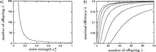
 of the μ/μI, λ)-ES with optimally chosen number of parents μ as a function of the number of offspring λ. The lines correspond to, from top to bottom, normalized noise strengths σε* = 0.0. 1.0, 2.0, 4.0, 8.0, and 16.0.
Figure 3b) shows the efficiency of (μ/μI, λ)-ES with optimally chosen parameter μ as a function of the number of offspring per generation λ for a number of noise levels. It has been obtained by numerically optimizing the efficiency while considering μ as a real valued parameter in order to smoothen the curves. It can be seen from the asymptotic behavior of each line in the figure that by sufficiently increasing the population size the efficiency can be increased up to its maximal value of 0.202 in the absence of noise. However, it is once more stressed that the relevance of this result for finite-dimensional parameter spaces is rather limited.
5 CONCLUSION
To conclude, the local performance of the (μ/μI, λ)-ES on the noisy, infinite-dimensional quadratic sphere has been analyzed. It has been shown that by increasing the population size the effects of noise can be entirely removed. This theoretical result seems to support the validity for ES of empirical observations made by Fitzpatrick and Grefenstette [10] for GAs. For (μ/μI, λ)-ES the improved performance is due to genetic repair which makes it possible to use increased mutation strengths and thereby to decrease the noise-to-signal ratio. It has also been demonstrated that, in contrast to the noise-free case, the efficiency of the (1 + 1)-ES can be exceeded by a multi-parent strategy employing recombination, and that even for relatively moderate noise strengths rather small population sizes are sufficient to achieve this.
Future work includes analyzing the performance of the (μ/μI, λ)-ES in other fitness environments and extending the analysis to strategies employing dominant rather than intermediate recombination by means of surrogate mutations as exemplified for noise-free environments in [17, 5]. Of particular interest is the extension of the analysis presented here to finite-dimensional parameter spaces. Furthermore, the analysis of the performance of ES employing no recombination or recombination with fewer than μ parents remains as a challenge for the future. The results of such an analysis may prove to be of particular interest as empirical results quoted in [17] indicate that performance improvements not accounted for by the present theory can be observed. Finally, an investigation of the effects of noise on the behavior of mutation strength adaptation schemes such as mutative self-adaptation is of great interest as such schemes are an essential ingredient of ES.
APPENDIX A: SHOWING THE ASYMPTOTIC NORMALITY OF THE FITNESS ADVANTAGE ASSOCIATED WITH A MUTATION VECTOR
The goal of this appendix is to formally show that in the limit N → ∞ the distribution of the normalized fitness advantage is normal with mean – σ*2/2 and variance σ*2. Let
f1(z1)=σ*z1−σ*22Nz2I
![]()
and
f2(z2,…,zN)=−σ*22NN∑t=2z2t.
Then q*(z) = f1(z1) + f2(z2, …, zN) and the characteristic function of q*(z) is the product of the characteristic functions of f1(z1) and f2(z2,…,zN) due to the independence of the summands.
The characteristic function of f2(z2,…, zN) is easily determined. As the sum ∑Nt=2z2i![]() is χ2N−1
is χ2N−1![]() -distributed, the charateristic function of f2(z2,…, zN) is
-distributed, the charateristic function of f2(z2,…, zN) is
ϕ2(t)=(1+σ*2Nit)−12(N−1)
where i denotes the imaginary unit.
The characteristic function of f1(z1) is not as easily obtained. It can be verified that for y ≤ N/2
f1(z1)<y⇔z1<Nσ*[1−√1−2yN]orz1>Nσ*[1+√1−2yN]
![]()
and that f1(z1) < y with probability 1.0 if y > N/2. Recall that z1 is standard normally distributed. Let
Φ(x)=1√2π∫x−∞e−12t2dt
denote the cumulative distribution function of the standard normal distribution. The cumulative distribution function of f1(z1) is then
P1(y)={1Φ(Nσ*(1−√1−2yN))+1−Φ(Nσ*(1+√1−2yN))ify≥N/2ify<N/2
The corresponding probability density function
p1(y)={01√2πσ*√1−2y/N[exp(−N22σ*2(1−√1−2yN)2)+exp(−N22σ*2(1+√1−2yN)2)]ify≥N/2ify<N/2
is obtained by differentiation. Using substitution z=√1−2y/N![]() it follows
it follows
ϕ1(t)=∫∞−∞p1(y)eitydy=N√2πσ*∫∞0[exp(−N2(1−z)22σ*2)+exp(−N2(1+z)22σ*2)]exp(itN2(1−z2))dz=1√1+σ*2it/Nexp(−12σ*2t21+σ*2it/N).
for the characteristic function of f1(z1), where the final step can be verified using an algebraic manipulation system.
Thus, overall the characteristic function of q*(z) is
ϕ(t)=ϕ1(t)ϕ2(t)=1(1+σ*2it/N)N/2exp(−12σ*2t21+σ*2it/N).
We now use a property that Stuart and Ord [20] refer to as The Converse of the First Limit Theorem on characteristic functions: If a sequence of characteristic functions converges to some characteristic function everywhere in its parameter space, then the corresponding sequence of distribution functions tends to a distribution function that corresponds to that characteristic function. Due to the relationship
limN→∞1(1+x/N)N/2=exp(−x2),
the first factor on the right hand side of Equation (10) tends to exp(–σ*2 it/2). The second factor tends to exp(–σ*2 t2/2). Therefore, it follows that for any t
limN→∞ϕ(t)=exp(1σ*22(t2+it)).
As this is the characteristic function of a normal distribution with mean –σ*2/2 and variance σ*2 the asymptotic normality of the fitness advantage has been shown.
APPENDIX B COMPUTING THE MEAN OF 〈z1〉
Let z1(t) and δ(i), i = 1, …, λ, be independent standard normally distributed random variables. Let (k; λ) denote the index with the kth largest value of z1(i) + ϑδ(t) The goal of this appendix is to compute the expected value of the average
〈z1〉=1μμ∑k=1z(k;λ)1,
of those μ of the z1(i) that have the largest values of z(i)1+ϑδ(i)![]() .
.
Denoting the probability density function of z1(k; λ) as Pk;λ, the expected value can be written as
¯〈z1〉=1μμ∑k=1∫∞−∞xpk;λ(x)dx.
Determining the density pk;λ requires the use of order statistics. The z1(i) have standard normal density. The terms z(t)1+ϑδ(t)![]() are independently normally distributed with mean 0 and variance 1 + ϑ2. The value of z(t)1+ϑδ(t)
are independently normally distributed with mean 0 and variance 1 + ϑ2. The value of z(t)1+ϑδ(t)![]() is for given z(i)1=x
is for given z(i)1=x![]() normally distributed with mean x and variance ϑ2. For an index to have the kth largest value of z(t)1+ϑδ(t)
normally distributed with mean x and variance ϑ2. For an index to have the kth largest value of z(t)1+ϑδ(t)![]() , k – 1 of the indices must have larger values of z(t)1+ϑδ(t)
, k – 1 of the indices must have larger values of z(t)1+ϑδ(t)![]() and λ – k must have smaller values of z(t)1+ϑδ(t)
and λ – k must have smaller values of z(t)1+ϑδ(t)![]() As there are λ times k – 1 out of λ – 1 different such cases, it follows
As there are λ times k – 1 out of λ – 1 different such cases, it follows
pk;λ(x)=12πϑλ!(λ−k)!(k−1)!e−12x2∫∞−∞exp(−12(y−xϑ)2)[Φ(y√1+ϑ2)]λ−k[1−Φ(y√1+ϑ2)]k−1dy

for the density of zk;λ
Inserting Equation (12) into Equation (11) and swapping the order of integration and summation it follows
¯〈z1〉=12πμϑ∫∞−∞xe−12x2∫∞−∞exp(−12(y−xϑ)2)μ∑k=1λ!(λ−k)!(k−1)![Φ(y√1+ϑ2)]λ−k[1−Φ(y√1+ϑ2)]k−1dydx.

Using the identity (compare [6], Equation (5.14))
μ∑k=1λ!(λ−k)!(k−1)!Pλ−k[1−P]k−1=λ!(λ−μ−1)!(μ−1)!∫P0zλ−μ−1[1−z]μ−1dz
it follows
¯〈z1〉=λ−μ2πϑ(λμ)∫∞−∞xe−12x2∫∞−∞exp(−12(y−xϑ)2)∫Φ(y/√1+ϑ2)0zλ−μ−1[1−z]μ−1dzdydx.
Substituting z=Φ(u/√1+ϑ2)![]() yields
yields
¯〈z1〉=λ−μ√2π3ϑ√1+ϑ2(λμ)∫∞−∞xe−12x2∫∞−∞exp(−12(y−xϑ)2)∫y−∞exp(−12u21+ϑ2)[Φ(u√1+ϑ2)]λ−μ−1[1−Φ(u√1+ϑ2)]μ−1dudydx,
and changing the order of the integrations results in
¯〈z1〉=λ−μ√2π3ϑ√1+ϑ2(λμ)∫∞−∞exp(−12u21+ϑ2)[Φ(u√1+ϑ2)]λ−μ−1[1−Φ(u√1+ϑ2)]μ−1∫∞−∞xe−12x2∫∞uexp(−12(y−xϑ)2)dydxdu.
The inner integrals can easily be solved. It is readily verified that
1√2πϑ∫∞−∞xe−12x2∫∞uexp(−12(y−xϑ)2)dydx=1√1+ϑ2exp(−12(u√1+ϑ2)2)
Therefore,
¯〈z1〉=λ−μ2π(1+ϑ2)(λμ)∫∞−∞exp(−u21+ϑ2)[Φ(u√1+ϑ2)]λ−μ−1[1−Φ(u√1+ϑ2)]μ−1du.

Using substitution z=u/√1+ϑ2![]() it follows
it follows
¯〈z1〉=λ−μ2π(1+ϑ2)(λμ)∫∞−∞e−x2[Φ(x)]λ−μ−1[1−Φ(x)]μ−1dx=cμ/μ,λ√1+ϑ2,
Where cμ/μ, denotes the (μ/μ,)-progress coefficient defined in Equation (7).
Acknowledgements
Support by the Deutsche Forschungsgemeinschaft (DFG) under grants Be 1578/4-1 and Be 1578/6-1 is gratefully acknowledged. The second author is a Heisenberg fellow of the DFG.