
Recursive Conditional Schema Theorem, Convergence and Population Sizing in Genetic Algorithms
Riccardo Poli [email protected] School of Computer Science The University of Birmingham Birmingham, B15 2TT, UK
Abstract
In this paper we start by presenting two forms of schema theorem in which expectations are not present. These theorems allow one to predict with a known probability whether the number of instances of a schema at the next generation will be above a given threshold. Then we clarify that in the presence of stochasticity schema theorems should be interpreted as conditional statements and we use a conditional version of schema theorem backwards to predict the past from the future. Assuming that at least x instances of a schema are present in one generation, this allows us to find the conditions (at the previous generation) under which such x instances will indeed be present with a given probability. This suggests a possible strategy to study GA convergence based on schemata. We use this strategy to obtain a recursive version of the schema theorem. Among other uses, this schema theorem allows one to find under which conditions on the initial generation a GA will converge to a solution on the hypothesis that building block and population fitnesses are known. We use these conditions to propose a strategy to attack the population sizing problem. This allows us to make explicit the relation between population size, schema fitness and probability of convergence over multiple generations.
1 INTRODUCTION
Schema theories can be seen as macroscopic models of genetic algorithms. What this means is that they state something about the properties of a population at the next generation in terms of macroscopic quantities (like schema fitness, population fitness, number of individuals in a schema, etc.) measured at the current generation. These kinds of models tend to hide the huge number of degrees of freedom of a GA behind their macroscopic quantities (which are typically averages over the population or subsets of it). This typically leads to relatively simple equations which are easy to study and understand. A macroscopic model does not have to be an approximate or worst-case-scenario model, although many schema theorems proposed in the past were so. These properties sure in sharp contrast to those shown by microscopic models, such as Vose’s model [Nix and Vose, 1992, Vose, 1999] (see also [Davis and Principe, 1993, Rudolph, 1997c, Rudolph, 1997a, Rudolph, 1994, Rudolph, 1997b], which are always exact (at least in predicting the expected behaviour of a GA) but tend to produce equations with enormous numbers of degrees of freedom.
The usefulness of schemata and the schema theorem has been widely criticised (see for example [Chung and Perez, 1994, Altenberg, 1995, Fogel and Ghozeil, 1997, Fogel and Ghozeil, 1998]). While some criticisms are really not justified as discussed in [Radcliffe, 1997, Poli, 2000c] others are reasonable and apply to many schema theories.
One of the criticisms is that schema theorems only give lower bounds on the expected value of the number of individuals sampling a given schema at the next generation. Therefore, they cannot be used to make predictions over multiple generations.1 Clearly, there is some truth in this. For these reasons, many researchers nowadays believe that schema theorems are nothing more than trivial tautologies of no use whatsoever (see for example [Vose, 1999, preface]). However, this does not mean that the situation cannot be changed and that all schema theories are useless. As shown by recent work [Stephens and Waelbroeck, 1997, Stephens and Waelbroeck, 1999, Poli, 1999b, Poli, 2000b. Poli, 2000a] schema theories have not been fully exploited nor fully developed. For example, recently Stephens and Waelbroeck [Stephens and Waelbroeck, 1997, Stephens and Waelbroeck, 1999] have produced a new schema theorem which gives an exact formulation (rather than a lower bound) for the expected number of instances of a schema at the next generation in terms of macroscopic quantities.2 Stephens and Waelbroeck used this result as a starting point for a number of other results on the behaviour of a GA over multiple generations on the assumption of infinite populations.
Encouraged by these recent developments, we decided to investigate the possibility of studying GA convergence using schema theorems and information on schema variance. This paper presents the results of this effort.
The paper is organised as follows. After describing the assumptions on which the work is based (Section 2), two forms of schema theorem in which expectations are not present are introduced, in Section 3. These theorems allow one to predict with a known probability whether the number of instances of a schema at the next generation will be above a given threshold. Then (Section 4), we clarify that in the presence of stochasticity schema theorems should be interpreted as conditional statements and we use a conditional version of schema theorem backwards to predict the past from the future. Assuming that at least x instances of a schema are present in one generation, this allows us to find the conditions (at the previous generation) under which such x instances will indeed be present with a given probability. As discussed in Section 5, this suggests a possible strategy to study GA convergence based on schemata. Using this strategy a conditional recursive version of the schema theorem is obtained (Section 6). Among other uses, this schema theorem allows one to find under which conditions on the initial generation the GA will converge to a solution in constant time with a known probability on the hypothesis that building block and population fitnesses are known, as illustrated in Section 7. In Section 8 we use these conditions to propose a strategy to attack the population sizing problem which makes explicit the relation between population size, schema fitness and probability of convergence over multiple generations. We draw some conclusions and identify interesting directions for future work in Section 9.
2 SOME ASSUMPTIONS AND DEFINITIONS
In this work we consider a simple generational binary GA with fitness proportionate selection, one-point crossover and no mutation with a population of M bit strings of length N. The crossover operator produces one child (the one whose left-hand side comes from the first parent).
One of the objectives of this work is to find conditions which guarantee that a GA will find at least one solution with a given probability (perhaps in multiple runs). This is what is meant by GA convergence in this paper. Let us denote such a solution with S = b1b2…bN.
We define the total transmission probability for a schema H, α(H, t), as the probability that, at generation t, every time we create (through selection, crossover and mutation) a new individual to be inserted in the next generation such an individual will sample H [Poli et al., 1998]. This quantity is important because it allows to write an exact schema theorem of the following form:
E[m(H,t+1)]=Mα(H,t),
where m(H, t + 1) is the number of copies of the schema H at generation t + 1 and E[·] is the expectation operator.
In a binary GA in the absence of mutation the total transmission probability is given by the following equation (which can be obtained by simplifying the results in [Stephens and Waelbroeck, 1997, Stephens and Waelbroeck, 1999] or, perhaps more simply, as described in the following paragraph):
α(H,t)=(1−pxo)p(H,t)+pxoN−1N−1∑i=1p(L(H,i),t)p(R(H,i),t)

where pxo is the crossover probability, p(K, t) is the selection probability of a schema K at generation t, L(H, i) is the schema obtained by replacing all the elements of H from position i + 1 to position N with “don’t care” symbols, R(H, i) is the schema obtained by replacing all the elements of H from position 1 to position i with “don’t care” symbols, and i varies over the valid crossover points.3 For example, if H = **1111, then L(H, 1) = *****, R(H, 1) = **1111, L(H, 3) = **1***, and R(H, 3) = ***111. If one, for example, wanted to calculate the total transmission probability of the schema *11, the previous equation would give:
α(*11,t)=(1−pxo)p(*11,t)+pxo2(p(***,t)p(*11,t)+p(*1,*t)p(**1,t))=(1−pxo2)p(*11,t)+pxo2p(*1*,t)p(**1,t).
It should be noted that Equation 2 is in a considerably different form with respect to the equivalent results in [Stephens and Waelbroeck, 1997, Stephens and Waelbroeck, 1999]. This is because we developed it using our own notation and following the simpler approach described below. Let us assume that while producing each individual for a new generation one flips a biased coin to decide whether to apply selection only (probability 1 – pxo) or selection followed by crossover (probability pxo). If selection only is applied, then there is a probability p(H, t) that the new individual created sample H (hence the first term in Equation 2). If instead selection followed by crossover is selected, let us imagine that we first choose the crossover point and then the parents (which is entirely equivalent to choosing first the parents and then the crossover point). When selecting the crossover point, one has to choose randomly one of the N – 1 crossover points each of which has a probability 1/(N – 1) of being selected. Once this decision has been made, one has to select two parents. Then crossover is executed. This will result in an individual that samples H only if the first parent has the correct left-hand side (with respect to the crossover point) and the second parent has the correct right-hand side. These two events are independent because each parent is selected with an independent Bernoulli trial. So, the probability of the joint event is the product of the probabilities of the two events. Assuming that crossover point i has been selected, the first parent has the correct left-hand side if it belongs to L(H, i) while the second parent has the correct right-hand side if it belongs to R(H, i). The probabilities of these events are p(L(H, i), t) and p(R(H, i), t), respectively (whereby the terms in the summation in Equation 2, the summation being there because there are N – 1 possible crossover points). Combining the probabilities all these events one obtains Equation 2.
3 PROBABILISTIC SCHEMA THEOREMS WITHOUT EXPECTED VALUES
In previous work [Poli et al., 1998, Poli, 1999b] we emphasised that the process of propagation of a schema from generation t to generation t + 1 can be seen as a Bernoulli trial with success probability α(H, t) (this is why Equation 1 is so simple). Therefore, the number of successes (i.e. the number of strings matching the schema H at generation t + 1, m(H, t + 1)) is binomially distributed, i.e.
Pr{m(H,t+1)=k}=(Mk)[α(H,t)]k[1−α(H,t)]M−k
![]()
This is really not surprising. In fact it is a simple extension of the ideas, originally formulated mathematically in [Wright, 1931], at the basis of the well-known Wright-Fisher model of reproduction for a gene in a finite population with non-overlapping generations.
So, if we know the value of α, we can calculate exactly the probability that the schema H will have at least x instances at generation t + 1:
Theorem 1
Probabilistic Schema Theorem (Strong Form)
For a schema H under fitness proportionate selection, one-point crossover applied with probability pxo and no mutation,
Pr{m(H,t+1)≥x}=M∑k=x(Mk)[α(H,t)]k[1−α(H,t)]M−k,
![]()
where, α(·) is defined in Equation 2 and the probability of selection of a generic schema K is p(K,t)=m(K,t)Mf(K,t)f(t)![]() , where f(K, t) is the average fitness of the individuals sampling K in the population at generation t, while ˉf(t)
, where f(K, t) is the average fitness of the individuals sampling K in the population at generation t, while ˉf(t)![]() is the average fitness of the individuals in the population at generation t.
is the average fitness of the individuals in the population at generation t.
In theory this theorem could be used to find conditions on α under which, for some prefixed value of x, the r.h.s. of the previous equation takes a value y. This is very important since it is the first step to find sufficient conditions for the conditional convergence of a GA, as shown later. Unfortunately, there is one problem with this idea: although the equation ∑Mk=x(Mk)[α(H,t)]k[1−α(H,t)]M−k=y in [Poli, 1999a], its solution is expressed in terms of Γ functions and the hypergeometric probability distribution. So, it is really not easy to handle.
As briefly discussed in [Poli, 1999b], one way to remove this problem is not to fully exploit our knowledge that the probability distribution of m(H, t + 1) is binomial when computing Pr{m(H, t + 1) ≥ x}. Instead we could use Chebyshev’s inequality [Spiegel, 1975],
Pr{|X−μ|<kσ}≥1−1k2,
![]()
where X is a stochastic variable (with any probability distribution), μ = E[X] is the mean of X and σ=√E[(X−μ)2]![]() is its standard deviation.
is its standard deviation.
Since m(H, t + 1) is binomially distributed, μ = E[m(H, t + 1)] = M α (H, t) and σ=√Mα(H,t)[1−α(H,t)]![]() . By substituting these equations into Chebyshev’s inequality we obtain:
. By substituting these equations into Chebyshev’s inequality we obtain:
Theorem 2
Probabilistic Schema Theorem (Weak Form)
For a schema H under fitness proportionate selection, one-point crossover applied with probability pxo and no mutation,
Pr{m(H,t+1)>Mα(H,t)−k√Mα(H,t)(1−α(H,t))}≥1−1k2
for any fixed k > 0, with the same meaning of the symbols as in Theorem 1.
Unlike Theorem 1, this theorem provides an easy way to compute a value for α such that m(H, t + 1) > x with a probability not smaller than a prefixed constant y, by first solving the equation
Mα–k√Mα(1−α)=x
for α (as described in the following section) and then substituting k=1√1−y into the result.
It is well-known that for most probability distributions Chebychev inequality tends to provide overly large bounds, particularly for large values of k. Other inequalities exist which provide tighter bounds. Examples of these are the one-sided Chebychev inequality, and the Chernoff-Hoeffding bounds [Chernoff, 1952, Hoeffding, 1963, Schmidt et al., 1992] which provide bounds for the probability tails of sums of binary random variables. These inequalities can all lead to interesting new schema theorems. Unfortunately, the left-hand sides of these inequalities (i.e. the bound for the probability) are not constant, but depend on the expected value of the variable for which we want to estimate the probability tail. This seems to suggest that the calculations necessary to compute the probability of convergence of a GA might become quite complicated when using such inequalities. We intend to investigate this issue in future research.
Finally, it is important to stress that both Theorem 1 and Theorem 2 could be modified to provide upper bounds and confidence intervals. (An extension of Theorem 2 in this direction is described in [Poli, 1999b].) Since in this paper we are interested in the probability of finding solutions (rather than the probability of failing to find solutions), we deemed more important to concentrate our attention on lower bounds for such a probability. Nonetheless, it seems possible to extend some of the results in this paper to the case of upper bounds.
4 CONDITIONAL SCHEMA THEOREMS
The schema theorems described in the previous sections and in other work are valid on the assumption that the value of α(H, t) is a constant. If instead α is a random variable, the theorems need appropriate modifications.
For example, Equation 1 needs to be interpreted as:
E[m(H,t+1)|α(H,t)=a]=Ma,
a being an arbitrary constant in [0, 1], which provides information on the conditional expected value of the number of instances of a schema at the next generation. So, if one wanted to know the true expected value of m(H, t + 1) the following integration would have to be performed:
E[m(H,t+1)]=∫E[m(H,t+1)|α(H,t)=a]pdf(a)da,
![]()
where pdf(a) is the probability density function of α(H, t). (A more extensive discussion on the validity of schema theorems in the presence of stochastic effects is presented in [Poli, 2000c].)
Likewise, the weak form of the schema theorem becomes:
Theorem 3
Conditional Probabilistic Schema Theorem (Weak Form)
For a schema H under fitness proportionate selection, one-point crossover applied with probability pxo and no mutation, and for any fixed k > 0
Pr{m(H,t+1)>Ma−k√Ma(1−a)|α(H,t)=a}≥1−1k2
where a is an arbitrary number in [0,1] and the other symbols have the same meaning as in Theorem 1.
This theorem provides a probabilistic lower bond for m(H, t + 1) valid on the assumption that α(H, t) = a. This can be transformed into:
Theorem 4
Conditional Probabilistic Schema Theorem (Expanded Weak Form)
For a schema H under fitness proportionate selection, one-point crossover applied with pxo probability and no mutation,
Pr{m(H,t+1)>x|(1−pxo)m(H,t)Mˉf(t)+pxo(N−1)M2f2(t)N−1∑i=1[m(L(H,i),t)f(L(H,i),t)m(R(H,i),t)]≥ˉα(k,x,M)}≥1−1k2
where
ˉα(k,x,M)=12M(k2+2x)+k√M2k2+4Mx(M−x)M(k2+M)
Proof. The l.h.s. of Equation 4 is continuous, differentiable, has always a positive second derivative w.r.t. α and is zero for α = 0 and α = k2/(M + k2). So, its minimum is between these two values, and it is therefore an increasing function of α for α ≥ k2/(M + k).
We are really interested only in the case in which α ≥ k2/(M + k2) since m(H, t + 1) ∈ {0,1,…, M} ∀H, ∀t whereby only non-negative values of x make sense in Equation 4. Therefore, the l.h.s. of the equation is invertible (i.e. Equation 4 can be solved for x) and its inverse (w.r.t. x), ˉα(k,x,M)![]() (see Equation 8), is a continuous increasing function of x. This allows one to transform Equation 6 into
(see Equation 8), is a continuous increasing function of x. This allows one to transform Equation 6 into
Pr{m(H,t+1)>x|α(H,t)=ˉα(k,x,M)}≥1−1k2.
From the properties of ˉα(k,x,M)![]() it follows that ∀ϵ∈[0,1−ˉα(k,x,M)∃δ
it follows that ∀ϵ∈[0,1−ˉα(k,x,M)∃δ![]() such that ˉα(k,x,M)+ϵ=ˉα(k,x+δ,M)
such that ˉα(k,x,M)+ϵ=ˉα(k,x+δ,M)![]() . Therefore,
. Therefore,
Pr{m(H,t+1)>x|α(H,t)=ˉα(k,x,M)+ϵ}≥Pr{m(H,t+1)>x+δ|α(H,t)=ˉα(k,x,M)+ϵ}=Pr{m(H,t+1)>x+δ|α(H,t)=ˉα(k,x+δ,M)}≥1−1k2
Since this is true for all valid values of ![]() , it follows that
, it follows that
Pr{m(H,t+1)>x|1≥α{H,t)≥ˉα(k,x,M)}≥1−1k2.
![]()
In this equation the condition 1 ≥ α(H, t) may be omitted since a(H, t) represents a probability, and so it cannot be meaningfully bigger than 1.
The proof is completed by substituting Equation 2 into the previous equation and considering that in fitness proportionate selection p(K,t)=m(K,t)Mf(K,t)ˉf(t).
For simplicity in the rest of the paper it will be assumed that pxo = 1 in which case the theorem becomes
Pr{m(H,t+1)>x|1(N−1)M2ˉf2(t).⋅N−1∑i=1[m(L(H,i)t)f(L(H,i),t)m(R(H,i)t)f(R(H,i)t)]≥ˉα(k,x,M)}≥1−1k2
5 A POSSIBLE ROUTE TO PROVING GA CONVERGENCE
Equation 10 is valid for any generation t, for any schema H and for any value of x, including H = S (a solution) and x = 0. For these assignments, m(S, t) > 0 (i.e. the G A will find a solution at generation t) with probability 1 – 1/k2 (or higher), if the conditioning event in Equation 10 is true at generation t – 1. So, the equation indicates a condition that the potential building blocks of S need to satisfy at the penultimate generation in order for the GA to converge with a given probability.
Since a GA is a stochastic algorithm, in general it is impossible to guarantee that the condition in Equation 10 be satisfied. It is only possible to ensure that the probability of it being satisfied be say P (or at least P). This does not change the situation too much: it only means that m(S, t) > 0 with a probability of at least P · (1 – 1/k2). If P and/or k are small this probability will be small. However, if one can perform multiple runs, the probability of finding at least a solution in R runs, 1 – [1 – P · (1 – 1 /k2)]R, can be made arbitrarily large by increasing R.
So, if we knew P we would have a proof of convergence for GAs. The question is how to compute P. The following is a possible route to doing this (other alternatives exist, but we will not consider them in this paper).
Suppose we could transform the condition expressed by Equation 10 into a set of simpler but sufficient conditions of the form m(L(H, i), t) > ML(H, i), t and m(R(H, i), t) > MR(H, i), t (for i = 1,… ,N -1) where ML(H, i), t and MR(H, i), t are appropriate constants so that if all these simpler conditions are satisfied then also the conditioning event in Equation 10 is satisfied. Then we could apply Equation 10 recursively to each of the schemata L(H, i) and R(H, i), obtaining 2 × (N – 1) conditions like the one in Equation 10 but for generation t – l.4 Assuming that each is satisfied with a probability of at least P' and that all these events are independent (which may not be the case, see below) then P ≥ (P′)2(N−1). Now the problem would be to compute P'. However, exactly the same procedure just used for P could be used to compute P'. So, the condition in Equation 10 at generation t would become [2 × (N – l)]2 conditions at generation t – 2. Assuming that each is satisfied with a probability of at least P″ then, P″ ≥ (P″)2(N−1) . whereby P'≥((P″)2(N–1))=(P″)[2(N–1)]2![]() . Now the problem would be to compute P″.
. Now the problem would be to compute P″.
This process could continue until quantities at generations 1 were involved. These are normally easily computable, thus allowing the completion of a GA convergence proof. Potentially this would involve a huge number of simple conditions to be satisfied at generation 1. However, this would not be the only complication. In order to compute a correct lower bound for P it would be necessary to compute the probabilities of being true of complex events which are the intersection of many non-independent events. This would not be easy to do.
Despite these difficulties all this might work, if we could transform the condition in Equation 10 into a set of simpler but sufficient conditions of the form mentioned above. Unfortunately, as one had to expect, this is not an easy thing to do either, because schema fitnesses and population fitness are present in Equation 10. These make the problem of computing P in its general form even harder to tackle mathematically.
A number of strategies are possible to find bounds for these fitnesses. For example one could use the ideas in the discussion on variance adjustments to the schema theorem in [Goldberg and Rudnick, 1991a, Goldberg and Rudnick, 1991b]. Another possibility would be to exploit something like Theorem 5 in [Altenberg, 1995] which gives the expected fitness distribution at the next generation. Similarly, perhaps one could use a statistical mechanics approach [Prügel-Bennett and Shapiro, 1994] to predict schema and population fitnesses. We have started to explore these ideas in extensions to the work presented in this paper. However, in the following we will not attempt to get rid of the population and schema fitnesses from our results. Instead we will use a variant of the strategy described in this section (which does not require assumptions on the independence of the events mentioned above) to find fitness-dependent convergence results. That is, we will find a lower bound for the conditional probability of convergence given a set of schema fitnesses. To do that we will use a different formulation of Equation 10.
In Equation 10 the quantities ˉf(t),m(L(H,i),t),f(L(H,i),t),m(R(H,i),t),f(R(H,i),t)![]() (for i = 1,…, N – 1) are stochastic variables. However, this equation can be specialised to the case in which we restrict ourselves to considering specific values for some (or all) such variables. When this is done, some additional conditioning events need to be added to the equation. For example, if we assume that the values of all the fitness-related variables ˉf(t),f(L(H,i),t),f(R(H,i),t)
(for i = 1,…, N – 1) are stochastic variables. However, this equation can be specialised to the case in which we restrict ourselves to considering specific values for some (or all) such variables. When this is done, some additional conditioning events need to be added to the equation. For example, if we assume that the values of all the fitness-related variables ˉf(t),f(L(H,i),t),f(R(H,i),t)![]() (for i = 1,…, N – 1) are known, Equation 10 should be transformed into:
(for i = 1,…, N – 1) are known, Equation 10 should be transformed into:
Pr{m(H,t+1)>x|∑N−1i=1[m(L(H,i)〈f(L(H,i),t〉m(R(H,i),t)〈f(R(H,i),t)〉](N−1)M2〈ˉf(t)〉2≥ˉα(k,x,M),ˉf(t)=〈ˉf(t)〉,f(L(H,1),t)=〈fL(H,1),t)〉,f(R(H,1),t)=〈f(R(H,1),t)〉,…,f(L(H,N−1),t)=〈f(L(H,N−1),t)〉,f(L(H,N−1),t)=〈f(L(H,N−1),t)〉}≥1−1k2,
where we used the following notation: if X is any random variable then 〈X〉 is taken to be a particular explicit value of X.5
It is easy to convince oneself of the correctness of this kind of specialisations of Equation 10, by noticing that Chebychev inequality guarantees that Pr{m(H,t+1)>x}≥1–1k2![]() in any world in which α(H,t)≥ˉα(k,x,M)
in any world in which α(H,t)≥ˉα(k,x,M)![]() independently of the value of the variables on which α depends.
independently of the value of the variables on which α depends.
6 RECURSIVE CONDITIONAL SCHEMA THEOREM
By using the strategy described in the previous section and a specialisation of Equation 10 we obtain the following
Theorem 5
Conditional Recursive Schema Theorem
For a schema H under fitness proportionate selection, one-point crossover applied with 100% probability and no mutation,
Pr{m(H,t+1)>ℳH,t+1|μι,ϕι}≥(1−1k2)(Pr{m(L(H,ι),t)>ℳL(H,ι),t|μι,ϕι}+Pr{m(R(H,ι),t)>ℳR(H,ι),t|μι,ϕι}−1)whereμι={ℳL(H,ι),tℳR(H,ι),t>ˉα(k,ℳH,t+1,M)(N−1)M2〈ˉf(t)〉2〈f(L(H,ι),t)〉〈f(R(H,ι),t)〉}andϕι={ˉf(t)=ˉf(t),f(L(H,ι),t)=〈f(L(H,ι),t)〉,f(R(H,ι),t)=〈f(R(H,ι),t)〉},
for any choice of the constants ι∈{1,…,N−1},ℳH,t+1∈[0,M],ℳL(H,ι),t∈[0,M]![]() and ℳR(H,ι),t∈[0,M].
and ℳR(H,ι),t∈[0,M].![]()
Proof. For brevity in this proof we will use the definition
σι=1(N−1)M2〈ˉf(t)〉2.(m(L(H,ι),t),〈f(L(H,ι),t)〉m(R(H,ι),t),〈f(R(H,ι),t)〉+N−1∑i=1,i≠ιm(L(H,i),t),f(L(H,i),t)m(R(H,i),t)f(R(H,i),t)).
When the joint event ϕι={ˉf(t)=(ˉf(t)),f(L(H,ι),t)=〈f(L(H,ι),t)〉,f(R(H,ι),t)=〈f(R(H,ι),t)〉}![]() happens, the event {m(H,t+1)>ℳH,ι+1}
happens, the event {m(H,t+1)>ℳH,ι+1}![]() can only happen in two mutually exclusive situations: either when {σι≥ˉα(k,ℳH,t+1,M)}orwhen{σι<ˉα(k,ℳH,t+1,M)}.
can only happen in two mutually exclusive situations: either when {σι≥ˉα(k,ℳH,t+1,M)}orwhen{σι<ˉα(k,ℳH,t+1,M)}.![]() As a consequence,
As a consequence,
Pr{m(H,t+1)>ℳH,t+1|ϕi}=Pr{m(H,t+1)>ℳH,t+1|σι≥ˉα(k,ℳH,t+1,M)|ϕι}+Pr{m(H,t+1)>ℳH,t+1|σι<ˉα(k,ℳH,t+1,M)|ϕι}≥Pr{m(H,t+1)>ℳH,t+1|σι≥ˉα(k,ℳH,t+1,M)|ϕι}=Pr{m(H,t+1)>ℳH,t+1|σι≥ˉα(k,ℳH,t+1,M)|ϕι}.Pr{σι≥ˉα(k,ℳH,t+1,M)|ϕι}≥(1−1k2).Pr{σι≥ˉα(k,ℳH,t+1,M)|ϕι},
where in the last inequality we used a specialisation of Equation 10, i.e. a version of schema theorem, in which the values of ˉf(t),f(L(H,ι),t)andf(R(H,ι),t)![]() are assumed to be known.
are assumed to be known.
Under any conditioning events the probability of the event {σι≥ˉα(k,ℳH,t+1,M)}![]() is necessarily greater than or equal to the probability of the event {1{N−1)M2(ˉf(t))2[m(L(H,ι),t)〈f(L(H,ι),t)〉m(R(H,ι),t)〈f(R(H,ι),t)〉]≥ˉα(k,ℳH,t+1,M)}
is necessarily greater than or equal to the probability of the event {1{N−1)M2(ˉf(t))2[m(L(H,ι),t)〈f(L(H,ι),t)〉m(R(H,ι),t)〈f(R(H,ι),t)〉]≥ˉα(k,ℳH,t+1,M)}![]() for any choice of the constant ι∈{1,…,N−1},
for any choice of the constant ι∈{1,…,N−1},![]() provided that the fitness function is non-negative.6 Therefore, from the previous equations we obtain:
provided that the fitness function is non-negative.6 Therefore, from the previous equations we obtain:
Pr{m(H,t+1)>ℳH,t+1|ϕι}≥(1−1k2)Pr{m(L(H,ι),t)〈f(L(H,ι),t)〉m(R(H,ι),t)〈f(R(H,ι),t)〉(N−1)M2〈ˉf(t)〉2}.

Pr{m(H,t+1)>ℳH,t+1|ϕi}≥(1−1k2)Pr{m(L(H,ι),t)m(R(H,ι),t)≥ˉα(k,ℳH,t+1,M)(N−1)M2〈ˉf(t)〉2〈f(L(H,ι),t)〉〈f(R(H,ι),t)〉|ϕι}.
The event on the right-hand side of this equation is not of the same form as the event on the left-hand side. So, it is not possible to use this result recursively. However, further simplifications can be obtained by noticing that if m(L(H, ι), t) and m(R(H, ι), t) are both greater than two suitably large constants, ![]() L(H,ι),t and
L(H,ι),t and ![]() R(H,ι),t, the product m(L(H, ι), t)m(R(H, ι), t) will always be greater than ˉα(k,ℳH,t+1,M)(N−1)M2〈ˉf(t)〉2〈f(L(H,ι),t)〉〈f(R(H,ι),t)〉
R(H,ι),t, the product m(L(H, ι), t)m(R(H, ι), t) will always be greater than ˉα(k,ℳH,t+1,M)(N−1)M2〈ˉf(t)〉2〈f(L(H,ι),t)〉〈f(R(H,ι),t)〉![]() (although obviously this can happen also when either m(L(H, ι), t) or m(R(H, ι), t) are not greater than
(although obviously this can happen also when either m(L(H, ι), t) or m(R(H, ι), t) are not greater than ![]() L(H,ι),t and
L(H,ι),t and ![]() R(H,ι),t, and In order for this to happen the two constants need to be chosen such that the event μι={ℳL(H,ι),tℳR(H,ι),t>ˉα(k,ℳH,t+1,M)(N−1)M2〈ˉf(t)〉2〈f(L(H,ι),t)〉〈f(R(H,ι),t)〉}
R(H,ι),t, and In order for this to happen the two constants need to be chosen such that the event μι={ℳL(H,ι),tℳR(H,ι),t>ˉα(k,ℳH,t+1,M)(N−1)M2〈ˉf(t)〉2〈f(L(H,ι),t)〉〈f(R(H,ι),t)〉}![]() is the case. Therefore,
is the case. Therefore,
Pr{m(L(H,ι),t)m(R(H,ι),t)≥ˉα(k,ℳH,t+1,M)(N−1)M2〈ˉf(t)〉2〈f(L(H,ι),t)〉〈f(R(H,ι),t)〉|μι,ϕι}≥Pr{m(L(H,ι),t)>ℳL(H,ι),t,m(R(H,ι),t)>ℳR(H,ι),t|μι,ϕι}
where the extra conditioning event μι has been introduced to guarantee that the choice of two constants ![]() L(H,ι),t and
L(H,ι),t and ![]() R(H,ι),t, is appropriate. So, by repeating the calculations presented in this proof with this extra conditioning event, we obtain:
R(H,ι),t, is appropriate. So, by repeating the calculations presented in this proof with this extra conditioning event, we obtain:
Pr{m(H,t+1)>ℳH,t+1|μι,ϕι}≥(1−1k2)Pr{m(L(H,ι),t)>ℳL(H,ι),t,m(R(H,ι),t)>ℳR(H,ι),t|μι,ϕι}.
In order to obtain a recursive form of schema theorem we now need to simplify (or find a lower bound for) the conditional probability of the joint event {m(L(H,ι),t)>ℳL(H,ι),t,m(R(H,ι),t)>ℳR(H,ι),t}.![]()
If the events {m(L(H,ι),t)>ℳL(H,ι),tandm(R(H,ι),t)>ℳR(H,ι),t}![]() were independent we could write Pr{m(L(H,ι),t)>ℳL(H,ι),t,m(R(H,ι),t)>ℳR(H,ι),t}=Pr{m(L(H,ι),t)>ℳL(H,ι),t}.Pr{m(R(H,ι),t)>ℳR(H,ι),t}.
were independent we could write Pr{m(L(H,ι),t)>ℳL(H,ι),t,m(R(H,ι),t)>ℳR(H,ι),t}=Pr{m(L(H,ι),t)>ℳL(H,ι),t}.Pr{m(R(H,ι),t)>ℳR(H,ι),t}. However, in this paper we prefer to make no assumption on the independence of these events (more on this later). Fortunately, there is a way to compute a lower bound for their joint conditional probability: to use the Bonferroni inequality [Sobel and Uppuluri, 1972]. This states that Pr{A,B}≥Pr{A}+Pr{B}−1
![]() where A and B are two arbitrary (dependent or independent) events, which can trivially be extended to conditional probabilities obtaining: Pr{A,B|C}≥Pr{A|C}+Pr{B|C}−1
where A and B are two arbitrary (dependent or independent) events, which can trivially be extended to conditional probabilities obtaining: Pr{A,B|C}≥Pr{A|C}+Pr{B|C}−1![]() where C is another arbitrary event. This leads to the following inequality:
where C is another arbitrary event. This leads to the following inequality:
Pr{m(L(H,ι),t)>ℳL(H,ι),t,m(R(H,ι),t)>ℳR(H,ι),t|μι,ϕι}≥Pr{m(L(H,ι),t)>ℳL(H,ι),t|μι,ϕι}+Pr{m(R(H,ι),t)>ℳR(H,ι),t|μι,ϕι}−1,
which, substituted into Equation 12, completes the proof of the theorem. ![]()
This theorem is recursive in the sense that with appropriate additional conditioning events similar to μι and ϕι (necessary to restrict the fitness of the building blocks of the building blocks of the schema H and to make sure appropriate constants are used) the theorem can be applied again to the events in its right-hand side, and then again the right-hand side of the resulting expressions and so on. So, this theorem provides information on the long term behaviour of a GA with respect to schema propagation in the same spirit as the well-known argument on the exponential increase/decrease of the number of instances of a schema [Goldberg, 1989][page 30]. However, unlike such argument, Theorem 5 does not make any assumptions on the fitness of the schema or its building blocks.
It is obvious that this result is useful only when the probabilities on the right-hand side are all bigger than 0.5 (at least on average). If this is not the case the bound would be less than 0, whereby the theorem would simply state an obvious property of all probabilities.
It would be possible to obtain a much stronger result if the events {m(L(H,ι),t)>ℳL(H,ι),t}![]() and {m(R(H,ι),t)>ℳR(H,ι),t}
and {m(R(H,ι),t)>ℳR(H,ι),t}![]() could be shown to be independent. This would allow to replace the Bonferroni inequality with a much tighter bound.7 However, at present the author is unable to prove or disprove whether {m(L(H,ι),t)>ℳL(H,ι),t}
could be shown to be independent. This would allow to replace the Bonferroni inequality with a much tighter bound.7 However, at present the author is unable to prove or disprove whether {m(L(H,ι),t)>ℳL(H,ι),t}![]() and {m(R(H,ι),t)>ℳR(H,ι),t}
and {m(R(H,ι),t)>ℳR(H,ι),t}![]() are indeed independent in all cases. So, Bonferroni inequality is the safest choice.
are indeed independent in all cases. So, Bonferroni inequality is the safest choice.
It is perhaps important to discuss why {m(L(H,ι),t)>ℳL(H,ι),t}![]() and {m(R(H,ι),t)>ℳR(H,ι),t}
and {m(R(H,ι),t)>ℳR(H,ι),t}![]() might be independent. As two of the reviewers of this paper suggested, one might think that there is dependence between the two events due to any linkage disequilibrium that exists between the schemata L(H, t) and R(H, t) (interpreted as bit patterns), i.e. to the fact that L(H,t) and R(H, t) may tend to occur together among individuals in the population (positive linkage disequilibrium) or may be not found in the same individuals (negative linkage disequilibrium). This would be correct if in order to decide whether {m(L(H,ι),t)>ℳL(H,ι),t,m(R(H,ι),t)>ℳR(H,ι),t}.
might be independent. As two of the reviewers of this paper suggested, one might think that there is dependence between the two events due to any linkage disequilibrium that exists between the schemata L(H, t) and R(H, t) (interpreted as bit patterns), i.e. to the fact that L(H,t) and R(H, t) may tend to occur together among individuals in the population (positive linkage disequilibrium) or may be not found in the same individuals (negative linkage disequilibrium). This would be correct if in order to decide whether {m(L(H,ι),t)>ℳL(H,ι),t,m(R(H,ι),t)>ℳR(H,ι),t}.![]() is the case one sampled the population 2 M times counting how many of the individuals selected belong to L(H,t) and/or R(H,t). However, this is not the correct way of interpreting {m(L(H,ι),t)>ℳL(H,ι),t,m(R(H,ι),t)>ℳR(H,ι),t}.
is the case one sampled the population 2 M times counting how many of the individuals selected belong to L(H,t) and/or R(H,t). However, this is not the correct way of interpreting {m(L(H,ι),t)>ℳL(H,ι),t,m(R(H,ι),t)>ℳR(H,ι),t}.![]() This is because the first event in such a joint event refers to a property of the first parents selected for crossover, while the second event refers to a property of the second parents. So, the correct way to check whether {m(L(H,ι),t)>ℳL(H,ι),t,m(R(H,ι),t)>ℳR(H,ι),t}.
This is because the first event in such a joint event refers to a property of the first parents selected for crossover, while the second event refers to a property of the second parents. So, the correct way to check whether {m(L(H,ι),t)>ℳL(H,ι),t,m(R(H,ι),t)>ℳR(H,ι),t}.![]() the case is to: a) sample the population 2 M times to produce M first parents and M second parents, b) count how many first parents are in c) count how many second parents are in R(H, ι), and finally d) ask whether {m(L(H,ι),t)>ℳL(H,ι),t,m(R(H,ι),t)>ℳR(H,ι),t}.
the case is to: a) sample the population 2 M times to produce M first parents and M second parents, b) count how many first parents are in c) count how many second parents are in R(H, ι), and finally d) ask whether {m(L(H,ι),t)>ℳL(H,ι),t,m(R(H,ι),t)>ℳR(H,ι),t}.![]() are both the case.
are both the case.
If the population at generation t was fixed, these two events would seem to be independent for the simple reason that the first and the second parents in each crossover operation sure selected with independent Bernoulli trials (e.g. with independent sweeps of the roulette). However, in this work we do not assume that the population is fixed, rather we see it as stochastic (i.e. we consider α as a stochastic variable). So, if the population instances were generated according to some particular distribution, surely the probability distributions of the stochastic variables m(L(H, ι),t) and m(R(H, ι),t) would be functions of the probability distribution of the population. So, some form of dependence between the events {m(L(H,ι),t)>ℳL(H,ι),tandm(R(H,ι),t)>ℳR(H,ι),t}![]() would seem possible. However, one might reason, these events are independent for any particular instantiation of the population (and therefore for any particular value of α). So, it is possible that the events {m(L(H,ι),t)>ML(H,ι),tandm(R(H,ι),t)>MR(H,ι),t}
would seem possible. However, one might reason, these events are independent for any particular instantiation of the population (and therefore for any particular value of α). So, it is possible that the events {m(L(H,ι),t)>ML(H,ι),tandm(R(H,ι),t)>MR(H,ι),t}![]() remain independent when the population is treated as a stochastic quantity. We intend to study this hypothesis further in future work.
remain independent when the population is treated as a stochastic quantity. We intend to study this hypothesis further in future work.
7 CONDITIONAL CONVERGENCE PROBABILITY
Despite its weakness, the previous theorem is important because it can be used to built equations which predict a property of a schema more than one generation in the future on the basis of properties of the building blocks of such a schema at an earlier generation. In particular the theorem can be used to find a lower bound for the conditional probability that the GA will converge to a particular solution S with a known effort. Here, instead of introducing a general but complicated conditional convergence theorem to show this, we prefer to illustrate the basic idea by using an example.
Suppose N = 4 and we want to know a lower bound for the probability that there will be at least one instance of the schema H = S = b1 b2 b3 b4 in the population by generation 3, on the assumption that the fitnesses of the building blocks of H and of the population at previous generations are known. A lower bound for this can be obtained using the theorem with t = 2 and ℳH,t+1=Mb1b2b3b4,3=0.![]()
If we set k = 2, we obtain ˉα(k,ℳH,t+1,M)(N–1)M2=3M2ˉα(2,0,M).![]() So, if we choose ι = 2, in order for the theorem to be applicable we need to make sure that the event μ2={ℳb1b2∗∗,2ℳ∗∗b3b4,2>3M2ˉα(2,0,M)〈ˉf(2)〉2〈f(b1b2∗∗,2)〉〈f(∗∗b3b4,2)〉}
So, if we choose ι = 2, in order for the theorem to be applicable we need to make sure that the event μ2={ℳb1b2∗∗,2ℳ∗∗b3b4,2>3M2ˉα(2,0,M)〈ˉf(2)〉2〈f(b1b2∗∗,2)〉〈f(∗∗b3b4,2)〉}![]() is the case. There are many ways to do this. A very simple one is to set ℳb1b2∗∗,2=√3M2ˉα(2,0,M)+1〈ˉf(2)〉〈f(b1b2∗∗,2)〉
is the case. There are many ways to do this. A very simple one is to set ℳb1b2∗∗,2=√3M2ˉα(2,0,M)+1〈ˉf(2)〉〈f(b1b2∗∗,2)〉 and ℳ∗∗b3b4,2=√3M2ˉα(2,0,M)+1〈ˉf(2)〉〈f(∗∗b3b4,2)〉
 which, substituted into the theorem, lead to the following result:
Pr{m(b1b2b3b4,3)>0|ϕ2}≥0.75⋅(Pr{m(b1b2**,2)>√3M2ˉα(2,0,M)+1〈ˉf(2)〉〈f(b1,b2**,2〉|ϕ2}+(Pr{m(**b3b4,2)>√3M2ˉα(2,0,M)+1〈ˉf(2)〉〈f(**b3,b4,2〉|ϕ2}−1),
where ϕ2=〈ˉf(2)〉=〈ˉf(2)〉,〈f(b1b2∗∗,2)〉=〈f(b1b2∗∗,2)〉,〈f(∗∗b3b4,2)〉=〈f(∗∗b3b4,2)〉![]() It should be noted that we have omitted the conditioning event μ2 from the previous equation because we have chosen the constants ℳb1b2∗∗,2andℳ∗∗b3b4,2
It should be noted that we have omitted the conditioning event μ2 from the previous equation because we have chosen the constants ℳb1b2∗∗,2andℳ∗∗b3b4,2![]() in such a way that μ2 is always the case (effectively considering a special case of the recursive schema theorem given in the previous section).
in such a way that μ2 is always the case (effectively considering a special case of the recursive schema theorem given in the previous section).
The previous equation shows quite clearly how pessimistic our bound is. In fact, unless the schema fitnesses are sufficiently bigger than the average fitness of the population, the probabilities of the events on the right-hand side will be 0.
The recursive schema theorem can be applied again to such probabilities. For example let us calculate a lower bound for the probability that there will be at least √3M2ˉα(2,0,M)+1〈ˉf(2)〉〈f(b1b2∗∗,2)〉 instances of the schema H = b1b2 * * in the population at generation 2, on the assumption that the fitnesses of the building blocks of H and of the population at previous generations are known. A lower bound for this can be obtained using the recursive schema theorem with t = 1 and ℳH,t+1=√3M2ˉα(2,0,M)+1〈ˉf(2)〉〈f(b1b2∗∗,2)〉.
 we set k = 2 again, we obtain ˉα(k,ℳH,t+1,M)(N−1)M=3M2ˉα(2,√3M2ˉα(2,0,M)+1〈ˉf(2)〉〈f(b1b2∗∗,2)〉,M).
So, if we choose ι = 1, ℳb1∗∗∗,2=√3M2ˉα(2,√3M2ˉα(2,0,M)+1〈ˉf(2)〉〈f(b1b2∗∗,2)〉,M)+1〈ˉf(1)〉〈f(b1∗∗∗,1)〉 and ℳ∗b2∗∗,2=√3M2ˉα(2,√3M2ˉα(2,0,M)+1〈ˉf(2)〉〈f(b1b2∗∗,2)〉,M)+1〈ˉf(1)〉〈f(∗b2∗∗,1)〉
 and we substitute these values into the conditional recursive schema theorem, we obtain:
Pr{m(b1b2**,2)>√3M2―α(2,0,M)+1〈―f(2)〉〈f(b1b2??,2)〉?|φ1,?φ2}≥0.75⋅(Pr{m(b1??,?1)>√3M2―α(2,√3M2―α(2,0,M)+1〈―f(2)〉〈f(b1b2??,2)〉?,M)+1〈―f(1)〉〈f(b1***,1)〉|φ1,φ2}+Pr{m(b2??,?1)>√3M2―α(2,√3M2―α(2,0,M)+1〈―f(2)〉〈f(b1b2??,2)〉?,M)+1〈―f(1)〉〈f(b2***,1)〉|φ1,φ2}-1)
where ![]() A similar equation holds for the schema H = * *b3b4, for which we will assume to use ι = 3.
A similar equation holds for the schema H = * *b3b4, for which we will assume to use ι = 3.
By making use of these inequalities and representing the conditioning events on schema and population fitnesses with the symbol ![]() for brevity, we obtain:
for brevity, we obtain:
So, the lower bound for the probability of convergence at a given generation is a linear combination of the probabilities of having a sufficiently large number of building blocks of order 1 at the initial generation.
The weakness of this result is quite obvious. When all the probabilities on the right-hand side of the equation are 1, the lower bound we obtain is 0.375.8 In all other cases we get smaller bounds. In any case it should be noted that some of the quantities present in this equation are under our control since they depend on the initialisation strategy adopted. Therefore, it is not impossible for the events in the right-hand side of the equation to be all the case.
8 POPULATION SIZING
The recursive conditional schema theorem can be used to study the effect of the population size M on the conditional probability of convergence. We will show this continuing the example in the previous section.
For the sake of simplicity, let us assume that we initialise the population making sure that all the building blocks of order 1 have exactly the same number of instances, i.e. m(0* …*, 1) = m(1* …*, 1) = m(*0* …*, 1) = m(*l* …*, 1) = … = m(*…*0, 1) = m(*…*0, 1) = M/2.
A reasonable way to size the population in the previous example would be to choose M so as to maximise the lower bound in Equation 13.9 To achieve this one would have to make sure that each of the four events in the r.h.s. of the equation happen. Let us start from The first one: 
Since m(b1 * **, 1) = M/2, the event happens with probability 1 if
Clearly, we are interested in the smallest value of M for which this inequality is satisfied. Since it is assumed that ![]() are known, such a value of M, let us call it M1, can easily be obtained numerically.
are known, such a value of M, let us call it M1, can easily be obtained numerically.
The same procedure can be repeated for the other events in Equation 13, obtaining the lower bounds M2, M3 and M4. Therefore, the minimum population size that maximises the right-hand side of Equation 13 is
![]()
Of course, given the known weaknesses of the bounds used to derive the recursive schema theorem, it has to be expected that Mmin will be much larger than necessary. To give a feel for the values suggested by the equation, let us imagine that the ratios between building block fitness and population fitness ![]() be all equal to r. When the fitness ratio r = 1 (for example because the fitness landscape is flat) the population size suggested by the previous equation (Mmin = 2,322) is huge considering that the length of the bitstrings in the population is only 4. The situation is even worse if r < 1. However, if the building blocks of the solution have well above average fitness, more realistic population sizes are suggested (e.g. if r = 3 one obtains Mmin = 6).
be all equal to r. When the fitness ratio r = 1 (for example because the fitness landscape is flat) the population size suggested by the previous equation (Mmin = 2,322) is huge considering that the length of the bitstrings in the population is only 4. The situation is even worse if r < 1. However, if the building blocks of the solution have well above average fitness, more realistic population sizes are suggested (e.g. if r = 3 one obtains Mmin = 6).
It is interesting to compare how order-1 and order-2 building block fitnesses influence the population size. Let us imagine that the ratios between order-1 building block fitnesses and population fitness at generation ![]() be constant and equal to r1 and that the ratios between order-2 building block fitnesses and population fitness at generation
be constant and equal to r1 and that the ratios between order-2 building block fitnesses and population fitness at generation ![]() be constant and equal to r2. Table 1 shows the values of Mmin resulting from different values of r1 and r2. The population sizes in the table are all even because of the particular initialisation strategy adopted.
be constant and equal to r2. Table 1 shows the values of Mmin resulting from different values of r1 and r2. The population sizes in the table are all even because of the particular initialisation strategy adopted.
Table 1
Population sizes obtained for different fitness ratios for order-1 (r1) and order-2 (r2) building blocks.
| r2 | |||||||
| r1 | 0.5 | 0.75 | 1 | 2 | 3 | 4 | 5 |
| 0.5 | 119,896 | 55,416 | 32,394 | 9,378 | 4,778 | 3,054 | 2,204 |
| 0.75 | 24,590 | 11,566 | 6,874 | 2,112 | 1,130 | 754 | 564 |
| 1 | 8,056 | 3,848 | 2,322 | 750 | 418 | 288 | 222 |
| 2 | 556 | 276 | 172 | 62 | 38 | 28 | 24 |
| 3 | 106 | 52 | 32 | 10 | 6 | 6 | 4 |
| 4 | 42 | 16 | 6 | 2 | 2 | 2 | 2 |
| 5 | 42 | 16 | 6 | 2 | 2 | 2 | 2 |
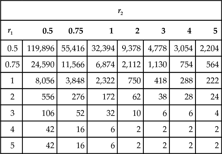
Clearly, the recursive schema theorem presented in this paper will need to be strengthened if we want to use it to size the population in practical applications. However, the procedure indicated in this section demonstrates that in principle this is a viable approach and that useful insights can be obtained already. For example, it is interesting to notice that the population sizes in the table depend significantly more on the order-1/generation-1 building-block fitness ratio r1 than on the order-2/generation-2 building-block fitness ratio r2. This seems to suggest that problems with deceptive attractors for low-order buildingblocks may be harder to solve for a GA than problems where deception is present when higher-order building-blocks are assembled. This conjecture will be checked in future work. In the future it would also be very interesting to compare the population sizing equations derived from this approach with those obtained by others (e.g. see [Goldberg et al., 1992]).
9 CONCLUSIONS AND FUTURE WORK
In this paper we have used a form of schema theorem in which expectations are not present in an unusual way, i.e. to predict the past from the future. This has allowed the derivation of a recursive version of the schema theorem which is applicable to the case of finite populations. This schema theorem allows one to find under which conditions on the initial generation the GA will converge to a solution in constant time. As an example, in the paper we have shown how such conditions can be derived for a generic 4-bit problem.
All the results in this paper are based on the assumption that the fitness of the building blocks involved in the process of finding a solution and the population fitness are known at each generation. Therefore, our results do not represent a full schema-theorem-based proof of convergence for GAs. In future research we intend to explore the possibility of getting rid of schema and population fitnesses by replacing them with appropriate bounds based on the “true” characteristics of the schemata involved such as their static fitness. As indicated in Section 5, several approaches to tackle this problem are possible. If this step is successful, it will allow' to identify rigorous strategies to size the population and therefore to calculate the computational effort required to solve a given problem using a GA. This in turn will open the way to a precise definition of “GA-friendly” (“GA- easy”) fitness functions. Such functions would simply be those for which the number of fitness evaluations necessary to find a solution with say 99% probability in multiple runs is smaller (much smaller) than 99% of the effort required by exhaustive search or random search without resampling.
Since the results in this paper are based on Chebychev inequality and Bonferroni bound, they are quite conservative. As a result they tend to considerably overestimate the population size necessary to solve a problem with a known level of performance. This does not mean that they will be useless in predicting on which functions a GA can do well. It simply means that they will over-restrict the set of GA-friendly functions. A lot can be done to improve the tightness of the lower bounds obtained in the paper. When less conservative results became available, more functions could be included in the GA-friendly set.
Not many people nowadays use fixed-size binary GAs with one-point crossover in practical applications. So, the theory presented in this paper, as often happens to all theory, could be thought as being ten or twenty years or so behind practice. However, there is really a considerable scope for extension to more recent operators and representations. For example, by using the crossover-mask-based approach presented in [Altenberg, 1995][Section 3 and Appendix] one could write an equation similar to Equation 2 valid for any type of homologous crossover on binary strings. The theory presented in this paper could then be extended for many crossover operators of practical interest. Also, in the exact schema theorem presented in [Stephens and Waelbroeck, 1997, Stephens and Waelbroeck, 1999] point mutation was present. So, it seems possible to extend the results presented in this paper to the case of point mutation (either alone or with some form of crossover). Finally, Stephens and Waelbroeck’s theory has been recently generalised in [Poli, 2000b, Poli, 2000a] where an exact expression of (H,t) for genetic programming with one-point crossover was reported. This is valid for variable-length and non-binary GAs as well as GP and standard GAs. As a result, it seems possible to extend the results presented in this paper to such representations and operators, too. So, although in its current form the theory presented in this paper is somehow behind practice, it is arguable that it might not remain so for long.
Despite their current limitations, we believe that the results reported in this paper are important because, unlike previous results, they make explicit the relation between population size, schema fitness and probability of convergence over multiple generations. These and other recent results show that schema theories axe potentially very useful in analysing and designing GAs and that the scepticism with which they are dismissed in the evolutionary computation community is becoming less and less justifiable.
Acknowledgements
The author wishes to thank the members of the Evolutionary and Emergent Behaviour Intelligence and Computation (EEBIC) group at Birmingham, Bill Spears, Ken De Jong and Jonathan Rowe for useful comments and discussion. The reviewers of this paper are also thanked warmly for their thorough analysis and helpful comments. Finally, many thanks to Günter Rudolf for pointing out to us the existence of the Chernoff-Hoeffding bounds.