2

Setting Up the Document Store with MongoDB

In this chapter, we are going to address some of the main features of MongoDB, building upon what was mentioned in the introductory chapter, and then we will dive into a practical introduction through several simple yet illustrative examples. After reviewing the process of installation on a local machine, using Windows or Ubuntu (which is probably the most popular Linux distribution today), and creating an online account on Atlas, we will be covering the basic commands of the MongoDB querying framework that enable us to start as quickly as possible. We will walk you through the essential commands (methods) that will enable you to insert, manage, query, update, and wrangle your data. The aim of this chapter is not to make you a MongoDB expert or even a proficient user, but just to help you see how easy it can be to set up a system—be it on your local machine or on the cloud—and perform the operations that might arise in a fast-paced web development process.

In this chapter, we will cover the following topics:

• The structure of a MongoDB database
• Installing MongoDB and friends
• MongoDB querying and CRUD operations
• Aggregation framework

By the end of this chapter, you will be able to set up a MongoDB database in a local or online environment, and you will know the basics of data modeling with the most popular NoSQL database. Topics such as querying (through MongoDB methods and aggregation) are best learned through playing around with data. In this chapter, we have provided a simple yet interesting real-life dataset that will be your starting point. Finally, this chapter should enable you to import your own data and apply the principles from the following pages, building upon them and coming up with your own queries, aggregations, and data insights.

Technical requirements

MongoDB’s latest version (version 5) requires Windows 10 64-bit or Windows Server 2019 or later. When it comes to Linux, the last three versions of Ubuntu (Debian) are supported. Any decent PC or laptop with at least 8 GB of RAM and a CPU not more than 5 years old should be more than enough to get you started. However, for full-stack development—which means having a couple of processes running simultaneously, compiling the frontend, maybe some CSS processor, having an editor (we will use VS Code), and a browser with a dozen tabs open—if possible, we would recommend 16 GB of RAM and a big screen (protect your eyes because unfortunately, they are not upgradeable!).

The supporting files for this chapter can be found at the following link: https://github.com/PacktPublishing/Modern-Web-Development-with-the-FARM-Stack.

The structure of a MongoDB database

MongoDB is arguably the most used NoSQL database today – its power, ease of use, and versatility make it an excellent choice for large and small projects; its scalability and performance enable us to be certain that at least the data layer of our app has a very solid foundation.

In the following sections, we will take a deeper dive into the basic units of MongoDB: the document, the collection, and the database. Since this book is taking a bottom-up approach, we would like to start from the very bottom and present an overview of the simplest data structures available in MongoDB and then take it up from there into documents, collections, and so on.

Documents

We have repeated numerous times that MongoDB is a document-oriented database, so let’s take a look at what that actually means. If you are familiar with relational database tables (with columns and rows), you know that one unit of information is contained in a row, and we might say that the columns describe that data.

In MongoDB, we can make a rough analogy with the relational database row, but, since we do not have to adhere to a fixed set of columns, the model is much more flexible. In fact, it is as flexible as you want it to be, but you might not want to take things too far in that direction if you want to achieve some real functionality. This flexible document really is just an ordered set of keys and corresponding values. This structure, as we will explore later, corresponds with data structures in every programming language; in Python, we will see that this structure is a dictionary and lends itself perfectly to the flow of data of a web app or a desktop application.

The rules for creating documents are pretty simple: the key must be a string, a UTF-8 character with a few exceptions, and the document cannot contain multiple keys. We also have to keep in mind that MongoDB is case sensitive. Let’s take a look at the following relatively simple valid MongoDB document, similar to the ones that we will be using throughout the chapter:

{
      {"_id":{"$oid":"62231e0a286b06fd01be579e"},
      "brand":"Hyundai",
      "make":"ix35",
      "year":2012,
     "price":9000,
     "km":143500
}

Apart from the first field, denoted by _id, which is the unique ID of the document, all of the other fields correspond to simple JavaScript Object Notation (JSON) fields—brand and make are strings (Hyundai, i35), whereas year, price and km (denoting the year of production, the price of the vehicle in euros, and the numbers of kilometers on the meter) are numbers (integers, to be precise).

So, what data types can we use in our documents? One of the first important decisions when designing any type of application is the choice of data types—we really do not want to use the wrong tools for the job at hand. Let’s look at the most important data types in the following sections.

Strings

Strings are probably the most basic and universal data type in MongoDB, and they are used to represent all text fields in a document. Bear in mind that text fields do not have to represent only strictly textual values; in our case, in the application that we will be building, most text fields will, in fact, denote a categorical variable, such as the brand of the car or the fact that the car has a manual or automatic transmission. This fact will come in handy if you are designing a data science application that has categorical or ordinal variables. As in JSON, text fields are wrapped in quotes. JSON files follow a dictionary-like structure with a string, numbers, arrays, and Booleans of key-value pairs. An example of a string variable called name encoded in JSON would be the following:

"name":"Marko"

Text fields can be indexed in order to speed up searching and they are searchable with standard regular expressions, which makes them a powerful tool able to process even massive amounts of text.

Numbers

MongoDB supports different types of numbers:

• int: 32-bit signed integers
• decimal: 128-bit floating point
• long: 64-bit unsigned integer
• double: 64-bit floating point

Every MongoDB driver takes care of transforming data types according to the programming language that is used to interface, so we shouldn’t worry about conversions except in particular cases that will not be covered here.

Booleans

This is the standard Boolean true or false value; they are written without quotes since we do not want them to be interpreted as strings.

Objects or embedded documents

This is where the magic happens. Object fields in MongoDB represent nested or embedded documents and their values are other valid JSON documents. These embedded documents can have other embedded documents inside, and this seemingly simple capability allows for complex data modeling. An example would be if we wanted to embed the salesman responsible for a particular car, added in bold in the following example:

{
       {"_id":{"$oid":"62231e0a286b06fd01be579e"},
       "brand":"Hyundai",
       "make":"ix35",
       "year":2012,
       "price":9000,
       "km":143500,
       "salesman":{
             "name":"Marko",
             {"_id":{"$oid":"62231e0a286b87fd01be579e"},
             "active":true
                  }
}

Arrays

Arrays can contain zero or more values in a list-like structure. The elements of the array can be any MongoDB data type including other documents. They are zero-based and particularly suited for making embedded relationships – we could, for instance, store all of the post comments inside the blog post document itself, along with a timestamp and the user that made the comment. In our example, a document representing a car could contain a list of salesmen responsible for that vehicle, a list of customer requests for additional information regarding the car, and so on. Arrays can benefit from the standard JavaScript array methods for fast editing, pushing, and others.

ObjectIds

Every document in MongoDB has a unique 12-byte ID that is used to identify it, even across different machines, and serves as a primary key. This field is autogenerated by MongoDB every time we insert a new document, but it can also be provided manually – something that we will not do. These ObjectIds are extensively used as keys for traditional relationships – for instance, every salesperson in our application could have a list of ObjectIds, each corresponding to a car that the person is trying to sell. ObjectIds are automatically indexed.

Dates

Though JSON does not support date types and stores them as plain strings, MongoDB’s BSON format supports date types explicitly. They represent the 64-bit number of milliseconds since the Unix epoch (January 1, 1970). All dates are stored in UTC and have no time zone associated.

Binary data

Binary data fields can store arbitrary binary data and are the only way to save non-UTF-8 strings to a database. These fields can be used in conjunction with MongoDB’s GridFS filesystem to store images, for example. Although, there are better and more cost-effective solutions for that, as we will see.

Other data types worth mentioning are null – which can represent a null value or a nonexistent field, and we can store even JavaScript functions.

When it comes to nesting documents within documents, MongoDB supports 100 levels of nesting, which is a limit you really shouldn’t be testing in your designs, at least in the beginning.

Documents in MongoDB are the basic unit of data and as such, they should be modeled carefully when trying to use the database-specific nature to our advantage. Documents should be as self-contained as possible and MongoDB, in fact, encourages a good amount of data denormalization. As MongoDB was built with the purpose of providing developers with a flexible data structure that should be able to fit the processes of data flow in a web application as easily as possible, you should think in terms of objects and not tables, rows, and columns.

If a certain page needs to perform several different queries in order to get all the data needed for the page and then perform some combine operation, your application is bound to slow down. On the other hand, if your page greedily returns a bunch of data in a single query and the code then needs to go over this result set in order to filter the data that is actually needed, memory consumption will likely rise, and this can lead to a potential problem and slow operations. So, like almost everywhere, there is a sweet spot; a locally optimal solution, if you will.

In this book, we will be using a simple example with automobiles for sale and the documents representing the unit (a car, really) are going to be rather straightforward.

We can think of a scenario where users can post comments or reviews on these cars and the SQL-ish way to do it would be to create a many-to-many relationship; a car can have multiple user comments and a user can leave comments or ratings on multiple cars. To retrieve all of the comments for a particular car, we would then have to perform a join by using that car’s primary key, entering the relationship table, and finding all of the comment IDs. Finally, we would use these comment IDs to filter the comments from the table that stores all of the comments, find their IDs, authors, the actual comments, ratings, and so on.

In MongoDB, we can simply store the comments in an array of BSON objects embedded in the car document. As the user clicks on a particular car page, MongoDB performs one single find query and fetches the car data and all of the associated comments, ready to be displayed. Of course, if we want to make a user profile page and display all of the data and the comments and reviews made by the user, we wouldn’t want to have to scan through all of the cars in the database and check if there are comments. In this case, it would probably be wise to have a separate collection that would store only users, their profiles, and the comments (storage is cheap!). Data modeling is the process of defining how our data will be stored and what relationships and types of relationships should exist between different documents in our data.

Now that we have an idea of what type of fields are available in MongoDB and how we might want to map our business logic to a (flexible) schema, it is time to introduce collections – groups of documents and a counterpart to a table in the SQL world.

Collections and databases

With the notion of the schema flexibility already repeated several times, you might be asking yourself if multiple collections are even necessary? Indeed, if we can store any kind of heterogeneous documents in a single collection (and MongoDB says we can), why bother with separate collections? There are several reasons as follows:

• Different kinds (structures) of documents in a single collection make development very difficult. We could add fields denoting different kinds of documents, but this just brings overhead and performance issues. Besides, every application, whether web-based or not, needs to have some structure.
• It is much faster (by orders of magnitude) than querying for the document type.
• Data locality: Grouping documents of the same type in a collection will require less disk seek time, and considering that indexing is defined by collection, the querying is much more efficient.

Although a single instance of MongoDB can host several databases at once, it is considered good practice to keep all of the document collections used in an application inside a single database. When we install MongoDB, there will be three databases created and their names cannot be used for our application database: admin, local, and config. They are built-in databases that shouldn’t be replaced, so avoid accidentally naming your database the same way.

After reviewing the basic fields, units, and structures that we are able to use in MongoDB, it is time to learn how to set up a MongoDB database server on our computer and how to create an online account on MongoDB.com. The local setup is excellent for quick prototyping that doesn’t even require an internet connection (though in 2022 that shouldn’t be a problem) and the online database-as-a-service Atlas provides several benefits.

First, it is easy to set up, and, as we will see, you can get up and running literally in minutes with a generous free tier database ready for work. Atlas takes away much of the manual setup and guarantees availability. Other benefits include the involvement of the MongoDB team (which tries to implement best practices), high security by default with access control, firewalls and granular access control, automated backups (depending on the tier), and the possibility to be productive right away.

Installing MongoDB and friends

The MongoDB ecosystem is composed of different pieces of software, and I remember that when I was starting to play with it, there was some confusion. It is, in fact, quite straightforward as we will see. Let’s examine the following various components that we will be installing or using in the following part:

• MongoDB Community Edition – a free full-fledged version of MongoDB that runs on all major operating systems (Linux, Windows, or macOS) and it is what we are going to use to play around with data locally.
• MongoDB Compass – a graphical user interface (GUI) for managing, querying, aggregating, and analyzing MongoDB data in a visual environment. Compass is a mature and useful tool that we’ll be using throughout our initial querying and aggregation explorations.
• MongoDB Atlas – the database-as-a-service solution from MongoDB. To be honest, this is one of the main reasons MongoDB is a huge part of the FARM stack. It is relatively easy to set up and it relieves us from manually administering the database.
• MongoDB Shell – a command-line shell that we can use not only to perform simple Create, Read, Update, Delete (CRUD) operations on our database, but also to perform administrative tasks such as creating and deleting databases, starting and stopping services, and similar jobs.
• MongoDB Database Tools – several command-line utilities that enable administrators and developers to export or import data to and from a database, provide diagnostics, or enable manipulation of files stored in MongoDB’s GridFS system.

The MongoDB ecosystem is constantly evolving, and it is quite possible that when you read these pages, the latest version numbers will be higher or some utility might have changed its name. MongoDB recently released a product called Realm, which is a real-time development platform useful for building mobile apps or Internet of Things (IoT) applications, for instance. We will not cover all of the steps necessary to install all the required software as we do not find a huge stack of screenshots particularly inspiring. We will instead focus on the overall procedure and try to pinpoint the key steps that are necessary in order to have a fully functional installation.

Installing MongoDB and Compass on Windows

We will be installing the latest version of MongoDB Community Edition, which at the time of writing is 5.0.6. The minimum requirements listed on the website for the Windows edition are Windows 10 or later, 64-bit editions, or Windows Server 2019. It is important to note that MongoDB supports only 64-bit versions of these platforms. To install MongoDB and Compass, you can refer to the following steps, although we strongly advise you to look at the instructions on the MongoDB website as well, as they might slightly change:

1. To download the installer, head over to the download page at https://www.mongodb.com/try/download/community, select the Windows version, and click on Download as follows:

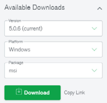
Figure 2.1 – Selecting the latest Windows 64-bit installer from the MongoDB download page

2. When the file is downloaded, locate it on your computer and execute it. If a security prompt asks Open Executable File, select Yes and proceed to the MongoDB setup wizard. The wizard will open the following page:

Figure 2.2 – Starting the MongoDB installer

3. Read the license agreement, select the checkbox, and then click on Next.
4. This is an important screen. When asked which type of setup to choose, select Complete, as follows:

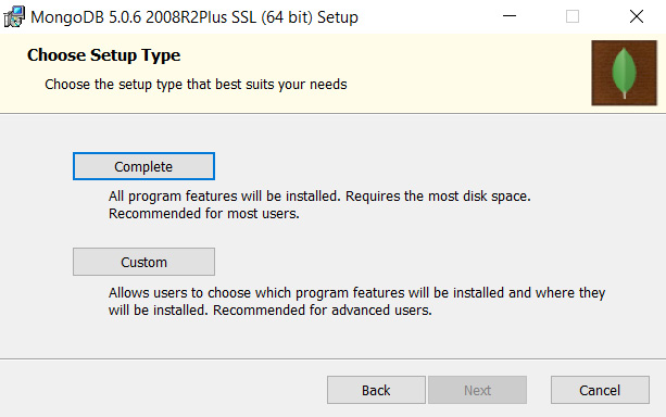
Figure 2.3 – Selecting the Complete installation – click Complete, then Next

5. Another rather important screen follows. The following screen allows us to select whether we want MongoDB to run as a Windows network service (we do) and we can select the data and log directories. We will leave the default values as follows:

Figure 2.4 – The MongoDB service customization screen with the desired (default) values

Figure 2.4 shows that we want to select Install MongoDB—the MongoDB daemon—as a Windows service, which basically means that we will not have to start it manually. The rest of the settings are left as default as well as Data Directory and Log Directory.

6. Another screen will ask you if you want to install Compass, MongoDB’s GUI tool for database management. Please check the checkbox and proceed to install it.
7. Finally, the User Account Control (UAC) Windows warning screen will pop up, and you should select Yes.
8. At this point, we should be able to test whether MongoDB is running (as a service), so enter the following command in the command prompt of your choice (we like to use cmder, available at https://cmder.app) and type the following:

   mongo

9. You should see various notifications and a tiny prompt denoted with >. Try typing the following:

   show dbs

If you see the automatically generated tables admin, config, and locals, you should be good to go.

After installing MongoDB, we can navigate to the default Windows directory that hosts our database files as well as the executable files, as follows:

C:Program FilesMongoDBServer5.0

Let’s check the installation of Compass. We should be able to find it in our start menu under MongoDBCompass (all words attached). It should look like the following:

Figure 2.5 – The initial screen of MongoDB Compass

If we just click the green Connect button, without pasting or typing in any connection string, Compass will connect to the local MongoDB service and we should be able to see all of the databases that we saw when we used the command line with MongoDB: admin, db, and local.

The last local installation that we can and should execute is for a group of utilities called MongoDB Database Tools. You should just head over to https://www.mongodb.com/try/download/database-tools and select the latest version (at the time of writing, it is 100.5.2). The actual download page contains all of the MongoDB-related files and looks like the following:

Figure 2.6 – The MongoDB downloads page

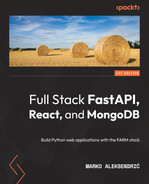
Once you have scrolled to the MongoDB Database Tools tab, you will be presented with a small box on the right – titled Available Downloads. You should choose the latest version, check your platform (in our case it is Windows x86_64) and the .msi Windows package installer, as follows:

Figure 2.7 – The MongoDB Database Tools download page

Be careful to select the .msi package and run the installer using the standard procedure (accept the agreement, confirm the UAC popup, and so on).

The only modification that you should do, although it is not mandatory, is to select the bin directory in the previously installed MongoDB folder. This will facilitate the use of the utilities, although we will mostly use Compass to start playing with some data.

Now we will go through the process of installing MongoDB on a standard Linux distribution.

Installing MongoDB and Compass on Linux – Ubuntu

Linux offers numerous benefits for the development and management of local servers, but most importantly, should you decide that the database-as-a-service of MongoDB isn’t what you want to use anymore, you will probably be going to work on a Linux-based server.

In this book, we will go over the installation process on Ubuntu version 20.4 LTS (Focal), while the MongoDB version supports the last three long-term support (LTS) versions on x86_64 architecture (Focal, Bionic, and Xenial). As in the earlier paragraph for Windows 10, we will list the necessary steps here, but you should always check the MongoDB Ubuntu installation page for last-minute changes. The process, however, shouldn’t change.

The following actions are to be performed in a Bash shell. We are going to download the public key that will allow us to install MongoDB, then we will create a list file and reload the package manager. Similar steps are required for other Linux distributions, so be sure to check them on your distribution of choice’s website. Finally, we will perform the actual installation of MongoDB through the package manager and start the service.

It is always preferable to skip the packages provided by the Linux distribution as they are often not updated to the latest version. Perform the following steps to install MongoDB on Ubuntu:

1. You should import the public key used by the package manager as follows:

   wget -qO - https://www.mongodb.org/static/pgp/server-5.0.asc | sudo apt-key add -

2. After the preceding step has finished installing, you have to create a list file for MongoDB as follows:

   echo "deb [ arch=amd64,arm64 ] https://repo.mongodb.org/apt/ubuntu focal/mongodb-org/5.0 multiverse" | sudo tee /etc/apt/sources.list.d/mongodb-org-5.0.list

3. Reload the package manager as follows:

   sudo apt-get update

4. Finally, install MongoDB as follows:

   sudo apt-get install -y mongodb-org

If you follow these instructions and install MongoDB through the package manager, the /var/lib/mongodb data directory and the /var/log/mongodb log directory will be created during the installation.

5. Start the mongod process using the systemctl process manager as follows:

   sudo systemctl start mongod

   sudo systemctl daemon-reload

6. You should be able to start using the MongoDB shell by typing the following command:

   mongosh

If you have issues with the installation, our first advice would be to visit the MongoDB Linux installation page, but MongoDB isn’t particularly different than any other Linux software when it comes to installation and process management.

Setting up Atlas

MongoDB Atlas—a cloud service by MongoDB—is one of the strongest selling points of MongoDB. As their website puts it:

Database-as-a-Service, is one of the many -as-a-Service web development stages that have been running in the Cloud over the last decade (we also have platforms as a service and others). It just means that all or most part of the database administration and installation work is offloaded to a cloud service in a highly simplified, customizable and optimized procedure. It allows for a fast start, but also offers sensible and often optimal defaults when it comes to security, scalability and performance.

Atlas is a cloud database that manages all the hard work and abstracts the majority of operations such as deployment, management, and diagnostics while running on a provider of our choice (AWS, GCP, or Azure).

We believe that the processes of signing up and setting up a MongoDB Atlas instance are very well documented on the site at https://www.mongodb.com/basics/mongodb-atlas-tutorial.

After setting up the account (we used a Gmail address so we can log in with a Google account – it’s faster), you will be prompted to create a cluster. You will select a Shared Cluster, which is free and you should select the Cloud Provider & Region as close to your physical location as possible in order to minimize latency. After a couple of minutes, you will be greeted by an administration page that can be a bit overwhelming at first. We will just walk you through the important screens. To set up Atlas, perform the following steps:

1. Select a free M0 sandbox, as shown in the following screenshot:

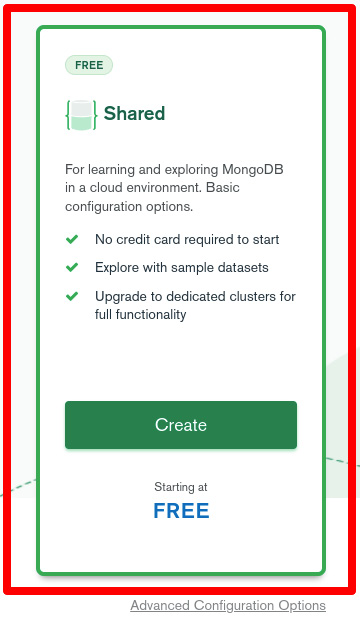
Figure 2.8 – Choose the Shared Cluster on MongoDB Atlas

2. Give your cluster a meaningful name, choose the nearest location in order to minimize latency, and then choose the Shared option as follows:

Figure 2.9 – Atlas deployment options

3. In the menu, create a new database user, choose Password as the authentication method, and create them in the following fields. Later, you can let Atlas autogenerate a super secure password for you, but for now, choose something that will be easy to remember also when creating the connection string for Compass and the later Python connectors.

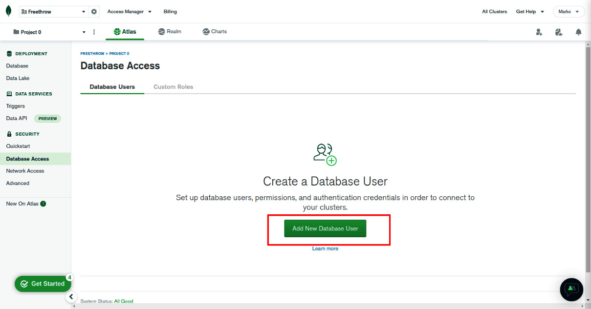
Figure 2.10 – The Database Access screen

4. In this step, select a cloud provider and a region. It is advisable to select the region nearest to your geographical location in order to have the fastest response.

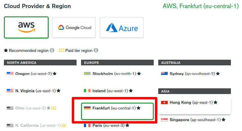
Figure 2.11 – The Cloud Provider & Region screen

5. Finally, you should select the desired cluster tier. Since we want to begin with a free tier, you should select the M0 Sandbox option (shared RAM, 512 MB Storage). Do not worry, you can always change the plan later, and the free tier will be more than sufficient for your initial projects.

Figure 2.12 – Select the M0 Sandbox

6. Then go ahead and add a name for the cluster as shown in the following screenshot:

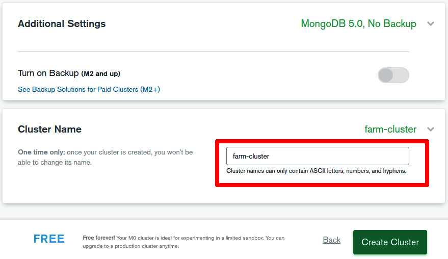
Figure 2.13 – Type a meaningful name for your new cluster

The name isn’t really important at this point, but soon you will have more clusters and it is wise to start naming them properly from the beginning.

7. When you create a new database user, you will be presented with several options for authentication. In this phase, select Password as the authentication method (the first option). In the text boxes that will be underneath it, you should insert your username and password combination. These credentials will be used to access your online database.

Figure 2.14 – Choose a username and password

8. The created user won’t be of much use if you do not give them the privileges to read and write, so check that in the built-in roles dropdown as follows:

Figure 2.15 – Select read and write for the new user

Importing (and exporting) data with Compass

Now, we cannot have even a vague idea of what we can or cannot do with our data if we don’t have any data to begin with. In the GitHub repository of the book, in the chapter2 folder, you will find a comma-separated values (CSV) file called cars_data.csv.

Download the file and save it somewhere handy. To understand the data importing and exporting process, perform the following steps:

1. After you open Compass and click on Connect, without entering a connection string, you will be connected to the local instance of MongoDB that is running as a service on your computer.
2. Click on the Create Database button and insert the database name carsDB and the collection name cars, as follows:

Figure 2.16 – The Create Database screen

3. After this step, a new database should be available in the left-hand menu, called carsDB. Select this database on the left and you will see that we created a collection called cars. In fact, we cannot have a database without collections. There is a big Import Data button in the middle, and you will use it to open a dialog as follows:

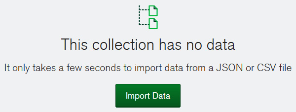
Figure 2.17 – The Import Data button in Compass

4. After hitting the Import Data button, locate the previously downloaded CSV file and you will be presented with the opportunity to tune the types of the individual columns as follows:

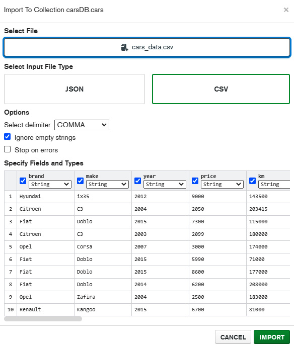
Figure 2.18 – The screen for selecting the file to be imported

This is important, especially because we’re importing initial data and we do not want to have integers or floating numbers being interpreted as strings. The MongoDB drivers, such as Motor and PyMongo, that we will be using are “smart” enough to figure out the appropriate data types; however, when dealing with Compass or similar GUI database tools, it is imperative that you take the time to examine all of the data columns and select the appropriate data types.

This particular file that we imported contains data about 7,323 cars and the default for all the fields is string. We made the following modifications when importing:

• Set the columns year, price, km, kW, cm3, and standard to Number
• Set the imported and registered columns to Boolean

The names of the columns are pretty self-explanatory, but we will examine them more later. Now, once you hit the Import button, you should have a pretty decent collection with a little over 7,000 documents, each having an identical structure that we believe will facilitate the understanding of the operations that we are going to perform later on.

Later, we will see how we can use Compass to run queries and aggregations and export the data in CSV or JSON formats in a pretty similar way to the import that we just did. We suggest that you play around with the interface and experiment a bit. You can always delete the collection and the database, and then redo our data import from the CSV file from the repository.

Now, we will show you how you can connect your Mongo Atlas online database instance to Compass and use the GUI in the exact same way in order to manipulate the online database that we created when we made the Atlas account. Perform the following steps:

1. In order to make Compass connect to a local instance of MongoDB, you do not need to provide any connection string. To connect to an Atlas instance, however, you should head over to the Database Deployments page on Atlas and click on the Connect button as follows:

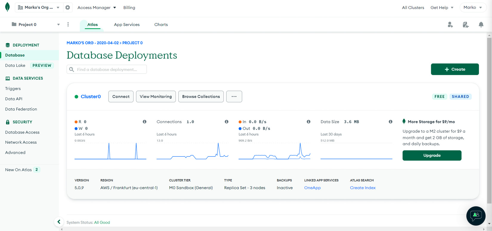
Figure 2.19 – Atlas and Compass connect popup page

2. After clicking on the Connect button, select Connect to Compass, the latest version, and you will be presented with the following screen:

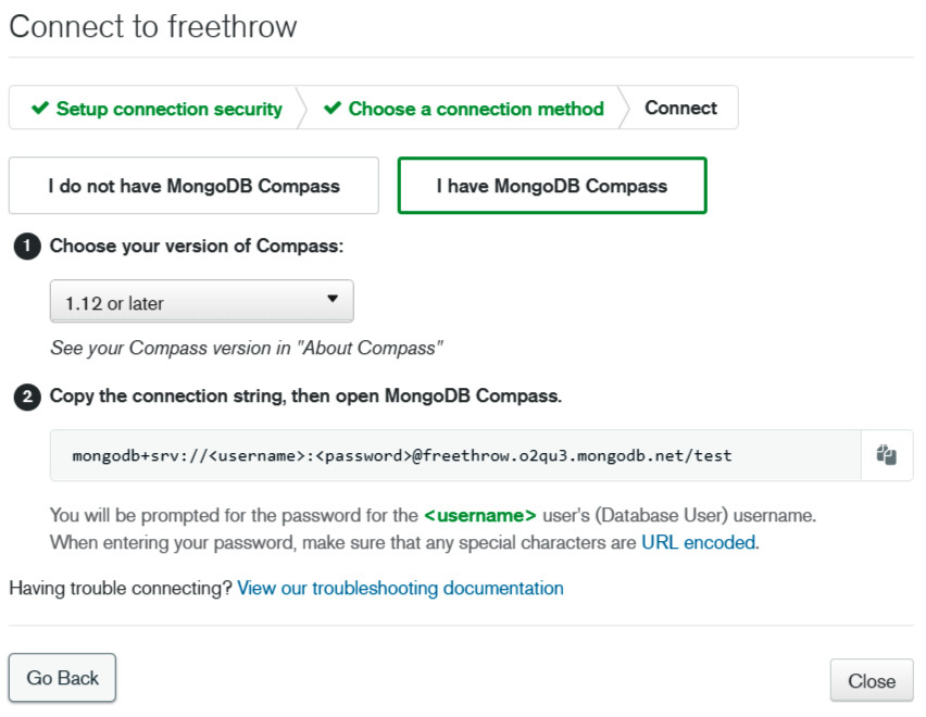
Figure 2.20 – Connection string

3. The connection string, beginning with mongodb+srv://, will be at the bottom of the screen. You should copy it, replace the <username> and <password> with your actual username and password that you previously created, and paste it in the initial screen of Compass in the New Connection field. You should be able to connect!

Phew! We understand that this section was a bit overwhelming, but now you should have a fully functional instance of the world’s most popular NoSQL database on your machine. You have also created an online account and managed to create your very own cluster, ready to take on most data challenges and power your web app. Now it is time to start exploring the bread and butter of MongoDB: querying, creating new documents, updating, and deleting.

MongoDB querying and CRUD operations

After all this setting up, downloading, and installing, it is finally time to see MongoDB in action and try to get what all the fuss is about. In this section, we will show, through some simple examples, the most essential MongoDB commands. Though simple, these methods will enable us, the developers, to take control of our data, create new documents, query documents by using different criteria and conditions, perform simple and more complex aggregations, and output data in various forms. You might say that the real fun begins here!

Although we will be talking to MongoDB through our Python drivers (Motor and PyMongo), we believe that it is better to learn how to write queries directly. We will begin by querying the data that we have imported, as we believe that it is a more realistic scenario than just starting to make up artificial data, then we will go through the process of creating new data – inserting, updating, and so on. Let’s first define our two options for executing MongoDB commands as follows:

• Compass interface
• MongoDB shell

We will now set up both options for working and executing commands on our local database and the cloud database on Atlas as well. Perform the following steps:

1. In a shell session (Command Prompt on Windows or Bash on Linux), run the following command:

   mongo

2. As earlier described when we were testing if the installation succeeded, we are going to be greeted with a minimal prompt: >. Let’s see whether our carsDB database is still present and type the following command:

   show dbs

This command should list all of the available databases: admin, carsDB (our database), config, and local.

3. In order to use our database, let’s type the following code:

   use carsDB

The console will respond with „switched to db carsDB“ and that means that now we can query and work on our database.

4. To see the available collections inside the carsDB, try the following code:

   show collections

You should be able to see our only collection, cars, the one in which we dumped our 7,000+ documents from the downloaded CSV file. Now that we have our database and collection available, we can proceed and explore some querying options.

With Compass, we just have to start the program and click on the Connect button, without pasting the connection string. After that, you should be able to see all of the aforementioned databases in the left-hand menu and you can just select carsDB and then the cars collection, which resembles a folder inside the carsDB database.

Let’s start with some basic querying!

Querying MongoDB

As we mentioned earlier, MongoDB relies on a query language that is based on methods, rather than SQL. This query language has different methods that operate on collections and take parameters as JavaScript objects that define the query. We believe it is much easier to see how querying works, so let’s try out some basic queries. We know we have over 7,000 documents in our carsDB database, and these are real documents that, at a certain point in time a couple of years ago, defined real ads of a used cars sales website. We chose this dataset, or at least a part of it, because we believe that working with real data with some expected query results, and not abstract or artificial data, helps reinforce the acquired notions and makes understanding the underlying processes easier and more thorough.

The most frequent MongoDB query language commands—and the ones that we will be covering—are the following:

• find(): A query for finding and selecting documents matching simple or complex criteria
• insertOne(): Inserts a new document into the collection
• insertMany(): Inserts an array of documents into the collection
• updateOne() and updateMany(): Update one or more documents according to some criteria
• deleteOne() and deleteMany(): Delete documents from the collection

As you can see, the MongoDB query methods closely match the HTTP verbs of a REST API!

We have over 7,000 documents, so let’s take a look at them. To query for all the documents, type in the MongoDB shell the following command:

db.cars.find()

The preceding command will print several documents as follows:

{ "_id" : ObjectId("622c7b636a78b3d3538fb967"), "brand" : "Fiat", "make" : "Doblo", "year" : 2015, "price" : 5700, "km" : 77000, "gearbox" : "M", "doors" : "4/5", "imported" : false, "kW" : 66, "cm3" : 1248, "fuel" : "diesel", "registered" : true, "color" : "WH", "aircon" : "1", "damage" : "0", "car_type" : "PU", "standard" : 5, "drive" : "F" }

{ "_id" : ObjectId("622c7b636a78b3d3538fb968"), "brand" : "Fiat", "make" : "Doblo", "year" : 2015, "price" : 7500, "km" : 210000, "gearbox" : "M", "doors" : "4/5", "imported" : false, "kW" : 66, "cm3" : 1248, "fuel" : "diesel", "registered" : false, "color" : "WH", "aircon" : "2", "damage" : "0", "car_type" : "PU", "standard" : 5, "drive" : "F" }

{ "_id" : ObjectId("622c7b636a78b3d3538fb969"), "brand" : "BMW", "make" : "316", "year" : 2013, "price" : 10800, "km" : 199000, "gearbox" : "M", "doors" : "4/5", "imported" : false, "kW" : 85, "cm3" : 1995, "fuel" : "diesel", "registered" : true, "color" : "VAR", "aircon" : "2", "damage" : "0", "car_type" : "SW", "standard" : 6, "drive" : "B" }

{ "_id" : ObjectId("622c7b636a78b3d3538fb96a"), "brand" : "Citroen", "make" : "C3", "year" : 2010, "price" : 3200, "km" : 142000, "gearbox" : "M", "doors" : "4/5", "imported" : false, "kW" : 50, "cm3" : 1398, "fuel" : "diesel", "registered" : true, "color" : "WH", "aircon" : "2", "damage" : "0", "car_type" : "HB", "standard" : 4, "drive" : "F" }

The console will print the message Type „it“ for more as the console prints out only 20 items at a time. This statement could be interpreted as a classic SELECT * FROM TABLE in the SQL world. Let’s see how we can restrict our query and return only cars made in 2019 (it should be the last available year, as the dataset isn’t really fresh). In the command prompt, issue the following command:

db.cars.find({year:2019})

The results should now contain only documents that satisfy the condition that the year key is equal to 2019. This is one of the keys or CSV fields that, when importing, we have set to the numeric type.

The JavaScript object that we used in the previous query is a filter, and it can have numerous key-value pairs with which we define our query method. MongoDB has many operators that enable us to query fields with more complex conditions than plain equality, and their updated documentation is available on the MongoDB site at https://docs.mongodb.com/manual/reference/operator/query/.

We invite you to visit the page and look around some of the operators as they can give you an idea of how you might be able to structure your queries. We will try combining a couple of them to get a feel for it.

Let’s say we want to find all Ford cars made in 2016 or later and priced at less than 7,000 euros. The following query will do the job:

db.cars.find({year:{'$gt':2015},price:{$lt:7000},brand:'Ford'}).pretty()

Notice that we used three filter conditions: ‘$gt’:2015 means “greater than 2015”, we set the price to be less than 7000, and finally, we fixed the brand to be ‘Ford’. The find() method implies an AND operation, so only documents satisfying all three conditions will be returned. At the end, we added the MongoDB shell function called pretty(), which formats the console output in a bit more readable way. The result should look like the following:

{
        "_id" : ObjectId("622c7b636a78b3d3538fbb72"),
        "brand" : "Ford",
        "make" : "C Max",
        "year" : 2016,
        "price" : 6870,
        "km" : 156383,
        "gearbox" : "M",
        "doors" : "4/5",
        "imported" : true,
        "kW" : 92,
        "cm3" : 1596,
        "fuel" : "petrol",
        "registered" : false,
        "color" : "VAR",
        "aircon" : "2",
        "damage" : "0",
        "car_type" : "VAN",
        "standard" : 5,
        "drive" : "F"
}
{
        "_id" : ObjectId("622c7b646a78b3d3538fce03"),
        "brand" : "Ford",
        "make" : "Fiesta",
        "year" : 2016,
        "price" : 6898,
        "km" : 149950,
        "gearbox" : "M",
        "doors" : "4/5",
        "imported" : false,
        "kW" : 55,
        "cm3" : 1461,
        "fuel" : "diesel",
        "registered" : true,
        "color" : "BL",
        "aircon" : "2",
        "damage" : "0",
        "car_type" : "HB",
        "standard" : 6,
        "drive" : "F"
}

We have seen the find() method in action and we have seen a couple of examples where the find() operator takes a filter JavaScript object in order to define a query. Some of the most used query operators are $gt (greater than), $lt (less than), and $in (providing a list of values), but as we can see from the MongoDB website, there are many more – logical and, or, or nor, geospatial operators for finding the nearest points on a map, and so on. It is time to explore other methods that allow us to perform queries and operations.

findOne() is similar to find() and it takes an optional filter parameter but returns only the first document that satisfies the criteria.

Before we dive into the process of creating or deleting and updating existing documents, we want to mention a very useful method called projection, which allows us to limit and set the fields that will be returned from the query results. The find() (or findOne()) method accepts an additional object that tells MongoDB which fields within the returned document are included or excluded.

Building projections is easy; it is just a JSON object in which the keys are the names of the fields, while the values are 0 if we want to exclude a field from the output, or 1 if we want to include it. The ObjectId is included by default, so if we want to remove it from the output, we have to set it to 0 explicitly. Let’s try it out just once; let’s say that we want the top 5 oldest Ford Fiestas with just the year of production and the kilometers on the meter, so we type the following command:

db.cars.find({brand:'Ford',make:'Fiesta'},{year:1,km:1,_id:0}).sort({'year':1}).limit(5)

We sneaked in two things here, the sort and the limit parts, but we did it on purpose so we can have a glimpse of the MongoDB aggregations (albeit the simplest ones) and to see how intuitive the querying process can be. The projection part, however, is hidden in the second JSON object provided for the find() method. We simply stated that we want the year and the km variable, and then we suppressed _id since it will always be returned by default.

Always reading and sorting the same documents can become a bit boring and quite useless in a real-life environment. In the next section, we will learn how to create and insert new documents into our database. Creating documents will be the entry point to any system that you will be building, so let’s dive in!

Creating new documents

The method for creating new documents in MongoDB is insertOne(). You can try inserting the following fictitious car into our database:

db.cars.insertOne({'brand':'Magic Car','make':'Green Dragon', 'year':1200})

MongoDB will now gladly accept our new car even though it doesn’t look like the earlier imported cars and it will print out the following important message:

{
        "acknowledged" : true,
        "insertedId" : ObjectId("622da66da111a4265fd4f526")
}

The first part means that MongoDB acknowledged the insertion operation, whereas the second property prints out the ObjectId, which is the primary key that MongoDB uses and assigns automatically if not provided manually.

MongoDB, naturally, also supports inserting many documents at once with the insertMany() method. Instead of providing a single document, the method accepts an array of documents.

We could, for example, insert another couple of Magic Cars as follows:

db.cars.insertMany([{brand:'Magic Car',make:'Yellow Dragon',year:1200},{brand:'Magic Car',make:'Red Dragon',legs:4}])

Here we inserted two new highly fictitious cars and the second one has a new property, legs, which does not exist in any other car, just to show off MongoDB’s schema flexibility. The shell acknowledges (reluctantly? We’ll never know) and prints out the ObjectIds of the new documents.

Updating documents

Updating documents in MongoDB is possible through several different methods that are suited for different scenarios that might arise in your business logic.

The updateOne() method updates the first encountered document with the data provided in the fields. For example, let’s update the first Ford Fiesta that we find, add a Salesman field, and set it to Marko as follows:

db.cars.updateOne({make:'Fiesta'},{$set:{'Salesman':'Marko'}})

We can also update existing properties of the document as long as we use the $set operator. Let’s say that we want to reduce the prices of all Ford Fiestas in a linear way (not something you would want to do in real life, though) by 200. You could try it with the following command:

db.cars.updateMany({make:'Fiesta'},{$inc:{price:-200}})

The preceding command updates many documents, namely all cars that satisfy the simple requirement of being a Fiesta (note that if another car producer, like Seat, decided to make a car named Fiesta, we would have to specify the brand as well) and makes use of the $inc operator (increment). Then, we pass the price field and the amount that we wish to increment the value. In our case, that would be minus 200 euros.

Updating documents is an atomic operation – if two or more updates are issued at the same time, the one that reaches the server first will be applied.

MongoDB also provides a replaceOne operator that takes a filter, like our earlier methods, but expects also an entire document that will take the place of the preceding one. It is worth mentioning that there is also a very handy method, within updateOne(), that enables us to check whether the document to be updated exists and then update it, but in the case that no such document exists, the method will create it for us. The syntax is the same as a standard updateOne() method, but with the {"upsert":true} parameter.

Updating single documents should generally involve the use of the document’s ID.

Deleting documents

Deleting documents works in a similar way to the find methods – we provide a filter specifying the documents to be deleted and we can use the delete or the deleteMany method to execute the operation. Let’s delete all of our Magic Car automobiles under the pretext that they are not real, as follows:

db.cars.deleteMany({brand:'Magic Car'})

The shell will acknowledge this operation with a deletedCount variable equal to 3 – the number of deleted documents. The deleteOne method operates in a very similar way.

Finally, we can always drop the entire cars collection with the following command:

db.cars.drop()

Note

Make sure to import the data again from the CSV file if you delete all of the documents or drop the collection since there won’t be any data left to play with!

Cursors

One important thing to note is that the find methods return a cursor and not the actual results. The actual iteration through the cursor will be executed in a particular and customized way through the use of a language driver to obtain the desired results. The cursor enables us to perform some standard database operations on the returned documents, such as limiting the number of results, ordering by one or more keys ascending or descending, skipping records, and so on.

Since we are doing our MongoDB exploration using the shell (maybe you have been experimenting with Compass as well), we should point out that the shell automatically iterates over the cursor and displays the results. However, if we store the cursor in a variable, we can use some JavaScript methods on it and see that it exhibits, in fact, typical cursor behavior.

Let’s create a cursor for the Ford Fiesta cars as follows:

let fiesta_cars = db.cars.find({'make':'Fiesta'})

Now you can play around with the fiesta_cars variable and apply various methods such as next(), hasNext(), and similar cursor operations. The point is that the query is not sent to the server immediately when the shell encounters a find() call, but it waits until we start requesting data. This has several important implications, but it also enables us to apply an array of methods that return the cursor itself, thus enabling the chaining of methods.

Very similarly to jQuery or D3.js if you ever used them, chaining enables a nifty way of applying several operations on a cursor and returning a fine-tuned result set. Let’s see a simple example in action. We want the top 5 cheapest cars made in 2015, as follows:

db.cars.find({year:2015},{brand:1,make:1,year:1,_id:0,price:1}).sort({price:1}).limit(5)

For simplicity, we have added a projection to only return the brand, the model (make), and the year. The following output is what we got:

{ "brand" : "Fiat", "make" : "Panda", "year" : 2015, "price" : 4199 }
{"brand": "Škoda", "make" : "Fabia", "year" : 2015, "price" : 4200 }
{"brand": "Fiat", "make" : "Grande Punto", "year" : 2015, "price" : 4200 }
{"brand": "Fiat", "make" : "Panda", "year" : 2015, "price" : 4300 }
{"brand": "Opel", "make" : "Corsa", "year" : 2015, "price" : 4499 }

Finally, we will take a look at the MongoDB aggregation framework – an extremely useful tool that enables us, the developers, to offload some (or most) of the computing burden of making calculations and aggregations of varying complexity to the MongoDB server and spare our client-side, as well as our (Python-based) backend, some workload. The aggregation framework will prove itself especially valuable when we try to build some analytic charts showcasing prices, years, brands, and models.

Aggregation framework

In the following pages, we will try to provide a brief introduction to the MongoDB aggregation framework, what it is, what benefits it offers, and why it is regarded as one of the strongest selling points of the MongoDB ecosystem.

Centered around the concept of a pipeline (something that you might be familiar with if you have done some analytics or if you have ever connected a few commands in Linux), the aggregation framework is, at its simplest, an alternative way to retrieve sets of documents from a collection; it is similar to the find method that we already used extensively but with the additional benefit of the possibility of data processing in different stages or steps.

With the aggregation pipeline, we basically pull documents from a MongoDB collection and feed them sequentially to various stages of the pipeline where each stage output is fed to the next stage’s input until the final set of documents is returned. Each stage performs some data-processing operations on the currently selected documents, which include modifying documents, so the output documents often have a completely different structure.

Figure 2.21 – Example of an aggregation pipeline

The operations that can be included in the stages are, for example, match, which is used to include only a subset of the entire collection, sorting, grouping, and projections. The MongoDB documentation site is the best place to start if you want to get acquainted with all the possibilities, but we want to start with a couple of simple examples.

The syntax for the aggregation is similar to other methods – we use the aggregate method, which takes a list of stages as a parameter.

Probably the best aggregation, to begin with, would be to mimic the find method. Let’s try to get all the Fiat cars in our collection as follows:

db.cars.aggregate([{$match: {brand:"Fiat"}}])

This is probably the simplest possible aggregation and it consists of just one stage, the $match stage, which tells MongoDB that we only want the Fiats, so the output of the first stage is exactly that.

Let’s say that in the second stage we want to group our Fiat cars by model and then check the average price for every model. The second stage is a bit more complicated, but bear with us, it is not that hard. Run the following lines of code:

db.cars.aggregate([
{$match: {brand:"Fiat"}},
{$group:{_id:{model:"$make"},avgPrice: { $avg: "$price"} }}
])

The second stage uses the $group directive, which tells MongoDB that we want our inputs (in our case, all the Fiat cars available) grouped, and the _id key corresponds to the document key that we want to use as the grouping key. The part {model:“$make“} is a bit counterintuitive, but it just gives MongoDB the following two important pieces of information:

• model: Without quotes or the dollar sign, it is the key that will be used for the grouping, and in our case, it makes sense that it is called model. We can call it any way we want; it is the key that will indicate the field that we are doing the grouping by.
• $make: It is actually required to be one of the fields present in the documents. In our case, it is called make and the dollar sign means that it is a field in the document. Other possibilities would be the year, the gearbox, and really any document field that has a categorical or ordinal meaning. The price wouldn’t make much sense.

The second argument in the group stage is the actual aggregation, as follows:

• avgPrice: This is the chosen name for the quantity that we wish to map. In our case, it makes sense to call it avgPrice, but we can choose this variable’s name as we please.
• $avg: This is one of the available aggregation functions in MongoDB, called accumulator operators, and they include functions such as average, count, sum, maximum, minimum, and so on. In this example, we could have used the minimum function instead of the average function in order to get the cheapest Fiat for every model.
• $price – like $make in the preceding part of the expression, this is a field belonging to the documents and it should be numeric, since calculating the average or the minimum of a string doesn’t make much sense.

The following diagram illustrates this particular aggregation pipeline, with an emphasis on the group stage since we found it the most challenging for newcomers. Once the data is grouped and aggregated the way we wanted it, we can apply other simpler operations, such as sorting, ordering, and limiting.

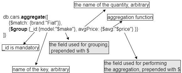
Figure 2.22 – Aggregation with grouping

Pipelines can also include data processing through the project operator – a handy tool for creating entirely new fields, derived from existing document fields, that are then carried into the next stages.

We will provide just another example to showcase the power of project in a pipeline stage. Let’s consider the following aggregation:

db.cars.aggregate([
  {$match:{brand:"Opel"}},
  {$project:{_id:0,price:1,year:1,fullName:
    {$concat:["$make"," ","$brand"]}}},      
   {$group:{_id:{make:"$fullName"},avgPrice:{$avg:            "$price"} }},
  {$sort: {avgPrice: -1}},
  {$limit: 10}
]).pretty()

This might look intimidating at first, but it is mostly composed of elements that we have already seen. There is the $match stage (we select only the Opel cars), and there is sorting by the price in descending order and cutting off at the 10 priciest cars at the end. But the projection in the middle? It is just a way to craft new variables in a stage using existing ones. In fact, the following part of code is a projection:

{$project:{_id:0,price:1,year:1,fullName:
    {$concat:["$make"," ","$brand"]}}},

In the preceding code, which is similar to what we have seen when using the plain old find() method, we use zeroes and ones to show or suppress existing fields in the document, but what about this fullName part? It is just MongoDB’s way of creating new fields by using existing ones. In this case, we use the concatenate function to create a new field, called fullName, that is put together by using the existing make and brand fields. So, the output is the following:

{ "_id" : { "make" : "Movano Opel" }, "avgPrice" : 19999 }

{ "_id" : { "make" : "Crossland X Opel" }, "avgPrice" : 15900 }

{ "_id" : { "make" : "GT Opel" }, "avgPrice" : 15500 }

{ "_id" : { "make" : "Mokka Opel" }, "avgPrice" : 10504.833333333334 }

{ "_id" : { "make" : "Insignia Opel" }, "avgPrice" : 9406.068965517241 }

{ "_id" : { "make" : "Adam Opel" }, "avgPrice" : 7899.75 }

{ "_id" : { "make" : "Antara Opel" }, "avgPrice" : 7304.083333333333 }

{ "_id" : { "make" : "Vivaro Opel" }, "avgPrice" : 6156.5 }

{ "_id" : { "make" : "Signum Opel" }, "avgPrice" : 4000 }

{ "_id" : { "make" : "Astra Opel" }, "avgPrice" : 3858.7214285714285 }

We were able to take a quick look at the MongoDB aggregation framework and we have seen a couple of examples that illustrate the capabilities of the framework. We believe that the syntax and the logic for the grouping stage are the least intuitive parts, whereas the rest is similar to the simple, find-based queries. You are now equipped with a powerful tool that will help you whenever you need to summarize, analyze, or otherwise group and scrutinize your data in an app.

Summary

Trying to condense and reduce the key information about an ecosystem as vast and as feature rich as MongoDB is not an easy task, and we admit that this chapter is heavily influenced by a personal view of what the key takeaways and potential traps are. We learned the basic building blocks that define MongoDB and its structure, and we have seen how to set up a local system as well as an online Atlas account.

You are now able to begin experimenting, importing your own data (in CSV or JSON), and playing with it. You know the basics of creating, updating, and deleting documents and you have a few simple but powerful tools in your developer’s toolbox, such as the find method with its peculiar, yet powerful, filter object syntax, and the aggregation pipelines framework – a strong analytic tool in its own right. You are now able to set up a MongoDB shop anytime, anywhere; start with a free Atlas instance and begin coding, without thinking too much about the infrastructure and with the peace of mind that if, or rather when, the time comes to scale up and accommodate millions of users, your database layer will be ready and won’t let you down.

In the next chapter, we are going to dive into the process of creating APIs – application programming interfaces with FastAPI – an exciting and new Python framework. We will try to provide a minimal, yet complete guide of the main concepts and features that should hopefully convince you that building APIs can be fast, efficient, and fun. Since learning how to build REST APIs with a framework is much easier through practice, we will create a very simple, yet comprehensive API that will allow us to put our freshly created database to good use. We will be able to create new (used) car entries, delete them, update them, and learn how FastAPI solves most typical development problems along the way.