Wave Energy
Abstract
Similar to wind energy, and in contrast to tidal energy, wave energy is a stochastic form of electricity generation. Although modern forecasts make it possible to predict waves with certainty over relatively short timescales (e.g. 24–48 h), any longer-term planning must rely on statistical trends such as seasonal variability. This is one of the challenges of wave energy conversion, another being the extreme nature of the locations where, by their very nature, the wave climate could be suitable for electricity generation. However, wave energy has huge global potential, and its geographical distribution is generally more diverse than tidal energy, which tends to be confined to a relatively low number of ‘hot spots’ such as flow around headlands or through straits. Therefore, there is much global interest, R&D, and investment in wave energy projects and technologies. In this chapter, we investigate the nature of wind waves, through a consideration of linear wave theory, examining fundamental properties of waves such as the dispersion relationship, wave power, and wave transformation in shoaling water. We introduce the various wave energy converter technologies and examine the theory of heaving point absorbers in some detail. Finally, we consider wave resource assessment and characterization, examining timescales of variability, and the theoretical versus technical resource.
Keywords
Wave energy; Linear wave theory; Wave dispersion; Wave power; Wave spectrum; Nonlinear waves; Wave energy converters; Heaving point absorber
Similar to wind energy, and in contrast to tidal energy, wave energy is a stochastic form of electricity generation. Although modern forecasts make it possible to predict waves with certainty over relatively short timescales (e.g. 24–48 h), any longer-term planning must rely on statistical trends such as seasonal variability. This is one of the challenges of wave energy conversion, another being the extreme nature of the locations where, by their very nature, the wave climate could be suitable for electricity generation. However, wave energy has huge global potential, and its geographical distribution is generally more diverse than tidal energy, which tends to be confined to a relatively low number of ‘hot spots’ such as flow around headlands or through straits. Therefore, there is much global interest, R&D, and investment in wave energy projects and technologies.
In this chapter, we investigate the nature of wind waves, through a consideration of linear wave theory, examining fundamental properties of waves such as dispersion wave power, and wave transformation in shoaling water. We introduce the various wave energy converter (WEC) technologies and examine the theory of heaving point absorbers in some detail. Finally, we consider wave resource assessment and characterization, examining timescales of variability, and the theoretical versus technical resource.
5.1 Wave Processes
Looking back at Fig. 1.14, ‘waves’ in the ocean occur over a vast range of scales, from long-period (tidal) waves, with a period of several hours, to capillary waves that have periods of less than 0.1 s. However, the waves that are suitable for electricity generation within the context of ‘wave energy’ are wind waves and swell waves, which generally have periods in the range 2–25 s. Wind waves are generated due to transfer of wind energy and momentum into the wave field. Initially, when a sea surface is calm, small pressure fluctuations associated with turbulence in the airflow above the water surface are sufficient to induce small ripples, or dimples, on the sea surface. Once these ripples have formed, the small slopes provide a mechanism for horizontal winds to act further upon the sea surface, leading to the development of sizeable waves. These locally generated waves are known as ‘wind waves’, and waves that propagate far from their source of generation are known as ‘swell waves’.
There are various properties of ocean waves that are common to almost all waves that occur in the natural environment. Consider a ‘linear’ wave in the space domain that can be represented by a sinusoidal profile (Fig. 5.1). The maximum displacement of the wave from still water level (z = 0) is the wave amplitude, a. The vertical distance between the crest and trough (i.e. 2a) is defined as the wave height, H, and the distance between two successive crests (or troughs) is the wave length, L. Although not shown in Fig. 5.1, a corresponding sketch in the time domain would show that the time between two successive wave crests (or troughs) is the wave period, T. The reciprocal of the wave period (1/T) is the wave frequency, with units of s−1 or Hz.

As all trigonometric functions repeat over the interval 2π, the mathematical description of waves is much simplified if we introduce the concepts of wavenumber (k = 2π/L) and angular frequency (σ = 2π/T). To give the wavenumber physical meaning, k is the number of complete wave cycles that exist in 1 m of linear space. A commonly reported property of waves is the significant wave height (Hs). This is defined as the mean height of the highest one-third of the waves in a record. This approximately corresponds to the wave height that can be estimated visually by a trained observer.
5.1.1 Linear Wave Theory
Waves in the ocean are nonlinear, and do not exactly follow linear wave theory; nevertheless, linear wave theory is very helpful in understanding and assessing more complicated waves such as nonlinear, irregular, and random waves, which will be discussed further later in this chapter. Linear wave theory can also be applied to many engineering and science problems with reasonable accuracy. A detailed derivation of linear wave theory can be found in many standard wave mechanic textbooks. Here, we present the main assumptions, parameters, equations, and wave properties associated with linear wave theory.
The main assumptions of linear wave theory can be summarized as [1]:
- • The fluid is incompressible and inviscid.
- • The flow is irrotational.1
- • The bed is horizontal with a constant depth; the bed is impermeable.
- • The wave amplitude is small.
- • A regular wave with a constant wave period is considered.
- • Coriolis effects are neglected.
- • Waves are long-crested: the hydrodynamic solution is provided for a 2D vertical plane.
- • The pressure at the water surface is constant.
Referring back to Chapter 2, we mentioned that the Euler equations represent an incompressible and inviscid flow as follows:
∇⋅u=0
dudt=∂u∂t+u⋅∇u=−1ρ∇p−gˆk
The Euler equations are the governing equations of an ideal fluid. A particular case of interest is potential flow, in which the flow vorticity is also zero. The other term, which is commonly used in potential flow theory, is irrotational flow (i.e. zero vorticity). Irrotational flow is simply a flow in which the particles do not rotate. It can be shown that the rate of rotation of particles in a flow field is directly proportional to the curl (i.e. ∇×) of velocity
→ω=12∇×u
where →ω![]() is called vorticity (i.e. rotation vector); hence, irrotational flows have zero vorticity. Referring to Eq. (5.2), if we take the curl of this equation, the RHS will become zero, and this leads to
is called vorticity (i.e. rotation vector); hence, irrotational flows have zero vorticity. Referring to Eq. (5.2), if we take the curl of this equation, the RHS will become zero, and this leads to
d(∇×u)dt=d→ωdt=0
In other words, the flow vorticity is constant for ideal flow. Therefore, by assuming that the flow is inviscid and incompressible, we cannot necessarily conclude that the flow is irrotational. Nevertheless, irrotational flow is a special case in this context, where vorticity is not only constant, but it is also zero (i.e. →ω=∇×u=0![]() ). In hydrodynamics and wave mechanics, it is much easier to deal with incompressible, inviscid and irrotational flows, because a scalar potential function can satisfy the governing equations and provide us with the hydrodynamic flow field. This is referred to as potential flow theory. Through some mathematical manipulation, you can easily show that the curl of a gradient of any scalar function is always zero. In other words,
). In hydrodynamics and wave mechanics, it is much easier to deal with incompressible, inviscid and irrotational flows, because a scalar potential function can satisfy the governing equations and provide us with the hydrodynamic flow field. This is referred to as potential flow theory. Through some mathematical manipulation, you can easily show that the curl of a gradient of any scalar function is always zero. In other words,
∇×∇Φ=0and∇×u=0⇒u=∇Φ
where Φ is called the potential function, which as mentioned is a scalar function. In potential flow theory, the flow velocity is the gradient of this potential function. The momentum equation is already satisfied because d→ωdt=d0dt=0![]() . For the continuity equation, we have
. For the continuity equation, we have
∇⋅u=0⇒∇⋅u=∇⋅(∇Φ)=0⇒∇2Φ=0
This is called the Laplace equation, and for a 2D wave field can be expanded as follows:
∇2Φ=∂2Φ∂x2+∂2Φ∂z2=0
In linear wave theory, it is assumed that the flow is inviscid, incompressible, and irrotational; therefore, a potential function, which satisfies the periodic boundary conditions, will be the solution.
Consider a sinusoidal progressive wave (Fig. 5.1). The basic parameters such as wave length (L), wave height (H), still water depth (d), and water surface elevation (η) are presented in this figure. For a progressive wave, it can be shown that the potential function is given by
Φ=H2gσcoshk(d+z)coshkdsin(kx−σt)
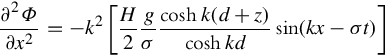
where k is the wave number and σ is the wave angular frequency. Although we skipped the derivation of this equation, let us just show that the above solution satisfies the Laplace equation. Taking the derivatives of the potential function leads to
∂2Φ∂x2=−k2[H2gσcoshk(d+z)coshkdsin(kx−σt)]
∂2Φ∂z2=k2[H2gσcoshk(d+z)coshkdsin(kx−σt)]

⇒∂2Φ∂x2+∂2Φ∂z2=0

Also, the potential function (Eq. 5.8) is periodic. This is because Φ(x,z,t)=Φ(x,z,t+T)=Φ(x,z,t+2πσ)![]() , which is demonstrated as follows
, which is demonstrated as follows
sin(kx−σ[t+2πσ])=sin(kx−σt−2π)=sin(kx−σt)

Using linear wave theory, all of the hydrodynamic variables, including velocity, pressure, water surface elevation, and wave celerity, can be derived from the potential function and implementation of the boundary conditions. Table 5.1 summarizes the wave properties based on linear wave theory.
Table 5.1
| Wave Property | Equation |
|---|---|
| Velocity potential | Φ=H2gσcoshk(d+z)coshkdsin(kx−σt) |
| Wave celerity | C=LT=σk |
| Horizontal component of velocity | u=∂Φ∂x=H2gkσcoshk(d+z)coshkdcos(kx−σt) |
| Vertical component of velocity | v=∂Φ∂z=H2gkσsinhk(d+z)coshkdsin(kx−σt) |
| Wave surface displacement | η=H2cos(kx−σt) |
| Pressure (hydrostatic + dynamic) | p=−ρgz+ρgcoshk(d+z)coshkd(H2cos(kx−σt))=po+pD |
| Horizontal acceleration | ax=∂u∂t=gkH2coshk(d+z)coshkdsin(kx−σt) |
| Vertical acceleration | az=∂w∂t=−gkH2sinhk(d+z)coshkdcos(kx−σt) |
| Dispersion | C2=gktanhkd |
5.1.2 Relationship Between Wave Celerity, Wave Number, and Water Depth: The Dispersion Equation
Wave celerity is dependent on water depth and wave length, and important wave processes such as wave refraction can be explained by the dependence of wave celerity on depth (Section 5.2.2). The relation of wave celerity and water depth can be derived by implementing the (kinematic) free surface boundary condition, which implies that the vertical speed of water particles at the water surface is equal to the speed of the free surface (i.e. v=dηdt=∂η∂t+u∂η∂t![]() at the water surface). Assuming a small amplitude wave, it results in
at the water surface). Assuming a small amplitude wave, it results in
C2=gktanhkd⇒σ2=gktanhkd
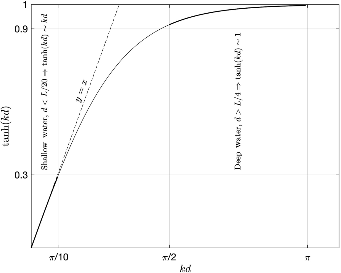
which is called the dispersion equation, because waves of different celerities will be dispersed according to their wave length. Looking at Fig. 5.2, the hyperbolic tangent function (tanhkd![]() ) in the dispersion equation approaches 1 for large depth values (deep water waves) and kd for small values of depth (shallow water waves). Therefore,
) in the dispersion equation approaches 1 for large depth values (deep water waves) and kd for small values of depth (shallow water waves). Therefore,
C2=gk⇒σ2=gk:deep water waves
C2=gk(kd)⇒C2=gd:shallow water waves
Note that the shallow water wave approximation is nondispersive, because it does not relate the wave celerity to wave length.
5.1.3 Wave Energy and Wave Power
Assume that a regular wave, with a wave period T and wave height H, is propagating in constant water depth d. Power (the rate of energy conversion) is the product of velocity and force. In linear wave theory, the force is generated by pressure (i.e. F = pA). Referring to Table 5.1, pressure depends on z. Therefore, wave power can be evaluated by multiplying the pressure and velocity and integrating over depth; the wave power, or more specifically the average energy flux per unit width over a wave period, is given by
P=∫T0∫η−dpDudzdt=18ρgH2C{12(1+2khsinh2kh)}=ECg=cst

Cg=C{12(1+2khsinh2kh)}
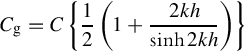
where pD is the dynamic pressure and u is the horizontal velocity given in Table 5.1. Note that wave power is conserved in linear wave theory (i.e. the RHS of Eq. (5.16) is constant).
In the above formulation, E=18ρgH2![]() is the total mechanical energy (i.e. potential and kinetic) of waves per unit surface area averaged over a wave period. In other words, wave power is simply the product of wave energy and wave group velocity. The group velocity Cg (which is dependent on the wave celerity C, wave number k, and water depth) is the speed of wave energy propagation. Referring to the dispersion equation, it is also defined as [1]
is the total mechanical energy (i.e. potential and kinetic) of waves per unit surface area averaged over a wave period. In other words, wave power is simply the product of wave energy and wave group velocity. The group velocity Cg (which is dependent on the wave celerity C, wave number k, and water depth) is the speed of wave energy propagation. Referring to the dispersion equation, it is also defined as [1]
Cg=∂σ∂k=∂∂k√gktanh(kh)
In realistic ocean environments, ocean currents, which are generated by tides, wind, or temperature, affect the propagation of wave energy. Tidal waves and wind waves can be regarded as long and short waves, which interact in various ways. The Doppler shift (which is explained in Chapter 7) is an example where the frequency of waves is influenced by currents:
ω=σ+ku→∂ω∂k=∂σ∂k+u
where σ is the relative wave frequency (observed in a coordinate system moving with the same velocity as the ambient current), ω is the absolute wave frequency (observed in a fixed frame), and u is the ambient current velocity. The wave energy flux when we have ambient currents becomes
C*g=Cg+u→EC*g=ECg+uE≠cst
where Cg* is the group velocity in the presence of ambient currents, ECg is the wave energy transport by the group velocity, and uE is the wave energy transport by tidal currents. When waves propagate in the presence of currents, the wave energy flux is no longer conserved. This happens due to the exchange of energy between wave and current fields. To avoid this issue, wave models apply the conservation of the wave action (E/σ), rather than conservation of wave energy in their formulations (e.g. [2]). Nevertheless, the total energy flux due to waves and currents is conserved. Therefore, the conservation of energy, in a more general way, can be expressed as follows [3]
[ECg+Eu]+{12ρghu3}+{u(2CgC−12)E}=cst
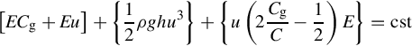
It is clear that when ambient currents are zero, the earlier equations reduce to P = ECg = cst.
5.1.4 Irregular Waves
So far, we have considered a wave that is characterized by a single frequency and direction (i.e. a monochromatic wave). Monochromatic waves can be generated in laboratories (wave tanks), but are rarely seen in the ocean. Waves, which have been generated by wind, are irregular and include many wave frequencies. As ‘wind waves’ travel over long distances, they are dispersed, because the wave celerity/speed is dependent on the frequency. These waves are called ‘swell waves’ and are more similar to regular waves.
Within the range of validity of linear wave theory (see the next section), we can superimpose several monochromatic/sine waves to construct a more realistic irregular wave. Conversely, we can decompose an irregular wave into a number of sinusoidal waves, which have different frequencies. Mathematically speaking, this is the concept of the Fourier series/integral, which is based on the principal that any function can be constructed by combining a set of simple sine waves. This is a powerful method, because we can also find the wave properties, such as pressure, acceleration, and energy, by combining/superimposing the hydrodynamic field of these individual sine waves.
Two main approaches exist to deal with irregular waves: statistical and spectral. In the statistical approach, statistical variables are calculated and used to represent irregular waves. For instance, parameters such as the average wave period, and the root mean square wave height, can be used to represent the wave period, and the wave height, respectively, for a realistic sea state. In this approach, the sea state is represented by a probability distribution function such as Rayleigh, and statistical parameters are derived from that distribution. The spectral method is based on the concept of the Fourier transform and is the basis of spectral wave models, such as SWAN [2], TOMAWAC [4], or STWAVE [5], which are commonly used for wave energy resource characterization. A detailed discussion about irregular waves is beyond the scope of this book and can be found in many other resources (e.g. [1, 6]). Here, basic concepts, with a focus on wave power, are presented.
As mentioned, we can combine several waves with a range of frequencies and phases, to construct an irregular wave, or vice versa. Mathematically speaking, this means
η(t)=∑Ni=1aisin(σit+gi)
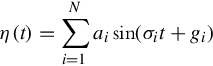
where ai and gi are the amplitude and phase of an individual sine wave, respectively, and η represents the time series of an irregular wave. The total energy of this irregular wave is found by adding up the energy of all sine waves as follows
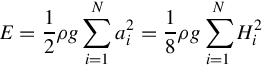
E=12ρg∑Ni=1a2i=18ρg∑Ni=1H2i
Each individual sine wave has a different frequency, and different wave energy, which contributes to the total wave energy. Fig. 5.3 shows an example. An irregular wave has been decomposed into four sine waves, with frequencies of 0.1, 0.2, 0.3, and 0.4 Hz and varying amplitudes. The distribution of the amplitudes of these waves versus frequency is shown in this figure. The plot of the energy of these sine waves (or the square of the amplitude) with respect to the frequency represents the energy spectrum. In other words, the energy spectrum shows how the total energy of an irregular wave is distributed amongst various frequencies. If we use many sine waves to decompose the time series of an irregular wave, the difference between the frequencies of these individual sine waves approaches zero; this will lead to a continuous wave spectrum. A continuous energy density spectrum is defined as
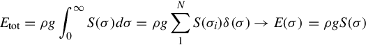
Etot=E(δσ)+E(2δσ)+⋯+E(∞)=∫∞0E(σ)dσ

where E(σ) is called the ‘energy density spectrum’, because it is energy per unit angular frequency (J/rad). Alternatively, the ‘variance density spectrum’ (S(σ); m2/rad) can be used to represent the distribution of energy with respect to frequency. It is defined as,
Etot=ρg∫∞0S(σ)dσ=ρg∑N1S(σi)δ(σ)→E(σ)=ρgS(σ)
Considering Eqs (5.23), (5.25), we can see that the variance density spectrum represents the square of the amplitude of each individual sine wave:
12a2i=S(σi)δσ

The moments of the variance density spectrum are frequently used to compute statistical wave properties. The rth moment (mr) is defined as
mr=∫∞0σrS(σ)dσ

For instance, the significant wave height Hmo, which is the mean of the highest one-third of waves in a record, is given by
Hmo=4√m0
Wave Power for Irregular Waves
Let us start with the total wave energy of a wave spectrum. By definition, the wave energy (in Joules) can be computed as
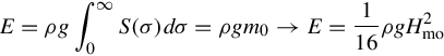
E=ρg∫∞0S(σ)dσ=ρgm0→E=116ρgH2mo
in which we used the following relation
Hmo=4√m0→m0=116H2mo
Because irregular waves can be represented by a wave energy spectrum, we can assume that the total wave power is calculated by adding the wave power of individual waves, which construct the wave spectrum. The wave power of an individual wave with a frequency of σ is given by
ΔP=ρgCg(σ)ΔS(σ)=ρgCgS(σ)Δσ=ρgσk{12(1+2kdsinh2kd)}S(σ)Δσ

Consequently, the total power becomes
P=ρg∫∞0Cg(σ)S(σ)dσ=∫∞0σk{12(1+2kdsinh2kd)}S(σ)dσandσ2=gktanh(kd)

The earlier equation is hard to implement, unless we use spectral wave models or measured data that include the full wave spectrum. Let us formulate the wave power equation for deep waters, in which the dispersion equation is much simpler. As mentioned in Section 5.1.2, in deep waters, tanhkd![]() approaches 1. Therefore, the dispersion equation and the group velocity are given by
approaches 1. Therefore, the dispersion equation and the group velocity are given by
tanhkd≈1→σ=√gk
→Cg=dσdk=g21√gk=g2σ=gT4π

Replacing the group velocity in Eq. (5.32), results in
P=ρg∫∞0Cg(σ)S(σ)dσ=ρg∫∞0g2σS(σ)dσ=12ρg2∫∞0σ−1S(σ)dσ

or
P=12ρg2m−1
For the case of monochromatic waves in deep waters, the wave power becomes
P=CgE=gT4π18ρgH2=ρg232πH2T

If we wanted to use simple wave statistical parameters to compute the wave power (something similar to the previous equation, which only depends on the wave height and the wave period), we can also use the deep water approximation for irregular waves.
Assuming the deep water approximation, the group velocity (which is the speed of propagation of the wave energy) is Cg=gTE4π![]() ; we called the period TE the energy wave period, as it determines the average speed of wave energy propagation. Further, the total wave energy of a spectrum is given by Eq. (5.29) in terms of mo or the significant wave height. Therefore, we can write
; we called the period TE the energy wave period, as it determines the average speed of wave energy propagation. Further, the total wave energy of a spectrum is given by Eq. (5.29) in terms of mo or the significant wave height. Therefore, we can write
P=CgE=gTE4π(ρgm0)=gTE4π(116ρgH2mo)

P=ρg264πH2moTE=ρg232π(Hmo/√2)2TE

which is very similar to Eq. (5.37). In fact, we can use the monochromatic wave equation, if we replace the wave period by the energy wave period, and wave height by Hmo/√2![]() , which is called Hrms or the root-mean-square wave height.
, which is called Hrms or the root-mean-square wave height.
Finally, we can find out how the energy wave period can be calculated based on a wave spectrum. By comparing Eqs (5.36), (5.38),
P=gTE4π(ρgm0)=12ρg2m−1→TE=2πm−1m0
which is equivalent to Tm−10 in spectral models such as SWAN.
In brief, wave power can either be computed using the wave spectrum (i.e. Eq. 5.32) or by using a simplified equation based on the statistical wave parameters (energy/average wave period and significant wave height; Eq. (5.39)). The simplified method is based on the deep water wave approximation, which is generally valid in the vicinity of WECs. The range of water depths where a WEC is installed depends on the device (40 m is a typical depth). Consider a wave with a period of 8 s, propagating in 40 m water depth. The wave length is (from the dispersion equation) L = 2π/k = 99 m, and therefore kd = 2.54 < π; for this wave, tanh(kd)=0.98![]() which is close to 1 and hence, the deep water approximation is valid.
which is close to 1 and hence, the deep water approximation is valid.
5.1.5 Nonlinear Waves
Linear wave theory is the basis of many analytical methods and numerical models, which describe the properties and propagation of regular/irregular waves in the open ocean and coastal regions. Nevertheless, we should be aware of the range of validity of this theory, and wave processes which cannot be explained by this theory. Referring to Section 5.1.1, several assumptions were made to develop linear wave theory, which may not be valid in real-word applications. In particular, in the derivation of linear wave theory, it is assumed that the amplitude of the wave is small compared with the water depth and wave length. Fig. 5.4 shows the range of validity of linear wave theory. As you can see, for deep waters (e.g.dgT2>10−3)![]() and small amplitude waves (e.g.HgT2<10−3)
and small amplitude waves (e.g.HgT2<10−3)![]() , linear wave theory is valid; however, in shallow waters and for large amplitude waves, other wave theories such as Stokes and Cnoidal are more appropriate. Note that in certain depths, or for certain wave steepnesses, the wave is no longer stable and will break. This is discussed further in the following section, and is shown by breaking criteria on this figure (shallow and deep criteria).
, linear wave theory is valid; however, in shallow waters and for large amplitude waves, other wave theories such as Stokes and Cnoidal are more appropriate. Note that in certain depths, or for certain wave steepnesses, the wave is no longer stable and will break. This is discussed further in the following section, and is shown by breaking criteria on this figure (shallow and deep criteria).

Wave Breaking
When the wave height, and consequently wave steepness (i.e. the ratio of wave height to wave length) increase, the water surface profile deviates from a sinusoidal wave shape. The wave eventually breaks if the wave steepness becomes too high.
Miche’s breaking limit criterion, which was proposed in 1944, can approximately predict wave breaking in deep or shallow waters [7]. It can be written as follows,
kHbγtanhkd=1
where Hb is the breaking wave height and γ is a constant parameter. In shallow water, wave breaking occurs due to a decrease in water depth and shoaling (see Section 5.2.1). Looking at Fig. 5.2, in shallow waters, tanhkd≈kd![]() , which results in the following breaking limit criterion:
, which results in the following breaking limit criterion:
kHbγkd=1→Hbd=γ≈0.7−0.8
In deep waters (see Fig. 5.2), tanhkd≈1![]() ; therefore, Miche’s formula leads to the following relation:
; therefore, Miche’s formula leads to the following relation:
kHb/2=γ/2andγ/2≈0.44−0.55
→HbL=γ2π≈0.14−0.17
which is consistent with what we see in Fig. 5.4, and simply indicates that the wave steepness (i.e. kH/2 or H/L depending how it is defined) cannot go beyond a threshold; see other resources for more details about this limit [8].
Nonlinear Dispersion Equation
As we discussed, the linear dispersion equation relates the water depth and the wave frequency to the wave celerity (or wave length). If nonlinear effects are considered, the dispersion equation will also be dependent on the wave height. The nonlinear dispersion equation is given by [9]
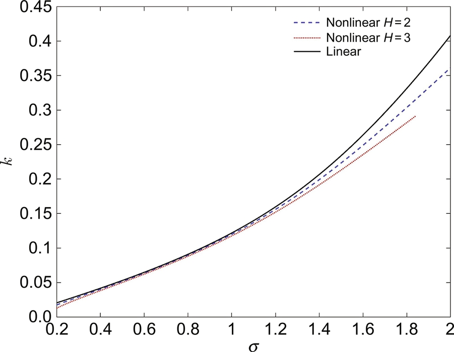
σ2=gktanhkd[1+(kH2)2(8+cosh4kd−2tanh2kd8sinh4kd)]

As can be seen, when kH/2 or the wave steepness is small, the previous equation approaches what we already saw in the linear wave theory (Eq. 5.13). Fig. 5.5 shows the comparison between the linear and nonlinear dispersion equations for two wave heights (2 and 3 m), assuming a water depth of 10 m. You can try to reproduce these plots by solving the linear and nonlinear dispersion equations.
5.2 Wave Transformation Due to Shoaling Water
In general, waves that are generated as a result of a distant storm or localized wind event propagate and ‘disperse’, relatively unhindered, until they encounter shoaling water. At this stage, two processes influence waves: shoaling and refraction.
5.2.1 Wave Shoaling
As water shoals, remembering that waves transport energy in the direction of wave advance, it is important to make use of the principal that wave energy flux per unit surface area, ECg, is constant. This assumes that no energy is dissipated by the wave train, for example, by wave breaking or bottom friction, as it propagates from deep to shallow water. If we apply a subscript ‘0’ to represent deep water values, this implies that
ECg=E0Cg0=constant
Therefore, if we have knowledge of ‘deep water’ wave properties, we can determine the corresponding wave properties in shoaling water.
Consider a horizontally 1D case, in which the wave crests are everywhere parallel to the depth contours (Fig. 5.6). As the waves propagate through water of gradually decreasing depth (shoaling water), their phase speed, and consequently their group velocity, reduces (Eq. 5.13), but their frequency tends to remain constant—in other words, waves do not catch one another up in the same way that they would if they were ‘dispersing’. By way of illustration, for a wave period T = 8 s we can calculate the wave properties shown in Fig. 5.6 and Table 5.2 between ‘deep’ and ‘shallow’ water.
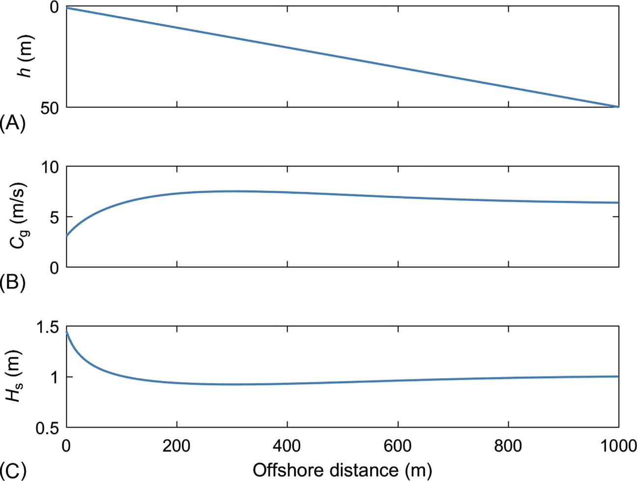
Table 5.2
| Environment | L (m) | C (m/s) | Cg (m/s) |
|---|---|---|---|
| Deep | 100 | 12.5 | 6.2 |
| Shallow | 25 | 3.1 | 3.1 |
![]()
Therefore, a fourfold reduction in wavelength and phase speed is accompanied by a halving of the group velocity. Since E = 1/2ρga2, when Cg is halved, it follows that E is doubled (Eq. 5.46), and so wave amplitude increases by a factor of √2![]() (Fig. 5.6C). This is known as wave shoaling. Note that this illustration is for a 1D case (Fig. 5.6A), but for a more generalized case, another process can complicate wave transformation in shoaling water—refraction.
(Fig. 5.6C). This is known as wave shoaling. Note that this illustration is for a 1D case (Fig. 5.6A), but for a more generalized case, another process can complicate wave transformation in shoaling water—refraction.
5.2.2 Wave Refraction
In the earlier shoaling example, the wave crests were parallel to the depth contours, and the wave propagated normal to the coastline. In most situations, waves propagate obliquely to the depth contours, and are observed to slowly change direction as they approach the coast. This gradual change in wave direction is known as refraction.
Examining Fig. 5.7, which shows wave crests propagating at an oblique angle to the depth contours, there is a variation in water depth experienced along each of the wave crests. Whereas further offshore the wave crest is propagating in relatively deep water, the part of the wave crest closer to the coast is propagating in relatively shallow water. Since wave celerity is related to water depth through the dispersion equation (5.13), this means that the portion of the wave crest in deeper water is travelling faster than the portion of the wave crest that is travelling in shallower water. As a result of this change in phase speed along each wave crest, in a given time interval the crest moves over a larger distance in deeper water than it does in shallower water, and so the waves tend to turn (i.e. refract) towards the depth contours as they propagate.

Variation of ψ (the angle of incidence of the wave orthogonal to the outward normal of the coastline; see Fig. 5.7) is governed by Snell’s law. This is the familiar law from studies of optics and, in the present context, expresses the constancy of wavenumber k in the direction parallel to the shore. In other words, the distance between successive crests measured parallel to the shoreline, L1, remains constant as the waves travel into shallow water (Fig. 5.7). This condition may be written as
ksinψ=k0sinψ0=constant
Based on Eq. (5.47), refraction diagrams can be generated for given offshore wave conditions and maps of bathymetry/topography. However, such analysis is based on the following assumptions [10]:
- • The wave energy between wave rays (orthogonals) remains constant.
- • The direction of wave advance is perpendicular to the wave crest.
- • The speed of the wave of a given period depends only on the water depth at that location.
- • Changes in bathymetry are gradual.
- • Waves are long-crested, constant-period, small-amplitude, and monochromatic.
- • Effects of currents, winds, and reflections from beaches, and underwater topographic features, are considered negligible.
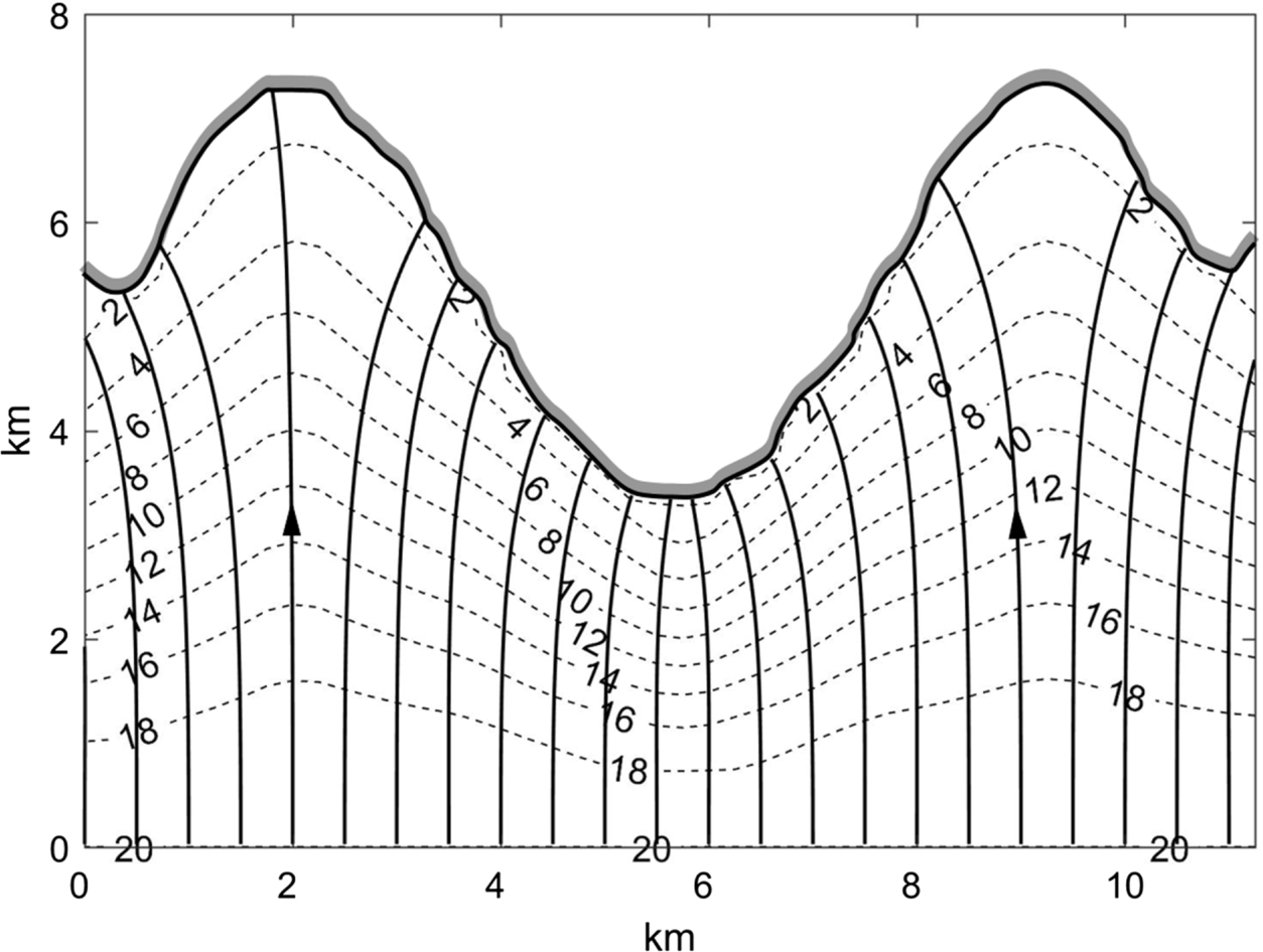
A typical refraction diagram, for a wave of period T = 10 s, is shown for an irregular coastline (a headland and two bays) in Fig. 5.8. The wave orthogonals converge at the headland and diverge in the bays. Because wave energy between the wave orthogonals remains constant (see the earlier assumptions), this implies that the wave height will generally increase at the headland and reduce in the two bays.
As we saw in Eq. (5.46), wave energy flux is a constant, provided no energy is dissipated, for example, by wave breaking or friction. Now, in the more general case, this flux towards the coast is a constant per unit distance parallel to the shoreline
¯ECgcosψ=constant
Therefore, the variation in wave amplitude may be expressed in terms of deep water reference values as follows
a=a0[Cg0Cg]1/2[cosψ0cosψ]1/2
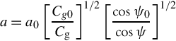
This result shows that, since ψ0 > ψ in general, waves approaching a coast obliquely are amplified less than those approaching a coast normally (where ψ = ψ0 = 0).
5.3 Diffraction
Diffraction is the process by which wave energy may be transferred laterally along a wave crest, or may be reflected (or scattered). These possibilities are not allowed in refraction. Diffraction occurs in cases in which the assumption of small bottom slope breaks down or in which obstacles or steep-walled boundaries are present.
Consider a wave travelling in water of constant depth, around a headland or breakwater (Fig. 5.9A). In the absence of refraction (since the bed is flat), the waves will travel into the shadow of the obstacle in an almost circular pattern of crests with rapidly diminishing amplitudes [6]. Due to the shadowing effect of the headland, large variations in amplitude will occur across the geometric shadow line of the headland. If diffraction were ignored, the wave would propagate along straight wave rays (since depth is constant), no energy would cross the shadow line, and no waves would penetrate the shadow area behind the headland. With diffraction accounted for, the wave rays curve into the shadow area behind the headland (Fig. 5.9B).

5.4 Wave Energy Converters
5.4.1 Technology Types
There are many WEC technologies (it has been estimated that there are over 1000 device patents), but they can mostly be grouped into one of five technology types:
- • Attenuator
- • Surface point absorber
- • Oscillating wave surge converter
- • Oscillating water column
- • Overtopping devices
The main features of these WEC types are summarized in Fig. 5.10.

Attenuator
An attenuator is a long-floating device that is aligned with the direction of wave propagation. The device captures the energy of the wave by selectively constraining the movements along its length. The best known attenuator device, and probably the most recognizable of all WECs, is Pelamis.
Surface Point Absorber
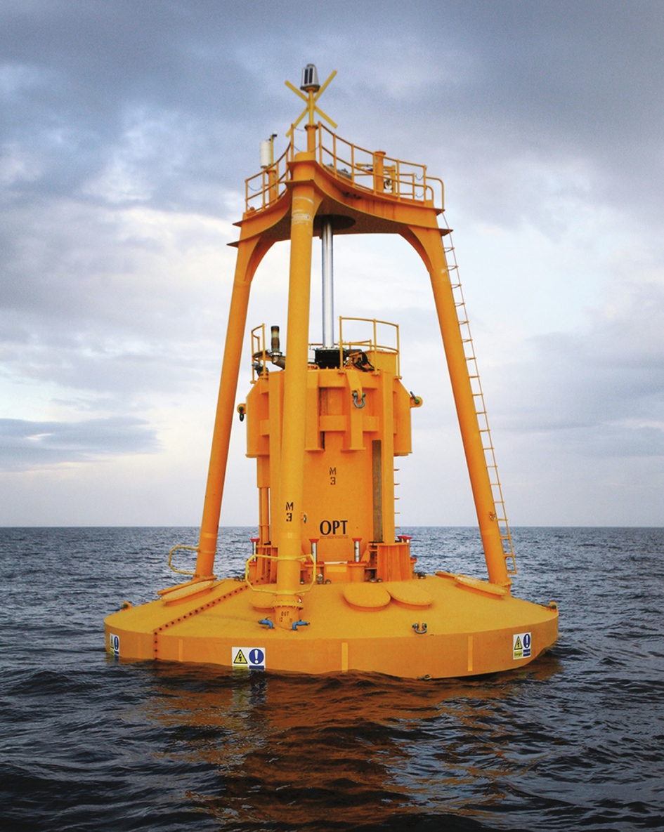
Surface point absorbers are floating structures that absorb wave energy from all directions (i.e. in contrast to an attenuator device). Point absorbers have relatively small dimensions relative to typical wavelengths, and so have diameters of a few metres. Examples of point absorbers are WaveBob and PowerBuoy (Fig. 5.11).
Oscillating Wave Surge Converter
Oscillating wave surge converters (OWSCs) are formed of near-surface collectors mounted on an arm pivoted near the seabed. The arm oscillates as an inverted pendulum due to the movement of water particles in the waves. These devices are also known as inverted pendulums. A well-known example of an OWSC is the Oyster.
Oscillating Water Column
Oscillating water column (OWC) devices are partially submerged, hollow structures, open to the sea below the water surface so that they contain air trapped above a column of water. Waves cause the column to rise and fall, acting like a piston, compressing and decompressing the air. The air is channelled through an air turbine to generate electricity. One example OWC is the Limpet.
Overtopping Devices
Overtopping devices consist of a wall over which the waves wash, collecting the water in a storage reservoir. The incoming waves create a head of water, which is released back to the sea through conventional low-head turbines installed at the bottom of the reservoir. An overtopping device may use collectors to concentrate wave energy. An example of an overtopping device is the Wave Dragon.
5.4.2 Comparison Between WEC Technologies
Issues associated with WECs are survivability (because they will generally be sited in locations where the wave climate is, by its very nature, extreme), and the cost associated with designing the devices to survive such conditions. As an example of the scale of these devices, data extracted from Previsic [12] provides a comparison (Table 5.3).
Table 5.3
| Technology | Length or Height (m) | Width or Diameter (m) | Weight (tonnes) | Rated Power (kW) |
|---|---|---|---|---|
| Pelamis | 180 | 6 | 680 | 750 |
| Power Buoy | 10 | 11 | 136 | 150 |
| Wave Dragon (48 kW/m) | 220 | 390 | 49,000 | 12,000 |
| Oyster | 13 | 26 | 408 | 800 |

The scale is immense—every kilowatt of rated power requires around 0.7 tonnes of steel.2
5.4.3 Basic Motions of WECs
An object, which is floating on the water surface, or submerged underwater, generally has six degrees of freedom—provided that no constraint prevents its motion. It can translate along or rotate around the three major axes. Assuming that waves are propagating along the x axis (Fig. 5.1), the three translational motions are called, surge (x), sway (y), and heave (z). The rotational motions are called rolling, pitching, and yawing around x, y, and z axes, respectively.
5.4.4 Theory of Heaving Point Absorbers
Mass-Spring-Damper
The motion of a WEC can be simplified and studied using vibration theory. In general, most vibrational motions can be simulated/explained by the balance of a restoring force, a damping force, and external forces acting on a body. Depending on the nature of the external forces, a vibration can be periodic or random, similar to what we saw in wave theory (i.e. regular and random waves).
Assuming just one degree of freedom for motion (e.g. a heaving point absorber), the equation of motion can be written as
∑F=maz=−ksz+Fdamp+Fext(t)
where ks is the spring constant, m is the mass, and az is acceleration, and Fdamp and Fext are damping and external forces, respectively. The damping force is usually proportional to the velocity and is expressed as cduz=cddzdt![]() , where cd is velocity in the z direction. The spring force is the restoring force, which is a combination of Archimedes/Buoyancy force and gravity, which tends to return the system to its equilibrium position. Therefore, the single degree of freedom (SDOF), mass-spring-damper equation can be written as
, where cd is velocity in the z direction. The spring force is the restoring force, which is a combination of Archimedes/Buoyancy force and gravity, which tends to return the system to its equilibrium position. Therefore, the single degree of freedom (SDOF), mass-spring-damper equation can be written as
md2zdt2+cddzdt+ksz=Fasin(ωFt+ϕ)

Note that in the earlier equation, we assumed that the external force is a simple harmonic force with an amplitude of Fa and angular frequency of ωF. This makes sense if we assume that the force is generated by a harmonic wave. Eq. (5.51) is a linear ordinary differential equation, and so can be solved analytically. The solution can be found by replacing z = zoeξt into the earlier equation, where zo is a constant.
Analytical Solution of Free Vibration
First, consider a case where the external force is zero. We refer to that case as free vibration. This will be equivalent to a WEC in a calm sea, which is displaced from its equilibrium position. It will gradually be brought back to its equilibrium position after a few oscillations. The governing equation for free vibration reduces to
md2zdt2+cddzdt+kz=0
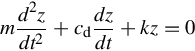
Replacing zoeξt into the previous equation, leads to
{mξ2+cdξ+ks}zoeξt=0
Because zoeξt is not zero, mξ2 + cdξ + ks should be zero. Using the quadratic formula, the solution becomes
ξ=−cd±√c2d−4mks2mandΔ=c2d−4mks
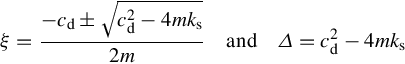
Consider a special case, where there is no damping (undamped system: cd = 0). For an undamped system,
ξ=0±√0−4mks2m=√−ksm=i√ksm=iωN→z=zoeiωNtor using the Euler’s formulaz=zocos(ωNt+go)
where i=√−1![]() and ωN=√km
and ωN=√km![]() is the natural frequency of the system. This is equivalent to having a WEC in a calm sea with no damping. When it is displaced from the equilibrium position, the system oscillates indefinitely. The solution for an undamped system is a simple harmonic equation (i.e. z=zocos(ωNt+go)
is the natural frequency of the system. This is equivalent to having a WEC in a calm sea with no damping. When it is displaced from the equilibrium position, the system oscillates indefinitely. The solution for an undamped system is a simple harmonic equation (i.e. z=zocos(ωNt+go)![]() ), where the amplitude (zo) and phase (go) of this harmonic motion depend on the initial condition.
), where the amplitude (zo) and phase (go) of this harmonic motion depend on the initial condition.
When damping is significant, depending on the sign of the Δ in Eq. (5.54), we have three cases as follows (see Fig. 5.12):
- • Δ < 0 or cd<2√mk
 or cd < 2mωN: underdamped system; in this case the system will oscillate, but its amplitude gradually decreases until it rests. In the undamped system that we considered first, also Δ < 0, and the system oscillates; however, the amplitude does not decrease, and theoretically never stops oscillating.
 - • Δ > 0: overdamped system; due to high friction, the system cannot oscillate and returns to equilibrium quickly.
- • Δ = 0 or c*d=2√mk
 : critically damped; where cd* is defined as the critical damping coefficient. In this case, the system cannot oscillate and quickly returns to equilibrium, similar to the overdamped system.

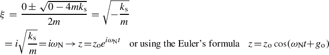
WECs, in general, are underdamped. In the absence of external wave forces, a WEC will oscillate and gradually stop due to frictional damping. The solution of an underdamped system can be found using Eq. (5.54). In order to better formulate the solution, we define the damping ratio (ζ) as
ζ=cdc*d=cd2mωN=cd2√mk→ζ<1≡Δ<0

Using Eq. (5.54) and the previous definitions for damping ratio and natural frequency, it can easily be shown that
ξ=−ζωN±(√−1√1−ζ2)ωN
and the solution of an underdamped system becomes
z=zoeξt=zoe−ζωNtcos(√1−ζ2ωNt+g1)

where zo and g1 are constants, and depend on the initial conditions. When the damping ratio is zero, the previous solution reduces to an undamped system (Eq. 5.55). When the damping ratio is between 0 and 1 (i.e. underdamped system), the term e−ζωNt![]() leads to an exponential decay of the amplitude as can be seen in Fig. 5.12. Finally, when the damping ratio is 1 (i.e. critically damped), the solution is zocos(g1)e−ζωNt
leads to an exponential decay of the amplitude as can be seen in Fig. 5.12. Finally, when the damping ratio is 1 (i.e. critically damped), the solution is zocos(g1)e−ζωNt![]() , which is an exponential decay line.
, which is an exponential decay line.
Analytical Solution of Forced Vibration
In the presence of an external force, the solution of the differential equation is a combination of the solution for free vibration and a particular solution. In the theory of ordinary differential equations, the solution of the free vibration (RHS = 0) is also called homogeneous solution, and the forced vibration is called nonhomogeneous solution (RHS ≠ 0).
In a similar way to free vibration, the solution of the forced vibration case (Eq. 5.51) can also be found by replacing z=z1eξt=z1eiωFt![]() or z=z1sin(ωFt+gF)
or z=z1sin(ωFt+gF)![]() . Note that here the solution frequency is ωF, which is the frequency of the external force. We do not present the steps for this case, as it is very similar to what we saw in the free vibration case.
. Note that here the solution frequency is ωF, which is the frequency of the external force. We do not present the steps for this case, as it is very similar to what we saw in the free vibration case.
z=z1sin(ωFt+gF)wherez1=Fa√m2(ω2N−ω2F)2+(cdωF)2andtangF=−cdωFm(ω2N−ω2F)

In the previous equation, z1 is the amplitude of the vibration or response of the system to the external forcing. As we can see, this amplitude is dependent on the frequency of the external force compared with the natural frequency of the system, and also the damping coefficient. For instance, we can see that as ωF approaches ωN, the denominator becomes smaller (ω2N−ω2F→0![]() ), and this leads to a larger response amplitude. Also, a larger damping coefficient leads to an increase of the denominator or smaller amplitude.
), and this leads to a larger response amplitude. Also, a larger damping coefficient leads to an increase of the denominator or smaller amplitude.
To perform a more quantitative analysis, let us reformulate the amplitude in Eq. (5.59) as follows (by replacing cd=2ζ√km![]() , Eq. (5.56),
, Eq. (5.56),
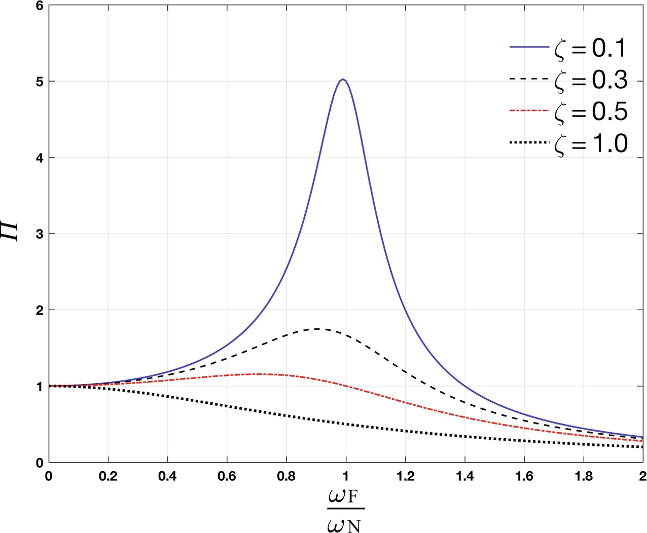
z1=Fa/ks√(1−ωFωN2)2+(2ζωFωN)2=Fa/ks×Π
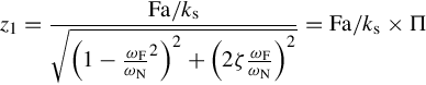
The numerator of the previous equation (Fa/ks) is constant, but the denominator depends on the frequency of the forcing function and damping ratio. Fig. 5.13 shows how the frequency of the external forcing and damping ratio affects the amplitude of the response function. For an energy absorber, the extracted energy would be proportional to the square of the amplitude (i.e. z21![]() ) as we will discuss later. Therefore, it is essential that the frequency of the external forces (i.e. waves) are close to the natural frequency of the energy absorber. This will lead to an important topic of phase control and added mass, which is discussed briefly in the next section.
) as we will discuss later. Therefore, it is essential that the frequency of the external forces (i.e. waves) are close to the natural frequency of the energy absorber. This will lead to an important topic of phase control and added mass, which is discussed briefly in the next section.
Simple Model of a Heaving Point Absorber
Now, consider a simple model of a heaving point absorber as shown in Fig. 5.14. The list of forces acting on the point absorber can be summarized as follows:
mdz2dt2inertia=Fwaves+Frestoring+{Fhydrodynamicdamping+Fpower take-off}+Ftuning/addedmass
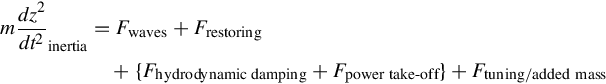
- • Inertia force is proportional to the mass of the floating body.
- • Hydrostatic and gravity forces act as a restoring force.
- • Damping force: a combination of hydrodynamic damping and power take-off force.
- • External force exerted by waves and has a harmonic or random nature.

The previous forces should be formulated using wave theories, or simulated using CFD models.
Considering the simple case of linear wave theory, we start by formulating damping forces. Imagine a heaving point absorber which oscillates in still water—the oscillation can begin with an initial displacement of the point absorber from its equilibrium position. If no external force is applied to the point absorber, it will gradually lose its energy and stop after a few oscillation cycles. During oscillation, waves are radiated from the object. These radiated waves are taking energy off the point absorber. According to linear wave theory, the radiating force can be approximated as follows
Frad=−(maddaz+bhduz)=−(maddd2zdt2+chddzdt)
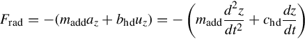
in which the force consists of two parts: added mass inertial force and hydrodynamic damping force. The added mass madd and bhd are dependent on the shape of the point absorber. They are determined by experiment or numerical simulation.
To formulate the restoring force, assume that there is no wave (calm sea) and the point absorber is in equilibrium. The downward force is the weight of the point absorber, and the upward force is the hydrostatic pressure or Archimedes force. When the point absorber is displaced from its equilibrium position, the difference of the Archimedes force and weight tends to bring the system back to equilibrium, and acts as a spring. If the displacement from the equilibrium position is denoted by z, the restoring force would be equal to the mass of the displaced water according to Archimedes law. If the cross-sectional area of the point absorber is Aa (waterline area), the weight of the displaced water, or the restoring force, would be
Fs=−mg=ρVdg=−ρAazg=kszandks=ρAag
The power take-off force, which is used to generate electricity, can be linearly formulated similar to a damping force as follows:
Fpower take-off=−cptodzdt
To have more control on the vibration of the point absorber, and to maximize the energy output, we can use tuning or an additional added mass. By using this additional mass, we can change the natural frequency of the system and control the phase lag between the vibration of the point absorber and waves. The inertia force of this additional mass is
Ftuning=mtundz2dt2
Replacing all forces into Eq. (5.61), leads to
mdz2dt2=Fwsin(ωFt+gF)−ksz−{[maddd2zdt2+chddzdt]+cptodzdt}−mtundz2dt2

which after rearranging becomes
{m+madd+mtun}dz2dt2+{bhd+bpto}dzdt+ksz=Fwsin(ωFt+gF)

As we can see, the previous equation is exactly equivalent to Eq. (5.51). We can use a similar solution as presented in Eq. (5.59) to find the amplitude and phase of the motion for the point absorber. In order to find the solution, we just need to replace mass (m) with total mass (m + mtun + madd), and the damping coefficient with cpto + chd.
5.5 Wave Resource Assessment
For tidal resource assessment, it is generally sufficient to measure and analyse3 the resource over a relatively short timescale (e.g. 30 days) in order to quantify the resource over a much longer time period (e.g. >1 year). In addition, there is minimal interannual variability in the tidal resource,4 and so the Annual Energy Yield (AEY) for 1 year will generally provide a good estimate of the AEY for any year. By contrast, waves exhibit variability over a wide range of timescales, from storm (<24 h), to seasonal, and interannual variability. It is therefore essential that any wave resource assessment captures this range of timescales.
Gunn and Stock-Williams [13] analysed 6 years of NOAA WaveWatch III model output to assess the ‘theoretical’ global wave energy resource (Fig. 5.15). Spatial data of this form, including regional studies at higher resolution [14], are useful for providing an overview of which areas are energetic (e.g. the North Atlantic—Fig. 5.15), and so represent a good opportunity for wave energy conversion, and which regions are less energetic (e.g. the Arabian Sea). Further, many regions, setting aside any practical constraints, can perhaps be identified as being too energetic, for example, much of the Southern Ocean, where the wave climate would present significant challenges to device survivability (see Section 5.5.2). However, spatial resource assessments of mean wave conditions, even when based on relatively long-time periods (e.g. 6 years used to compile Fig. 5.15), do not give potential developers and investors sufficient information about temporal variability.

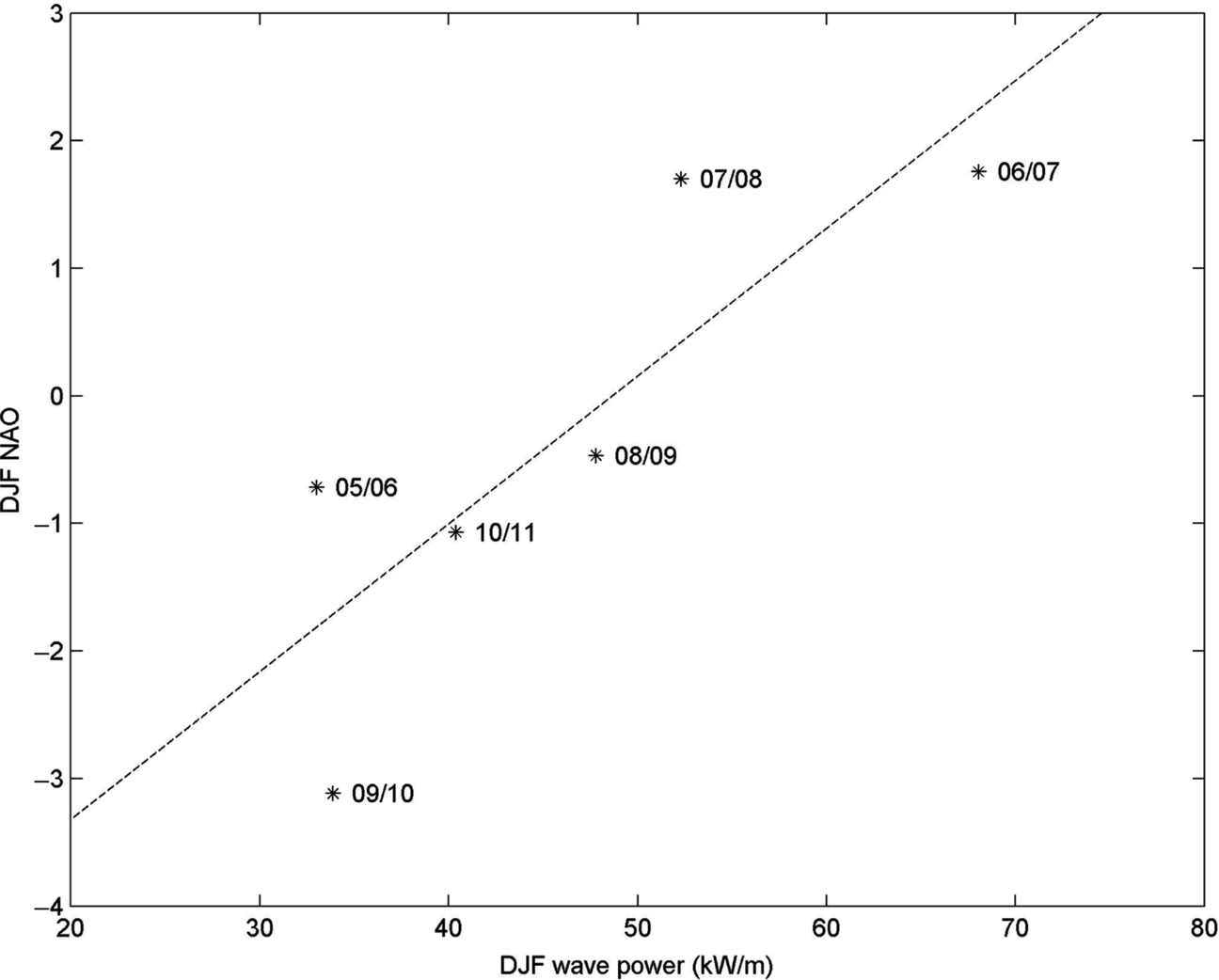
Temporal wave resource assessment can be performed directly either from observations or from examining time series generated by (validated) numerical models. The problem with relying on instrumentation, for example, directional wave buoys (Section 7.2.1), is, in addition to cost, potential limitations on the length of the deployment available for subsequent analysis. For example, in northwest Europe, it is generally considered that a minimum of around 7 years of data would be required to capture the interannual variability described by the North Atlantic Oscillation (NAO)—a large-scale mode of natural climate variability that has important impacts on the climate of northern Europe [15] (Fig. 5.16). Further, limited measurements during summer months, for example, cannot be used to infer winter wave conditions due to strong seasonal trends in wave conditions. Although it is important to have local measurements of waves to characterize the resource, in many circumstances it is more usual for limited wave buoy observations to be used to validate a numerical model. The numerical model can then be used to assess the wave resource over much longer timescales.
5.5.1 Theoretical, Technical, and Practical Resources
A wave resource assessment of the type presented in the previous section is what is known as a ‘theoretical resource’ assessment. A theoretical resource assessment estimates the annual average energy production for a specific wave (or tidal) resource, and is generally based on numerical modelling, with limited validation from historical data records. By contrast, the ‘technical’ resource is defined as the portion of the theoretical resource that can be captured using a specified technology. It therefore includes device characteristics (e.g. efficiency) and constraints such as interdevice spacings. The calculation of the technical wave resource requires access to a power matrix for the selected technology (e.g. Fig. 5.17). A comparison between the theoretical resource and the technical resource (based on a single Pelamis device) at Bernera in the west of Scotland is shown in Fig. 5.18. Although both theoretical and technical resources exhibit strong seasonal and interannual variability, the extremes in the theoretical resource (e.g. regularly over 500 kW/m) are capped by the device characteristics, rated at 750 kW. Out of interest, the capacity factor (see Section 1.5) for the Pelamis device at this location over a decade of simulation is 22%, which is fairly encouraging compared with other renewable technologies (e.g. Table 1.5).


Finally, the practical resource is the portion of the technical resource that is available after considering all constraints such as socioeconomic and environmental factors. The practical resource excludes regions of low power density, regions that are distant from electricity infrastructure, navigation channels, marine protected areas, etc.
5.5.2 Survivability and Maintenance
WECs operating on the water surface are exposed to storms and other extreme events. In particular, high and steep waves, especially breaking waves, are likely to damage WECs. Further, a particular WEC is designed to operate, and convert energy efficiently, over a limited range of conditions (e.g. see the Pelamis power matrix in Fig. 5.17), usually tuned to the most frequent wave conditions that occur at a particular site: extreme waves are not usually within this range. Therefore, it is necessary for most wave devices to have a survival mode; for example, a device could be sunk to a particular depth where wave orbital motion will be reduced (e.g. related to the wave length), or to relax the load on a turbine in an OWC device.
At the other end of the scale, prolonged periods of low wave energy provide opportunities for device maintenance. A site that is consistently energetic may be desirable from theoretical and technical resource perspectives, but is undesirable from a practical resource perspective.