Ocean Modelling for Resource Characterization
Abstract
In situ measurement campaigns are costly, particularly in the environments, which, by their very nature, are characterized by the strong tidal currents or energetic waves that are suitable for generating electricity. Even the best-funded offshore energy operations suffer from logistical difficulties when it comes to making field measurements in remote locations, and where specialist instruments, vessels, and expertise are required to gather, process, and interpret data. In addition, field campaigns take time; for example, several months of data are often required to characterize tidal conditions at a site, and often several years or more of wave data to characterize the interannual and intraannual variabilities in the wave climate. Under many of these circumstances, ocean modelling is a commonly used and economic tool in resource characterization, which can be used to generate long-time series or understand how the resource varies under hypothetical scenarios such as climate change, extreme events, or how the resource will be influenced by energy extraction. Ocean models can be used at all stages of project development, but are particularly useful at the early scoping stages, prior to detailed site selection and investment in costly field campaigns. However, it should be stressed that models are only as good as their input data, and it is always important to parameterize and validate such models with in situ measurements. This chapter will develop your understanding of the terminology and different types of model used for resource characterization, methods of model validation, and limitations to modelling. After studying the chapter, you should be familiar with a wide range of modelling concepts and techniques, and form an appreciation of model preprocessing and postprocessing, and model validation, as well as gaining insights into how ocean models work, rather than treating them as mysterious ‘black boxes’.
Keywords
Ocean modelling; Tidal modelling; Wave modelling; Finite difference; Boundary conditions; Model validation; Galway Bay; Orkney
In situ measurement campaigns are costly, particularly in the environments, which, by their very nature, are characterized by the strong tidal currents or energetic waves that are suitable for generating electricity. Even the best-funded offshore energy operations suffer from logistical difficulties when it comes to making field measurements in remote locations, and where specialist instruments, vessels, and expertise are required to gather, process, and interpret data. In addition, field campaigns take time; for example, several months of data are often required to characterize tidal conditions at a site, and often several years or longer of wave data to characterize the interannual and intraannual variabilities in the wave climate. Under many of these circumstances, ocean modelling is a commonly used and economic tool in resource characterization, which can be used to generate long-time series or understand how the resource varies under hypothetical scenarios such as climate change, extreme events, or how the resource will be influenced by energy extraction. Ocean models can be used at all stages of project development, but are particularly useful at the early scoping stages, prior to detailed site selection and investment in costly field campaigns. However, it should be stressed that models are only as good as their input data, and it is always important to parameterize and validate such models with in situ measurements.
This chapter will develop your understanding of the terminology and different types of model used for resource characterization, methods of model validation, and limitations to modelling. After studying the chapter, you should be familiar with a wide range of modelling concepts and techniques, and form an appreciation of model preprocessing and postprocessing, and model validation, as well as gaining insights into how ocean models work, rather than treating them as mysterious ‘black boxes’.
8.1 Generic Features of Ocean Models
There are many features that are common to the majority of ocean models, for example, grid types, discretization, and boundary conditions; these features are introduced in this section.
8.1.1 Horizontal Mesh Type
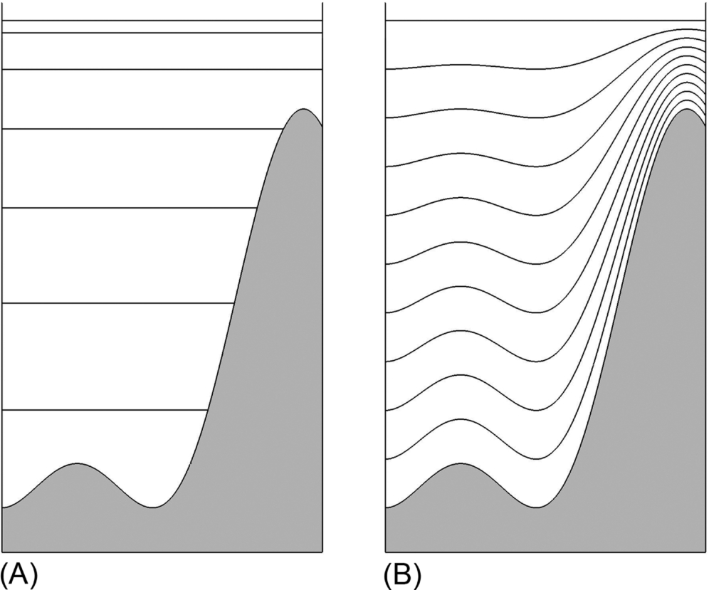
There is a vast array of ocean models, and a wide range of ways in which they can be categorized. There are many places we could begin this classification but, because it is of much interest to wave and tidal resource characterization, we begin by differentiating between structured and unstructured meshes.
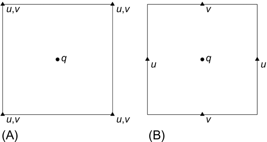
In a structured grid, all grid lines are orientated regularly so that, in a 2D case, the coordinate transformations of curvilinear lines result in a square (Fig. 8.1A). By contrast, this restriction does not apply to unstructured grids (or mesh) (Fig. 8.1B); however, this grid is more complex to deal with numerically. The advantage of a structured grid is its simplicity and ease of preprocessing and postprocessing; however, to achieve a desired resolution (e.g. to resolve the curved geometry shown in Fig. 8.1A), it is necessary to use a constant and high-resolution grid throughout the computational domain. Clearly, this resolution is easier to achieve by spatially varying the grid resolution, as in an unstructured grid (Fig. 8.1B), with the added advantage of lower grid storage (e.g. the circle in the centre of Fig. 8.1, which could represent an island, requires no storage using an unstructured grid).

Within the context of ocean energy, it is clear that due to its ability to accommodate a wide range of scales within a single-model domain, for example, a regional model which incorporates a tidal energy array within a narrow strait, unstructured meshes tend to be favoured for resource assessment. However, many ocean models, particularly 3D models, which simulate a wide range of physical processes, are based on a structured mesh. Under such circumstances, a sequence of nested models, with increasing grid resolution from outer to inner nests, will be required. In general, structured meshes tend to be favoured for larger-scale ocean modelling applications.
8.1.2 Vertical Grid Type
In addition to horizontal resolution, 3D models must also consider the vertical coordinate system. The simplest vertical coordinate system, known as z-coordinates, has been used by the ocean modelling community for many decades. The z-coordinate scheme divides the water column into a fixed number of depth levels, and these can be distributed to provide higher resolution in any particular region, such as the surface layer (Fig. 8.2A). The disadvantage of the z-coordinate system, as demonstrated in Fig. 8.2A, is that it has problems dealing with large changes in bathymetry, which can lead to unrealistic vertical velocities near the bed. Increasing the number of vertical levels will improve the representation of near-bottom flow, but at increased computational cost. This problem is overcome by the sigma coordinate scheme (also known as terrain following coordinate system), where the vertical coordinate follows the bathymetry (Fig. 8.2B). The sigma coordinate system results in the same number of vertical grid points throughout the computational domain, regardless of large changes in bathymetry. The sigma levels do not have to be evenly distributed throughout the water column and could, for example, be more closely spaced near the surface and bed, allowing boundary layers to be better resolved throughout the domain. However, one disadvantage of sigma coordinates is that they can lead to difficulties when dealing with sharp changes in bathymetry from one grid point to another. This can lead to pressure gradient errors, resulting in unrealistic flows [1]. Increased horizontal resolution, or bathymetric smoothing, alleviates the problem.
8.1.3 Sources of Data
As mentioned in the introduction to this chapter, a model is only as good as the data that is used as model input. In addition, data are essential for model validation, which provides confidence in model performance. Model validation is covered in detail in Section 8.5. The main types of data, described in this section, are coastline and bathymetry data, used to set up model bathymetry and mesh, boundary condition data (e.g. astronomical tides), and surface fields such as wind stress and atmospheric pressure.
Coastline Data
The ‘closed’ model boundary is defined by the coastline, and the source of data will depend on model resolution. For example, for a coarse shelf scale model, the GSHHG (Global Self-consistent, Hierarchical, High-resolution Geography Database) intermediate resolution is sufficient for most applications (Fig. 8.3B), whereas a higher-resolution coastline (e.g. GSHHG full or an alternative dataset) may be desired for smaller-scale coastal applications (Fig. 8.3D). In the example shown, the Pentland Firth (the strait between mainland Scotland and the Orkney archipelago) is adequately resolved using the intermediate resolution, whereas the interisland channels are resolved using the high-resolution dataset. In more advanced modelling systems, it is not necessary to clearly define a coastline, as it will change by wetting and drying, and this moving boundary is computed by the model. For those cases, a larger domain that includes bathymetry and topography (e.g. 10 m above MSL) will be used as input.

Bathymetry Data
Although it is possible to generate a model grid using even the coarsest of bathymetric data, it is generally desirable for the resolution of the bathymetry data to match or exceed the model grid resolution. For example, there is little point generating a model that has a grid resolution of 25 m if the available bathymetry for the region only has a resolution of 1 km.
There are a wide range of sources of bathymetry data, which vary in scale and resolution from multibeam surveys (resolution <10 m) to global and regional datasets such as GEBCO (global 1/2 arc-min grid), NOAA bathymetry and global relief, and EMODnet (European 1/8 arc-min grid). In general, gridded bathmetry datasets tend to be suitable for shelf-scale or regional-scale models, whereas high-resolution multibeam data may be required for refined, localized, model studies. Finally, it is important to correct available bathymetry data to the desired model datum, usually mean sea level (MSL). In general, bathymetry data are available relative to the lowest astronomical tide, LAT1 (see Section 3.9), and so accurate information on tidal range is required to correct to MSL.
Boundary Data
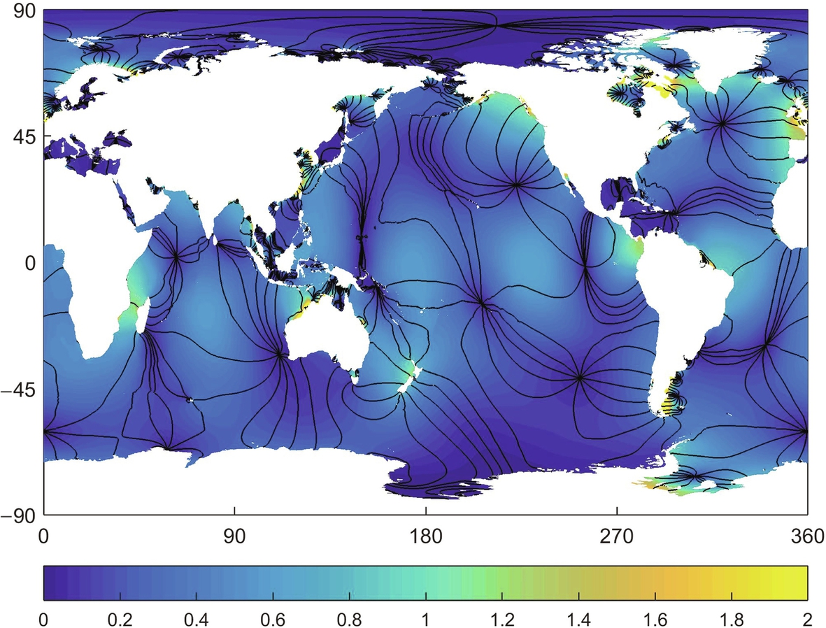
Wave and tidal models require boundary conditions. The models may be nested within a (coarser) outer model domain, which directly transfers information from outer to inner nest (e.g. [2]). However, at some stage, and at some level of nesting, a model will likely require boundary information from an external source. For tidal models, many freely available ‘tidal atlases’ are suitable, such as TPXO. Tidal atlases represent an assimilation between telemetry (satellite) data, in situ data, and global numerical models. One such source, FES2014 [3], is available at a (global) grid resolution of 1/16 × 1/16 degrees for 32 tidal constituents, for both surface elevations and tidal currents, as both amplitude and phase components (Fig. 8.4). For wave models, although there are various wave products, which provide statistical wave properties (e.g. NOAA Wavewatch III which provides Hs and Tz), it is generally preferable to seek products, or to run simulations, which transfer 2D wave spectra from outer to inner nest (e.g. [4]).
Surface Forcing
Surface fields are required to force tidal models, which simulate nonastronomical processes (e.g. wind-driven currents or surge), and wind fields are generally essential to force wave models at all but the smallest of scales (where lateral boundary data may suffice). Many sources of gridded meteorological data are available for model forcing, and two of the most popular products are ERA-Interim (European Centre for Medium Range Weather Forecasting [ECMWF]) and CFSR (National Center for Atmospheric Research/University Corporation for Atmospheric Research [NCAR/UCAR]). Both are reanalysis products—an assimilation of historical observational data, using a consistent assimilation (or ‘analysis’) scheme throughout. By way of example, a snapshot of an ERA-Interim wind field is shown in Fig. 8.5, along with the grid points of the forced wave model for both outer (North Atlantic) and inner (North of Scotland) nests. Unless there are strong topographic effects (e.g. wind that is channelled through a narrow strait), it is generally possible to interpolate relatively coarse wind fields to the ocean model grid points. Another consideration is temporal resolution of the surface fields. In general, 3h wind fields are required to adequately simulate waves. However, for tidal models which include wind-driven currents and surge (in addition to astronomical tides), 6h forcing may suffice.
8.1.4 Time Step
One of the most important considerations in model setup is the time step of the simulation. When selecting a model time step, it is important to consider accuracy, stability, and computational cost. For example, the model time step must be sufficiently small to capture temporal variability in the physical process. An example of this is shown in Fig. 8.6 where, graphically, a time step of Δt = π/8 is insufficient to capture the physical process, but a time step of Δt = π/16 is sufficient. However, more likely, it is stability which constrains model time step. In most practical ocean models, a wave (e.g. phase speed) is travelling across a discrete spatial grid. To ensure stability, the time step must be less than the time it takes for the wave to travel between adjacent grid points. This condition is known as the Courant-Friedrichs-Lewy (CFL) condition. For example, if the phase speed of a 1D tidal simulation, with grid spacing Δx, is ![]() , then the model time step Δt must satisfy
, then the model time step Δt must satisfy

For a typical shelf sea water depth h = 50 m, phase speed c = 22.1 m/s. Therefore, for a typical model grid spacing of Δx = 200 m, time step Δt ≤ 9 s, that is, considerably less than any constraint likely to be imposed by accuracy.

Note that halving of the grid spacing requires a halving of the model time step (Eq. 8.1). However, for a 2D modelling problem, halving the grid (in both x- and y-directions) results in a quadrupling of the number of computational grid points. Because the model time step is halved, the computational cost of the problem will have increased by a factor of 8! Both grid spacing and time step are therefore very important criteria when embarking on a model study. Note that the stability of some numerical methods (called implicit schemes) is not controlled by the CFL criteria. For example, this is the case for the SWAN wave model. Implementing implicit numerical schemes in ocean models is usually challenging. For a model that is unconditionally stable, accuracy becomes the limiting factor.
8.1.5 Staggered Grids
Staggered grids are a simple way of avoiding odd-even decoupling between modelled velocity and scalar fields. It also reduces the computational cost, as it is not necessary to compute all variables at all nodes. Odd-even decoupling is a discretization error that can occur on collocated grids, and leads to classical ‘checkerboard’ patterns in the numerical solution. Ocean models tend to be based on two staggered grid arrangements: the Arakawa B-grid and the Arakawa C-grid (Fig. 8.7). The u and v components in an Arakawa B-grid are computed at the same location (Fig. 8.7A). Because the u (or v) momentum equation contains a v (or u) velocity in the Coriolis term, an Arakawa B-grid is suitable for problems in which the geostrophic balance is important. By contrast, an Arakawa C-grid is good for tidal problems, because velocity points are located midway between the elevation points. Because the flow is driven by the surface slope (e.g. ∂η/∂x, ∂η/∂y), this avoids the need to interpolate elevations.
Most popular finite difference models used for resource assessment use a C-grid arrangement (e.g. ROMS and POM). Incidentally, the simplest grid arrangement, a collocated grid, where velocity and scalar fields are calculated at the same grid points, is known as an Arakawa A-grid.
8.1.6 Discretization
Discretization concerns the process of transferring a continuous function into one that is solved only at discrete points. Therefore, mathematical equations such as the ones included in Chapter 2 are continuous, but we must consider them at discrete points (e.g. points in time and space) before they can be solved numerically, that is, via numerical models.
Discretization: A Simple Finite Differencing Example
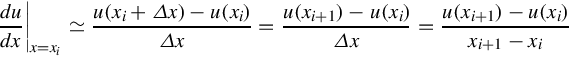
We will demonstrate the concept of discretization using a simple finite differencing example. Consider a thin rod of length L (Fig. 8.8). We wish to know the temperature at each point along the rod. We can denote any position along the rod as x. In mathematical notation
where the variable u is the temperature. Because u(x) is a continuous function, there are an infinite number of points along this rod. However, it is much easier if we consider a finite number of discrete points along this rod. In numerical notation
If we distribute these discrete points uniformly along the rod, the spacing between the grid points will be Δx = L/(N − 1). Consequently,
To find the temperature at each point, we need to solve the following differential equation

where k is a constant and depends on the material property of the rod.
8.2 Numerical Methods
8.2.1 Finite Difference Method
To solve a differential equation like Eq. (8.5), we need to evaluate derivatives. Recalling from calculus (Chapter 2), the derivative of a function is defined as:
From a geometrical perspective, the derivative at a point equals the slope of the tangent line at this point.
As an approximation, the derivative can be estimated as
It is clear that as the number of grid points (N) increases, Eq. (8.7) leads to more accurate values. Referring to the simple rod example, the derivative at a general point xi can be approximated as
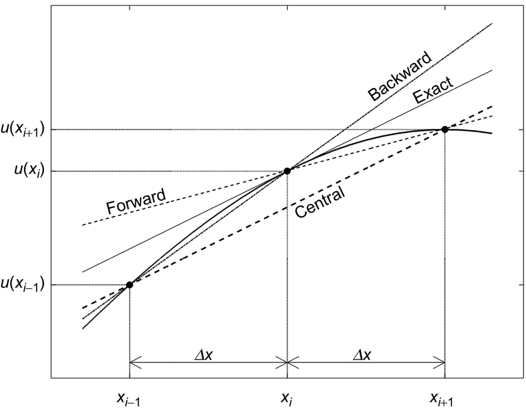
which is called a finite difference. Specifically, a finite difference of the form of Eq. (8.8) is called a forward difference.
Alternatively, if we use function values at grid points xi−1 and xi, we call it a backward difference:

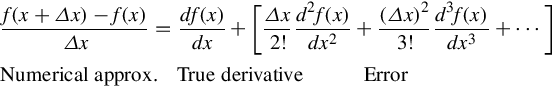
Another form is the central difference and, as shall be shown in the next section on truncation error, it is more accurate than either backward or forward difference. It is defined as

Fig. 8.9 shows the geometrical interpretation of central, forward, and backward finite difference schemes.
Truncation Error
Truncation error is defined as the difference between the true (analytical) derivative of a function and its derivative obtained by numerical approximation.
Beginning with the Taylor series expansion

Suppose that we approximate a derivative using a forward difference scheme of the form given in Eq. (8.8). The Taylor expansion gives
In this case, the truncation error is

Because it involves terms in Δx and higher powers, we say that it is of order Δx, written as O(Δx). Note that as ![]() we obtain the true derivative.
we obtain the true derivative.
The backward difference scheme given by
also has an error O(Δx).
A better approximation can be obtained using the central difference scheme
From the Taylor series expansion we obtain

Hence, by subtracting Eq. 8.16 from 8.11
for the central difference scheme. In this case, the error is O(Δx2). Because Δx is small, Δx2 < Δx. Therefore, a centred scheme has a smaller truncation error (i.e. is more accurate) than a forward or backward scheme.
8.2.2 Finite Element Method
The majority of ocean modelling problems involve complex geometries such as irregular coastlines, inlets, islands, and headlands. Regular (rectangular or curvilinear) grids cannot conveniently resolve these complex geometries. Finite element method (FEM) is based on an irregular (e.g. triangular) mesh that can easily resolve complex geometries (e.g. Fig. 8.1B). FEM originated in the area of solid mechanics to calculate stress and strain in structures. However, it is today applied to a wide range of multiphysics problems, including fluid mechanics and ocean modelling. FEM can be regarded as a general numerical method to solve partial differential equations (PDEs). The implementation of FEM to fluid/solid mechanics problems involves many steps, and a detailed explanation of those steps is beyond the scope of this book. However, the basic concepts of the method are introduced briefly, because many renewable energy problems use FEM codes for numerical simulations. For instance, ADCIRC is an FEM-based ocean circulation model that can be used to simulate the tidal energy resource of a region (e.g. [5]). Also, FEM is a common technique for the analysis of tidal turbine blades or the structural design of ocean renewable energy devices (e.g. [6]).
In FEM, the domain is first discretized into a number of elements (see Fig. 8.10 as an example). These elements are generated such that higher resolution (i.e. smaller element size) is obtained in places of interest (such as near the coastline in Fig. 8.10).

Many types of 2D or 3D elements are common in FEM, such as triangular, quadrilateral, and tetrahedron. The triangular mesh is the most common type. After discretization, the state/dependent variable, u (e.g. water depth, velocity, displacement, stress, etc.) is approximated by a function, ![]() . In other words, u is the exact solution of the PDE of interest, which in most cases does not exist, whilst
. In other words, u is the exact solution of the PDE of interest, which in most cases does not exist, whilst ![]() can approximately satisfy the PDE.
can approximately satisfy the PDE. ![]() is approximated using basis functions
is approximated using basis functions
where ψi denotes basis functions and ui is the approximate value of the state variable at node i. For instance, if an element has three nodes, u can be approximated by
Note that if (x1, y1) is the coordinate of node 1, then basis functions are selected such that ψ1(x1, y1) = 1, ψ2(x1, y1) = 0, and ψ3(x1, y1) = 0. The simplest form of a basis function is the Lagrangian linear function over an element as follows
The coefficients of this function can be found by imposing the conditions explained previously (i.e. ![]() )), that is
)), that is
As a next step, after selecting the basis/shape functions, the unknown values ui should be estimated. FEM forms enough algebraic equations to compute the unknown ui at all nodes by minimizing the error. Let us consider the exact form of a differential equation
where L is a general differential operator (e.g. ![]() ). If we replace
). If we replace ![]() into the differential equation, it will not exactly satisfy it (because
into the differential equation, it will not exactly satisfy it (because ![]() ), and leads to a residual error (R) as follows
), and leads to a residual error (R) as follows
In FEM (weighted residual method), ui is determined such that the residual error is minimized, therefore,
The previous equation is called the weak form of a differential equation, because the integral (some kind of average) of L(u) is set to zero. Ω is the domain of the problem and Wj are the weight/test functions. Depending on the FEM scheme, several types of weight functions are chosen. For instance, in the Galerkin method, weight functions and basis functions are the same (Wj = ψi).
After implementing Eq. (8.26), enough algebraic equations are formed to compute the nodal values of the state variable.
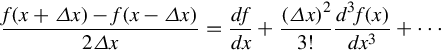
FEM models usually use a simple file format to define the mesh. Fig. 8.11 shows a sample mesh file for the ADCIRC model. As this figure shows, first, the total number of elements and nodes is written. Then, the coordinate of each node in a coordinate system is defined. Each element in a triangular mesh is uniquely defined by connecting three nodes. The state variables are computed at each node (or centre of an element) and can be processed using postprocessing software such as Matlab.
8.2.3 Finite Volume Method
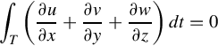
Finite volume method (FVM), like FEM, is based on an unstructured (e.g. triangular) mesh. Therefore, it is suitable for irregular and complex geometries. FVM has another advantage over FEM for fluid mechanic problems. So far, the numerical methods that we presented have been based on PDEs. By contrast, FVM is based on the integral form of the conservation laws, rather than their differential form. This leads to more accuracy/stability, especially for sharp gradients (i.e. large derivatives) inside a domain, which is also called shock-capturing property. To explain this more clearly, as we mentioned before, the dynamics of flow can be described by conservation of mass, momentum, and energy. These conservation laws can be written as a system of PDEs. Alternatively, conservation laws can be expressed by integral equations (i.e. Reynolds transport theorem). For instance, the differential form of the continuity equation can be written as
where u, v, and w are the components of flow velocities in the x, y, and z directions, and ρ is the density. The integral form of continuity for a control volume (or a finite volume) can be written as

where V is the control volume, S is the control surface, u = (u, v, w), and S is the surface vector.
Therefore, the change of mass inside a control/finite volume plus the net mass fluxes through the control surface should be zero. In FVM, the domain is first discretized into a number of nonoverlapping finite volumes or cells (see Fig. 8.12 as an example). Usually, these finite volumes are triangles (2D) or prisms (3D). Next, conservation laws are applied to each individual cell to form enough algebraic equations, which can be solved to compute the state variables.
8.3 Tidal Modelling
There are a wide variety of models available for tidal resource assessment, ranging from open-source to commercial codes, and from 2D structured to 3D unstructured. A summary of the main models that are suitable for tidal resource assessment is provided in Fig. 8.13. These models range in complexity of user operation; for example, POM is a relatively simple code, but requires compilation and execution via line commands, whereas commercial codes such as MIKE 3 are controlled by a graphical user interface (GUI) and are suitable for running on desktop PCs. Some of the models (e.g. ROMS and FVCOM) are rather difficult to install and operate, and are generally recommended for more experienced modellers. However, the advantage of such complexity is the flexibility to couple models such as ROMS to many other models (and multiple models simultaneously), for example, the SWAN wave model, the WRF atmospheric model, and the community sediment transport model. Further, because models like ROMS are suited for parallel processing, they can be implemented on supercomputers (see Section 8.7). This is particularly useful for long timescale (e.g. decadal) and high-resolution simulations, but particularly when the tidal model is coupled with other modelling systems, and hence computationally expensive.

8.3.1 Turbulence Closure
For large Reynolds numbers (>2000), the flow velocity experiences fluctuations around the mean velocity. Common numerical models cannot simulate these fluctuations, because they occur over very small timescales (e.g. fractions of seconds). Alternatively, they replace the velocity by mean and fluctuating components as follows
where ![]() is the time averaged and
is the time averaged and ![]() is the fluctuating part. Tidal models simulate the temporal average rather than the actual velocity (u) to avoid this issue. The argument is that these small and rapid fluctuations in velocity are not important, compared with the mean velocity that is of relevance to tidal energy generation. The time average of the fluctuating velocity is zero. Therefore, if the Navier-Stokes equations were linear, we could just replace velocities by time averaged velocities. To make this point clearer, consider the continuity equation, which is a linear equation. Taking a moving time average leads to
is the fluctuating part. Tidal models simulate the temporal average rather than the actual velocity (u) to avoid this issue. The argument is that these small and rapid fluctuations in velocity are not important, compared with the mean velocity that is of relevance to tidal energy generation. The time average of the fluctuating velocity is zero. Therefore, if the Navier-Stokes equations were linear, we could just replace velocities by time averaged velocities. To make this point clearer, consider the continuity equation, which is a linear equation. Taking a moving time average leads to

Also, for the x component of velocity (and similarly for the other components), we have
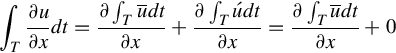
Because the average of the fluctuating velocity is zero, the time averaged continuity equation simply becomes
Unfortunately, this is not the case for the nonlinear parts of the momentum equation. For instance, if we just consider the convective acceleration term in the momentum equation, (see Chapter 2) we have
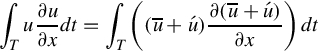
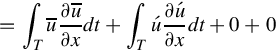
Because the time average of ![]() is not zero (in contrast to
is not zero (in contrast to ![]() ), additional terms appear in the momentum equation. For instance, the convective acceleration term after time averaging becomes
), additional terms appear in the momentum equation. For instance, the convective acceleration term after time averaging becomes

Therefore, additional unknowns (e.g. ![]() ) appear in the governing equations. Because the number of unknowns becomes more than the number of equations after time averaging, the Navier-Stokes equations are no longer closed. This is called the closure problem. Additional equations, called turbulence equations, are added to address this issue, and popular choices in ocean modelling are k-ϵ and the Mellor-Yamada 2.5 scheme (e.g. [9]).
) appear in the governing equations. Because the number of unknowns becomes more than the number of equations after time averaging, the Navier-Stokes equations are no longer closed. This is called the closure problem. Additional equations, called turbulence equations, are added to address this issue, and popular choices in ocean modelling are k-ϵ and the Mellor-Yamada 2.5 scheme (e.g. [9]).
8.3.2 Boundary Conditions
Because we generally simulate a particular region of interest (e.g. part of a bay, estuary, or shelf sea environment), we need to specify the conditions at the boundaries of our modelling domain. These boundaries can be forced by what is happening outside a modelling domain, and therefore models need the boundary information as input data. For instance, tidal waves are generated in the deep oceans by gravitational attractions of the Sun and the Moon, which are usually outside the modelling domain for a tidal project. The tidal forcing data (water elevation and velocity) should be specified at the boundaries of a model. The tidal information data are usually extracted from global tidal models or from a coarser outer modelling domain. Sometimes the boundaries of a model are affected by what is happening inside the domain. For instance, a tidal wave that is propagating towards a coastline may be reflected back into the domain, or can be radiated out from another boundary.
From a mathematical point of view, the values of state variables (e.g. time series of velocities) can be specified at a boundary. These are called Dirichlet boundary conditions. Alternatively, the derivative of a state variable can be specified at a boundary. For example, at a reflective boundary, the derivative of water elevation can be specified as zero. These are called Neumann boundary conditions. In practice, the boundary conditions for a tidal model can be more complex: usually a mix of Dirichlet and Neumann.
There are a variety of types of boundary condition applied to ocean models (e.g. [10]), as follows.
Coastlines
This is a zero gradient condition for surface elevation, and zero flow for the normal component of velocity. For tangential velocities, the coastline can be treated as either no-slip or free-slip, depending on the configuration of the problem; for example, a no-slip condition may have a significant influence on the flow field when simulating strong tidal flows through a narrow strait. Models that simulate a moving boundary (wetting and drying) implement a more complicated and iterative procedure to find the wet part of a domain.
Clamped Elevation
The free surface displacement is set to an externally prescribed value. This is a popular boundary condition for tidal simulations, due in part to the smooth spatial variability of elevation data, and readily available satellite-altimetry-derived data (e.g. Section 8.1.3).
Clamped Normal Velocity
This condition simply sets the normal velocity component in the boundary cell to an externally prescribed value.
Flather
Applied to the normal component of barotropic velocity, the Flather condition is an adjustment to the externally prescribed normal velocity, based on the difference between modelled and externally prescribed surface elevations. This is a form of the classical radiation boundary condition.
Chapman
The corresponding boundary condition for water elevation (assuming an outgoing signal) is Chapman.
8.3.3 Time Splitting
The presence of a free surface in a tidal model introduces waves in the domain that propagate at a speed of ![]() . These waves impose a more severe constraint on the model time step than any of the internal processes (Section 8.1.4). Therefore, a split time technique is generally used in 3D modelling. The depth-averaged equations are integrated using a ‘fast’ (barotropic) time step, and the values of
. These waves impose a more severe constraint on the model time step than any of the internal processes (Section 8.1.4). Therefore, a split time technique is generally used in 3D modelling. The depth-averaged equations are integrated using a ‘fast’ (barotropic) time step, and the values of ![]() and
and ![]() used to replace those found by integrating the full equations on a ‘slower’ (baroclinic) time step [11]. In general, it is recommended that the ratio between barotropic and baroclinic time steps is in the range 10–20, but this will depend on the scale of the problem. The purpose of time splitting is to reduce the computational effort, because the 3D time step is considerably more costly than the 2D time step.
used to replace those found by integrating the full equations on a ‘slower’ (baroclinic) time step [11]. In general, it is recommended that the ratio between barotropic and baroclinic time steps is in the range 10–20, but this will depend on the scale of the problem. The purpose of time splitting is to reduce the computational effort, because the 3D time step is considerably more costly than the 2D time step.
8.4 Wave Modelling
There are two main classes of wave models: phase-resolving models and phase-averaged models. In a phase-resolving model, the domain is discretized onto a grid that is relatively fine compared with the wave length, and the vertical displacement of the sea surface calculated in detail. Because such a process is computationally expensive, phase-resolving models tend to be applied to relatively limited domains, and are most appropriate in cases of strong wave diffraction and reflection due to coastal structures. Examples of wave resolving models are SWASH [12], CGWAVE, and FUNWAVE [13]. Although such models could be useful for wave resource characterization, they are not generally used due to very high computational cost; therefore, the remainder of this section concentrates on the more widely applied phase-averaged models.
8.4.1 Phase-Averaged Wave Models
As discussed in Chapter 5, a wave field can be considered as a wave spectrum, which can be represented by a large number of regular sinusoidal wave components. Wave models work by predicting each of these independent wave components individually, and how they vary in space and time, through the energy balance equation, which has the form (e.g. [14])
where E is the spectral energy density, σ is the angular wave frequency, θ is wave direction, x and y are the horizontal dimensions, t is time, and S are the source terms, comprising generation, wave-wave interaction, and dissipation.
Energy density E is not preserved in the presence of ambient currents, and so wave models tend to solve the action density (N) balance equation, where N = E/σ. In spherical coordinates, this can be written as [15]
where cλ and cϕ are the propagation velocities in the zonal (λ) and meridional (ϕ) directions, and cσ and cθ are the propagation velocities in spectral space.
The numerical solution of Eq. (8.39), without any prior assumption about the spectral shape, is what is known as a third-generation wave model [16], and is the most popular type of wave model in use today for resource assessment, including the models SWAN [15], WAM [16], and WAVEWATCH III [17].
8.4.2 Source Terms
Central to third-generation wave models is the calculation of the source terms (RHS of Eq. 8.39), and the key processes are introduced briefly as follows.
Wind Input
There are two mechanisms that describe the transfer of wind energy and momentum into the wave field. Small pressure fluctuations associated with turbulence in the airflow above the water surface are sufficient to induce small perturbations on the sea surface, and to support a subsequent linear growth as the wavelets move in resonance with the pressure fluctuations [18]. This mechanism is only significant early in the growth of waves on a relatively calm sea. When the wavelets have grown to a sufficient size to start affecting the flow of air above them, most of the development commences. The wind now pushes and drags the waves with a vigour that depends on the size of the waves themselves, in a phase known as exponential wave growth. Wave growth can therefore be described as a sum of linear (A) and exponential (BE) growth terms
A drag coefficient is used to transform the wind speed (usually defined at 10 m elevation) into a friction velocity U*, after which a linear expression can be used to calculate A (e.g. [19]), and an exponential expression to calculate B (e.g. [20]).
Dissipation
In deep water, energy is dissipated from the wave field mainly through wave breaking (whitecapping). In shallow water, it may also be dissipated through interaction with the sea bed (bottom friction) and through depth-induced wave breaking.
Whitecapping is active in wind-driven seas, and is the least understood of all processes affecting waves [14]. A complicating factor is that there is no generally accepted precise definition of breaking and, as you can imagine, quantitative observations of deep water wave breaking are very difficult to achieve. However, the whitecapping source term tends to be based on the theory of Hasselmann [21], in which each white-cap acts as a pressure pulse on the sea surface, just downwind of the wave crest.
In water of finite depth, wave energy is dissipated due to interaction with the sea bed, and this tends to be dominated by bottom friction [22]. This can be expressed as [23]

where Cb is a bottom friction coefficient.
As waves propagate from deep to shallow water, wave shoaling leads to an increase in wave height. Waves tend to steepen at the front and to become more gently sloping at the back, and at some point the waves will break. There are various definitions of wave breaking; for example, breaking occurs when the particle velocities at the crest exceed the phase speed, or when the free-surface becomes vertical. Depth-induced wave breaking is included as a source term in third-generation wave models.
Nonlinear Wave-Wave Interactions
Nonlinear wave-wave interactions redistribute wave energy over the spectrum, due to an exchange of energy resulting from resonant sets of wave components. There are two processes that are important for the inclusion of nonlinear wave-wave interactions in wave models: four-wave interactions in deep and intermediate waters (known as quadruplets) and three-wave interactions in shallow water (triads). A good explanation of the principal of nonlinear wave-wave interactions is provided by Holthuijsen [14]. Two wave paddles, generating waves of different frequencies and directions, are placed in two corners along one side of a tank of constant water depth. The resulting waves create a diamond pattern of crests and troughs, which has its own wave length, speed, and direction. This diamond pattern would interact with a third-wave component, if this third wave had the same wave length, speed, and direction as the diamond pattern. This is the triad wave-wave interaction, which redistributes wave energy within the spectrum due to resonance. Although each of the individual wave components can gain or lose energy, the sum of the energy at each point in the tank would remain constant. In deep water, it is not possible to meet these resonant conditions (i.e. matching of wave speed, length, and direction), and so triad wave-wave interactions cannot occur in deep water. However, in deep water it is possible for a pair of wave components to interact with another pair of wave components in a quadruplet wave-wave interaction.
Quadruplets transfer wave energy in deep water from the peak frequency to lower frequencies, whereas triads transfer energy from lower to higher frequencies, and transform single-peaked spectra into multiple-peaked spectra as they approach the shore. Both are included as source terms in third-generation wave models, and it is noted that both are computationally expensive. Triads, in particular, are often omitted in wave model simulations, whereas quadruplets are often included. For example, in the SWAN wave model, quadruplets are activated by default in third-generation mode, whereas triads are not included by default.
8.5 Validation
According to the statistician George Box, ‘all models are wrong, but some are useful’. Models, however sophisticated, are a representation of reality. To provide confidence in how accurately a model has simulated reality, it is necessary to perform model validation. Of course, validation depends upon the availability of suitable in situ data. Although it is often desirable for such data to be focussed in the region of interest, for example, at the approximate location of a proposed wave or tidal energy array, this is not compulsory. If a model performs well in one region, or under one set of conditions (e.g. during a spring tide), this gives confidence in model performance in another region, or under another set of conditions (e.g. during a neap tide). This is provided that the model parameterizations (e.g. drag coefficient and eddy viscosity) are physically realistic, and the model has not been excessively tuned to fit data in one region or under one unique set of conditions.
8.5.1 Validation Metrics
Various metrics can be used to quantify model validation (e.g. [24]), and some of the most popular metrics are presented in this section.
Correlation Coefficient
Correlation measures the direction and strength of the linear relationship between two variables. If we have a set of n observed (Oi) and simulated (Si) values, the linear correlation coefficient (r) (also known as Pearson’s r) can be calculated as

For a perfect model, r = 1, whilst for a completely random prediction r = 0.
The square of the correlation is often used as a metric, because r2 indicates the proportion of the variance in the observation that can be predicted by the model.
Root Mean Squared Error
Root mean squared error (RMSE) is the square root of the mean of the square of all of the error. The use of RMSE is very common, and it is considered an excellent general-purpose error metric for numerical predictions.
where Oi are the observations, Si predicted values of a variable, and n the number of observations available for analysis. RMSE is a good measure of accuracy, but only to compare prediction errors of different models or model configurations for a particular variable and not between variables, as it is scale-dependent.
Scatter Index
Scatter index (S.I.) is simply the RMSE (Eq. 8.43) divided by the mean of the observations and multiplied by 100 to convert to a percentage error. As an example of the worth of S.I., if an RMSE for significant wave height is 1 m, this gives us no sense of how well the model is performing, because the mean of the observations could, for example, be either 1 m (S.I. = 100%) or 5 m (S.I. = 20%).
Bias
Bias (also known as mean error) is the mean of the simulated values of the selected variable minus the mean of the observed values, that is
It is an index of the average component of the error [25], with a value closer to zero indicating a better simulation This index shows if a model is in general overestimating or underestimating.
Examples of validation metrics applied to a case study of Galway Bay are given in Section 8.9.1.
8.6 Tools for Model Preprocessing and Postprocessing
Preprocessing is one of the most important steps in ocean modelling. Once sources of data have been assembled for model setup (e.g. Section 8.1.3), the model grid and boundary conditions need to be prepared. There are a wide variety of tools which can be used to help set up model grids and boundary conditions, but the two that will be introduced here are Matlab and Blue Kenue.
8.6.1 Matlab
Matlab is a computing environment with a GUI and its own unique, and relatively easy to learn, programming language. An example screenshot of Matlab is shown in Fig. 8.14. Although commands can be entered directly into the Command Window, Matlab is at its most powerful when a Matlab script (i.e. a computer program) is developed and saved in the Editor Window for subsequent execution—an example of which is shown in Fig. 8.14 (this is actually part of the code use to create Fig. 8.7). Matlab is relatively easy to learn, perhaps in contrast to more traditional programming languages such as FORTRAN, as the generated variables instantly appear, and can be visualized, in the Workspace. This aids any necessary debugging, and is particularly useful for the novice user. Matlab also comes with excellent help features linked to extensive documentation.

One of the key advantages of Matlab is that it is widely used by ocean modellers around the world; hence many existing scripts can be shared and downloaded. For example, Mathworks File Exchange2 is a forum for finding and sharing custom Matlab applications, classes, code examples, drivers, functions, and scripts, many of which will be useful for model preprocessing and postprocessing. In addition, various researchers have written preprocessing and postprocessing tool boxes in Matlab for some of the most popular ocean models, for example, ROMSTOOLS3 for setting up and analysing the outputs of ROMS simulations, and OpenEarth tools4 for setting up and analysing the outputs of the SWAN wave model. Further, many excellent packages have been written and are freely available for Matlab, such as the popular t_tide (tidal harmonic analysis) and m_map (mapping toolbox, which has been used to generate Fig. 8.3, for example). Matlab is preinstalled with netCDF libraries—a self-describing file format that is popular for storing numerical model inputs and outputs. Because Matlab is based on the principal of matrices, it excels at setting up and analysing structured grids. However, for unstructured meshes, an alternative software package is recommended—Blue Kenue.
8.6.2 Blue Kenue
Blue Kenue is a freely available preprocessing, analysis, and visualization tool that is suitable for a wide range of model applications, and in particular mesh generation for FEM or FVM models. The interface is very intuitive and easy to use (Fig. 8.15), and Blue Kenue is setup to directly import/export data from/to Telemac and ADCIRC—two very popular unstructured models. Blue Kenue is very flexible and can handle a wide range of data types, including GIS files, GRIB, x−y scatter data, and time series. However, one of the disadvantages of Blue Kenue, in comparison to computing environments which incorporate a programming language like Matlab, is that although you can save all the variables in the workspace as you proceed, it is not possible to save a ‘line-by-line’ sequence of commands. Therefore, if one develops a model grid of a region and wishes to go back several steps in the processing (e.g. to remove an island from the domain), many procedures must be repeated manually, rather than editing and running a script. Note that although primarily used to deal with unstructured (triangular) meshes, Blue Kenue will also generate rectangular meshes. Blue Kenue also has a very easy to implement presentation quality animation facility (including flight paths), helping with model visualization.

8.7 Supercomputing
In 1965, Intel cofounder Gordon Moore noticed that the number of transistors per square inch on integrated circuits had doubled every year since their invention. Moore’s Law predicts that this trend will continue into the foreseeable future. We are now in a golden age of scientific computing, when efficient multicore desktop PCs can be purchased at relatively low cost. However, within the context of ocean modelling, supercomputing refers to running a computational task simultaneously (i.e. in parallel) on hundreds or even thousands of processors. Rather than running a job, representing a single computational domain, in series, the computational domain can be decomposed into several subdomains, which can be run together in parallel (Fig. 8.16). Although such a task is possible on a desktop PC for a limited number of processors, it is when a model that has been optimized for parallel processing is divided into several hundred tasks that supercomputing really excels.

The simplest way of preparing a computational domain for parallel processing is through tiling. However, a ‘tile’ that contains mostly land cells will represent a considerably lighter computational task than a tile which contains entirely sea points—a situation that is known as uneven load balancing. Therefore, many models use load-balancing techniques for domain decomposition, as demonstrated in Fig. 8.16 for the POLCOMS model. Each of the 10 nodes (0–9) shown in this example has 10,281–10,366 ‘wet’ grid cells, representing a departure of no more than 0.5% from the mean–excellent load balancing.
If we were to run a serial task 1000 times, for example, with slightly differing initial conditions for each simulation, we would complete our simulations in 1/1000 of the time that it would take to complete the same tasks in series—a considerable time saving, in a situation that is known as ‘embarrassingly parallel’. This would represent perfect ‘linear’ speedup where
However, due to load balancing, I/O, and overheads associated with communication between parallel tasks, speedup for ocean models is nonlinear. For example, for the SWAN wave model applied to Galway Bay (Section 8.9.1), there is very little reduction in completion time once around 96 processors are exceeded. However, a job which uses >96 processors may take considerably longer to schedule, compared with a job which requests less resources.
8.8 CFD Modelling
The dynamics of flow in both large (ocean tides/waves) and small scale (around a device) problems can be simulated by numerical solution of mass, momentum, and energy equations. Computational fluid dynamics (CFD) models (applied to small scales) and ocean models (applied to large-scale oceanic flows) are based on the Navier-Stokes equations. Further, CFD and ocean models use similar numerical techniques such as FDM or FVM. Although, strictly, ocean modelling is a subset of CFD, those working in the field of ocean energy make a clear distinction between what constitutes CFD, and what constitutes ocean modelling. CFD tends to be used for flows that are more isotropic (genuinely 3D) than ocean applications, where the velocities in the horizontal direction are generally greater than the vertical velocities, and CFD will neglect effects of stratification and Earth’s rotation (e.g. Coriolis).
CFD is routinely used to deal with fluid/structure interaction and scenarios where there are strong shocks. The temporal and spatial scales are considerably different between CFD and ocean model simulations. In the latter, timescales of lunar, seasonal, and decadal are not uncommon, whereas CFD models may be dealing with simulation timescales of several seconds to few hours. CFD models will resolve fairly limited spatial scales (albeit at high resolution), such as the diameter of a tidal stream turbine, whereas ocean models are applied to regional (e.g. 10 km) and ocean basin (1000 km) length scales. CFD models usually require a special treatment of the free surface as their moving boundary condition. However, ocean models are usually based on a 2D approximation (depth-averaged) and compute water elevation or free surface as a state variable, more conveniently.
8.9 Modelling Case Studies
To demonstrate some of the principals introduced in this chapter, we examine two modelling case studies—a wave resource model of Galway Bay (Ireland) and a tidal resource model of Orkney (Scotland). We focus on model setup and validation for the Galway Bay case study, and model setup and interpretation of 3D results for the Orkney case study.
8.9.1 Wave Model of Galway Bay (Ireland)
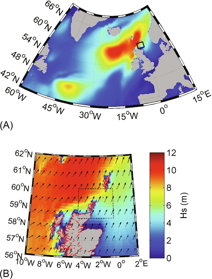
SmartBay5 is Ireland’s national marine test and demonstration facility, suitable for the testing of scaled devices. It is located in Galway Bay, on the west coast of Ireland (Fig. 8.17). The presence of an island chain, the Aran islands, at the entrance to the bay, leads to relatively quiescent wave conditions within the bay, yet a wave climate that is characterized by ‘scaled’ Atlantic conditions [26].

The purpose of this exercise is to describe the setup of a SWAN wave model of Galway Bay, including sources of data, validation, and some results on wave resource assessment.
Model Setup
The model bathymetry was derived from the EMODnet dataset—available at a grid resolution of 1/480 × 1/480 degrees (approximately 200 m) throughout Europe. This bathymetry data was bilinearly interpolated onto a spherical model grid, which covered the inner nested region shown in Fig. 8.17 (which has dimensions approximately 1.0 × 0.5 degrees). The same bathymetry dataset was used to define the coastline, and was corrected from LAT to MSL.
The model was nested inside a coarser outer SWAN model which covered the North Atlantic at a grid resolution of 1/12 × 1/12 degrees. The outer model was used to output 2D wave spectra hourly at the boundary grid locations of the inner nested model domain. Both models were forced with ERA-Interim wind fields, available 3-h at a grid resolution of 0.75 × 0.75 degrees. There was no feedback from the inner to outer nest, that is, the nesting process was one-way—this is common practice in wave modelling studies.
The spatial resolution of the inner nested model was 1/400 × 1/400 degrees (approximately 270 m), and the directional resolution was set to 12 degrees. Forty discrete frequency intervals were simulated over the range 0.04–4.0 Hz (i.e. 0.25–25 s), and these were distributed logarithmically, leading to increased resolution at lower frequencies (Fig. 8.18).

Model Validation
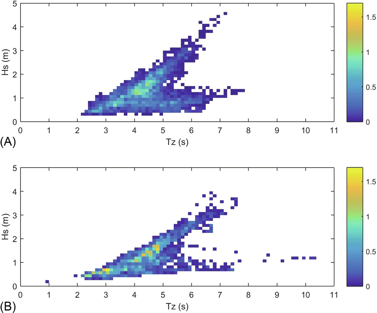
The model was validated against a half-hourly wave buoy time series archived by the Marine Institute in Ireland. The validation was performed from January 1, 2014 to March 31, 2014 (3 months) for both significant wave height (Hs) and zero upcrossing wave period (Tz).
Time series of observed and simulated variables are shown in Fig. 8.19. The model has clearly captured the temporal variability of the wave climate, but there are a few instances (e.g. beginning of January and February) when the model has under-estimated Hs by almost a metre. The scatter plots (Fig. 8.20) show qualitatively that there is very good agreement with Hs, and more scatter in Tz—this is a fairly typical trend in wave model simulations. The r2 value for Hs is 0.893, and the corresponding value for Tz is 0.417. The RMSE for Hs is 0.213 m (0.883 s for Tz), and S.I. for Hs is 18.2% (20.3% for Tz). Finally, bias is excellent, almost suspiciously so, for both Hs (0.0016 m) and Tz (0.035 s).


A final way of assessing model performance is to compare observed and modelled joint probability distributions between Tz and Hs (Fig. 8.21). Although this comparison is qualitative, it shows the success of the model in capturing both local and swell components of the wave climate.
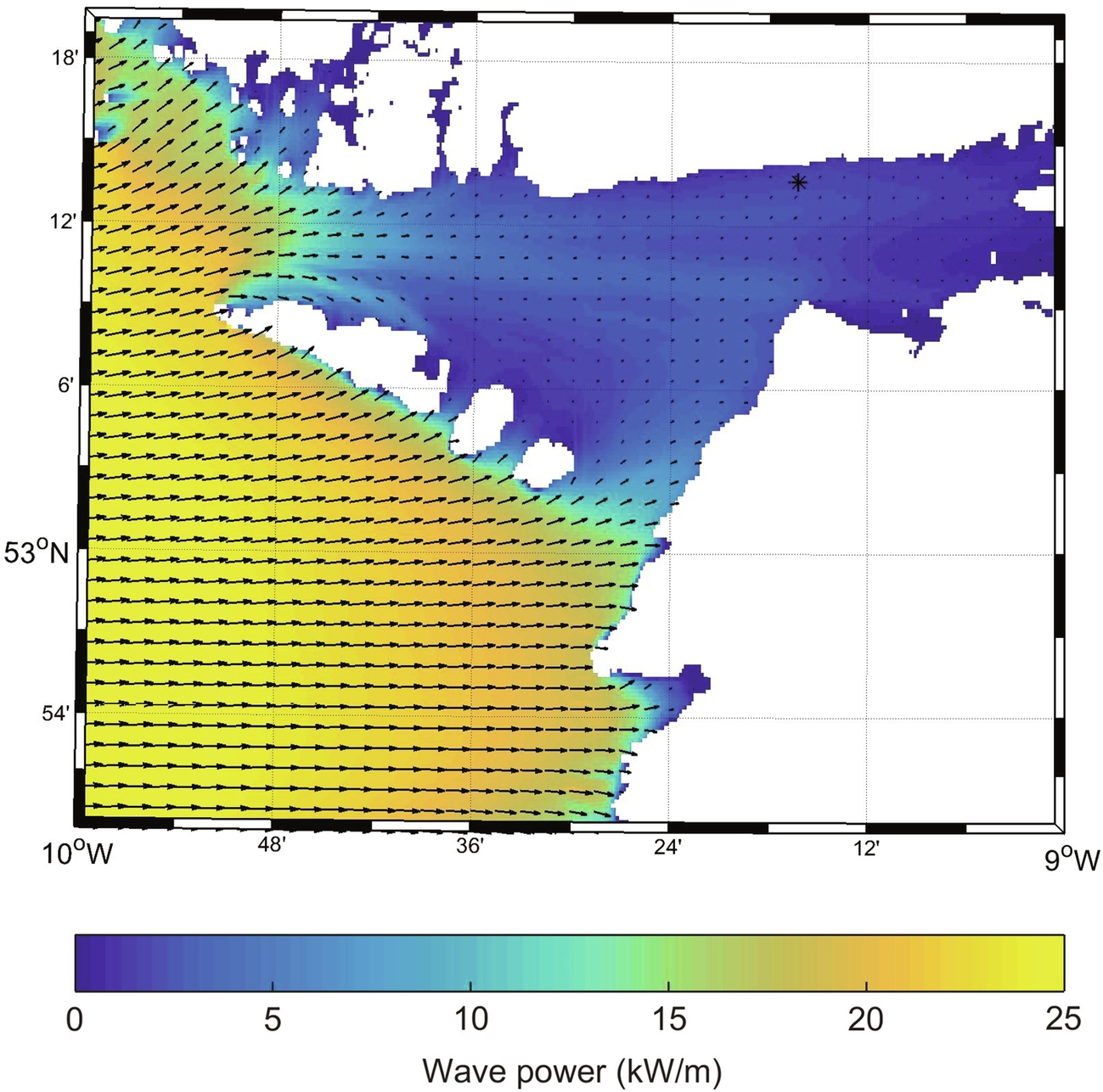
Results
The 2014 annual mean simulated wave power distribution demonstrates clearly how Galway Bay is sheltered from the North Atlantic (Fig. 8.22). The wave direction further offshore is predominantly westerly, but waves are refracted as they propagate into Galway Bay. One important consideration for a model, which includes complex topography at this scale (e.g. the Aran Islands), is choice of grid resolution. The resolution selected for this simulation (1/400 × 1/400 degrees) was appropriate for running an annual simulation in ∼48 h using 96 processors of a supercomputer. This resolution seems suitable for this duration of simulation, for example, the validation was successful, and the wave energy propagating between the Aran Islands appears to have been captured well (Fig. 8.22). However, for more detailed studies of shorter duration (e.g. storm) events, a higher-resolution simulation may be more appropriate; but at increased computational cost, since a higher grid resolution would require a smaller model time step (see Section 8.1.4).
8.9.2 Tidal Model of Orkney (Scotland)
Orkney is an archipelago in the north of Scotland, separated from the Scottish mainland by the 12 km width of the Pentland Firth. Orkney is comprised of around 70 islands, separated by a series of bays and energetic tidal channels (Fig. 8.23). Orkney is mesotidal; however, tidal waves in the region, dominated by the principal semidiurnal lunar (M2) and solar (S2) constituents, take around two-and-a-half hours to propagate around Orkney from the western to the eastern approaches of the Pentland Firth (Fig. 8.24), leading to a considerable phase lag across Orkney. This phase lag results in a strong pressure gradient across Orkney, driving very strong tidal flows through the Pentland Firth and along the Firths of Orkney. For example, the M2 phase lag between the Atlantic approach of Westray Firth and the North Sea approach of the connecting Stronsay Firth (Fig. 8.23) is around 65 degrees, that is 2.25 h,6 and the resulting flow is channelled through constrictions, which narrow to around 5 km, with water depths in the range 25–50 m.
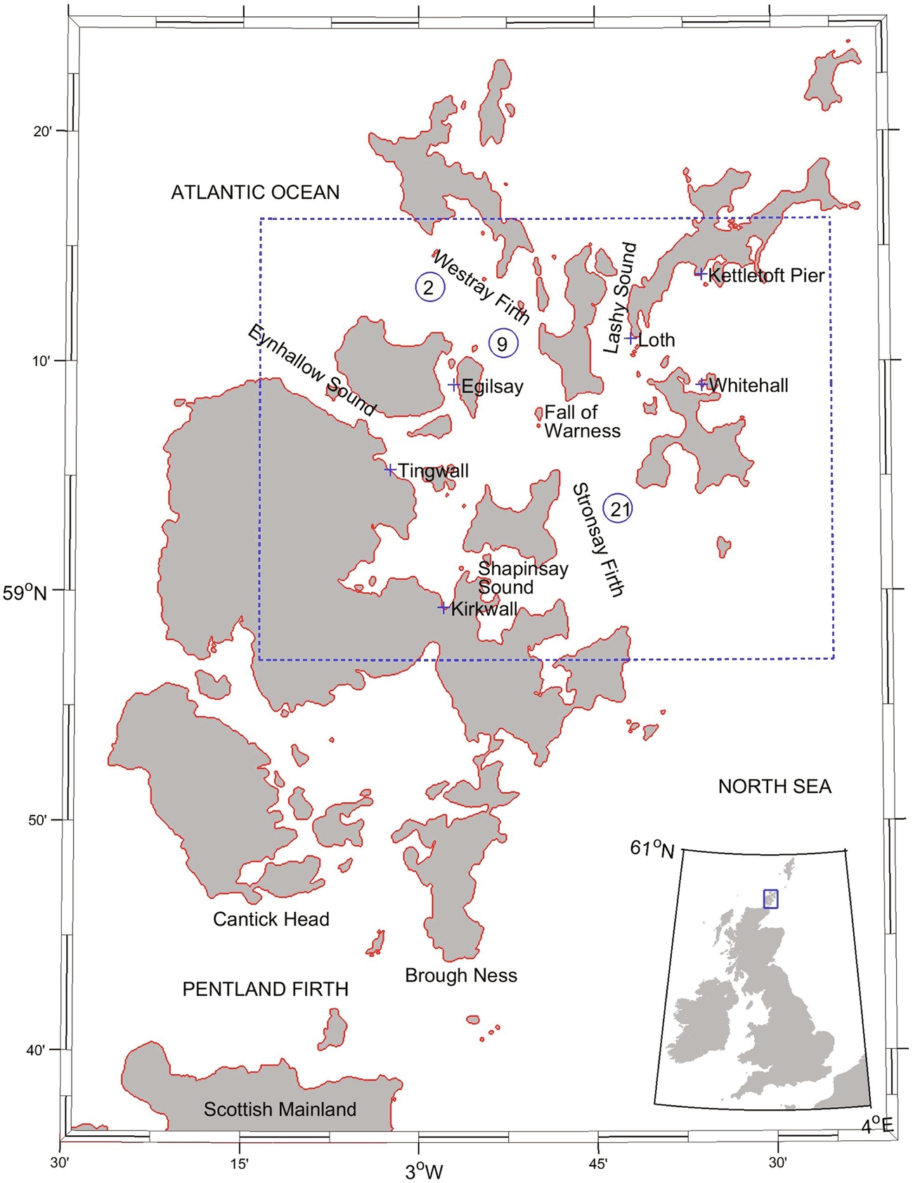

The tidal currents flowing through the interisland channels of Orkney exceed 3m/s in many regions [27], in conjunction with water depths in the range 25–50 m, suitable for the deployment of TEC devices. The marine renewable energy potential of Orkney has been recognized by the formation in 2003 of the European Marine Energy Centre (EMEC), which provides a wave test site to the west of Orkney, and a tidal test site in the Fall of Warness, situated where Westray Firth joins Stronsay Firth (Fig. 8.23).
The original aim of this model study was to investigate the role of tidal asymmetry on net power output (Section 3.10). However, the case study is presented here to demonstrate the setup of a 3D tidal model, and typical model outputs.
Model Setup
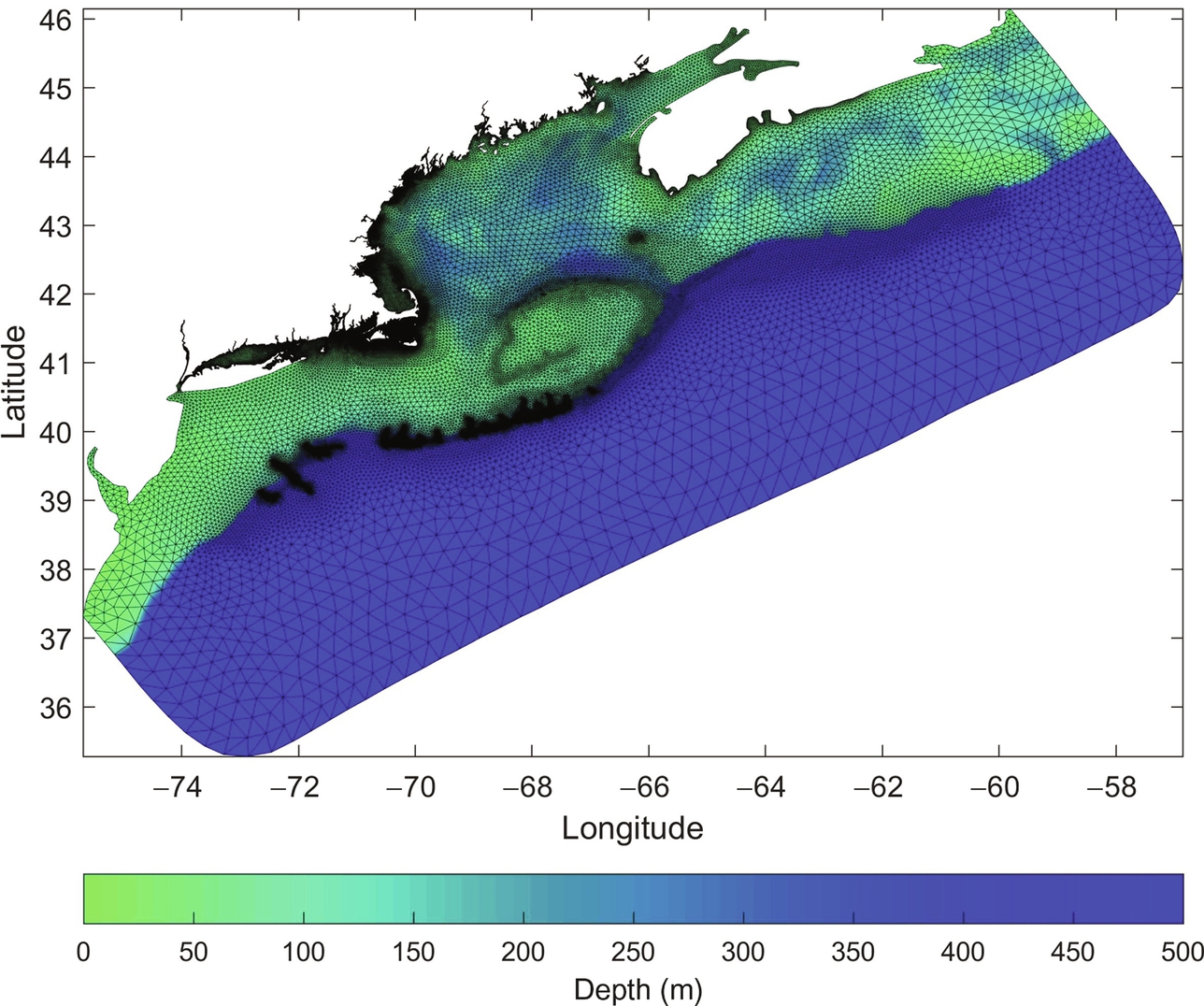
To provide boundary conditions to the high-resolution Orkney model, it was necessary to first run a north of Scotland regional model at coarser resolution. The regional model extended from 4degrees 30′W to 0degrees 30′W, and from 58degrees 18′N to 60degrees 03′N, encompassing the Pentland Firth, Orkney, and part of Shetland (Fig. 8.24). The regional model had a horizontal grid spacing of 1/120 × 1/228 degrees (approximately 500 × 500m), and was forced at the boundaries by FES2012 (1/16 degrees resolution) currents and elevations for the M2 and S2 constituents [28]. Bathymetry for the regional model was interpolated from 1/120 degrees GEBCO data. The regional model was run with 10 equally distributed vertical (sigma) levels for a period of 15 days, and tidal analysis of the elevations and depth-averaged velocities used to generate astronomical boundary forcing for the inner nested high-resolution Orkney model.
The high-resolution Orkney model extended from 3degrees 13.5′W to 2degrees 25′W and from 58degrees 57′N to 59degrees 16′N at a grid resolution of 1/750 × 1/1451degrees (approximately 75 × 75m) (the dashed box shown in Fig. 8.23). Bathymetry was interpolated from relatively high-resolution (approximately 200 m) gridded multibeam data provided by St. Andrew’s University. The model domain encompasses the principal high tidal flow regions of Orkney, including Westray Firth and Stronsay Firth, and the EMEC tidal test site at the Fall of Warness. The model configuration used the GLS turbulence model, tuned to represent the k-ε model, and included horizontal harmonic mixing to provide subgrid scale dissipation of momentum [29], and quadratic bottom friction, with a drag coefficient CD = 0.003. This value for the drag coefficient is consistent with previous ROMS studies which simulate the flow through energetic tidal channels, and these studies have demonstrated that the ROMS model is not particularly sensitive to the value of CD [30, 31]. The model was again run with 10 vertical levels for a period of 15 days.
Results
The peak depth-averaged tidal currents and the corresponding peak velocity vectors are shown in Fig. 8.25. Clearly, tidal flow is strongest at the constrictions of narrow channels (e.g. Lashy Sound, Eynhallow Sound, and, in particular, the Fall of Warness—see Fig. 8.23 for locations). The peak current speed reaches 3.7m/s in Lashy Sound and the Fall of Warness, and because the model was forced with the two principal semidiurnal tidal constituents, M2 and S2, these represent peak spring tidal currents. The peak velocity vectors also provide a qualitative overview of the tidal asymmetry [32], and the tidal flow appears to be largely ebb-dominant (peak currents directed northwest) in Westray Firth, and flood-dominant (peak currents directed southeast) in Stronsay Firth.7 Where these two Firths join (i.e. in the vicinity of the Fall of Warness), the circulation is further complicated by the presence of strong residual eddies with length scales of around 4–5 km [33]. However, the tidal currents in this region appear to be more symmetrical, and divergence of the peak velocity vectors indicates that this is a bed-load parting zone [32]. The bathymetric/topographic restriction of the Fall of Warness impedes the flow along the channel, which is driven by the tidal pressure gradient. This impedance results in an acceleration of the flow downstream of the restriction. This leads to a divergence of the residual flow centred on the Fall of Warness, which is further complicated by variability in bathymetry and geometry along and across the channel (Fig. 8.25).

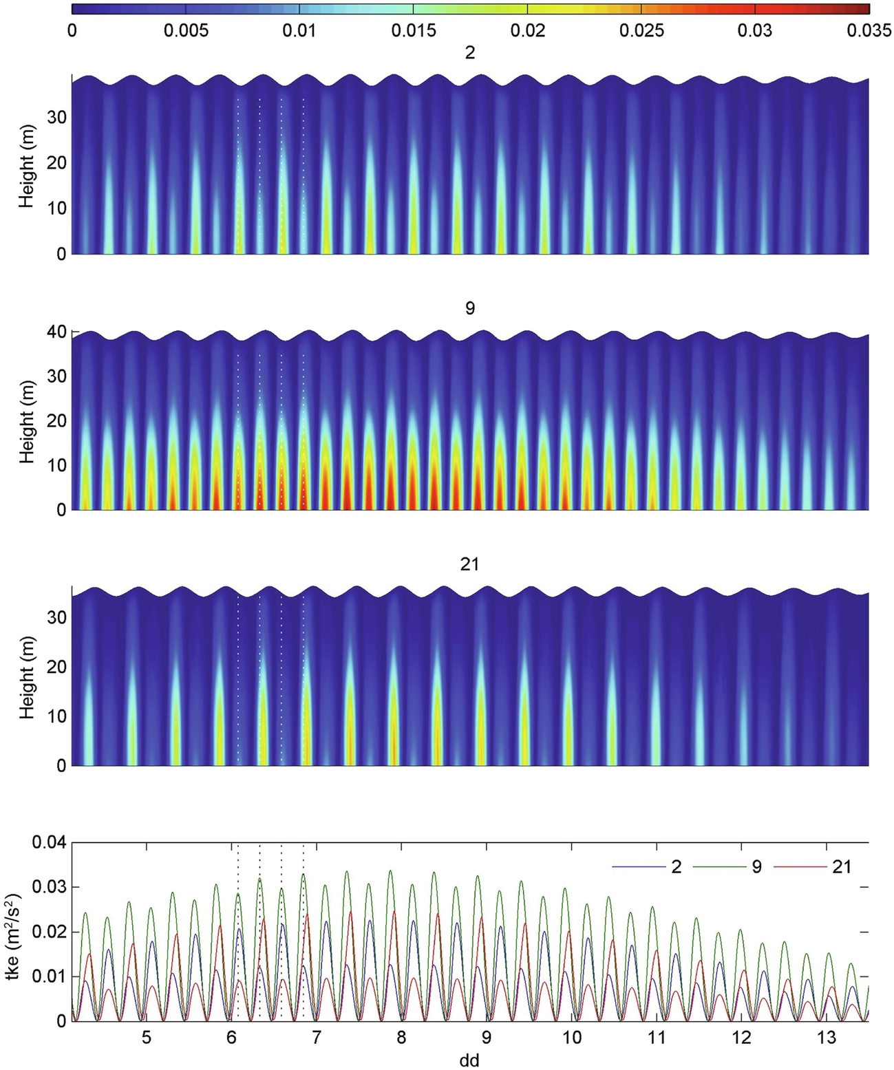
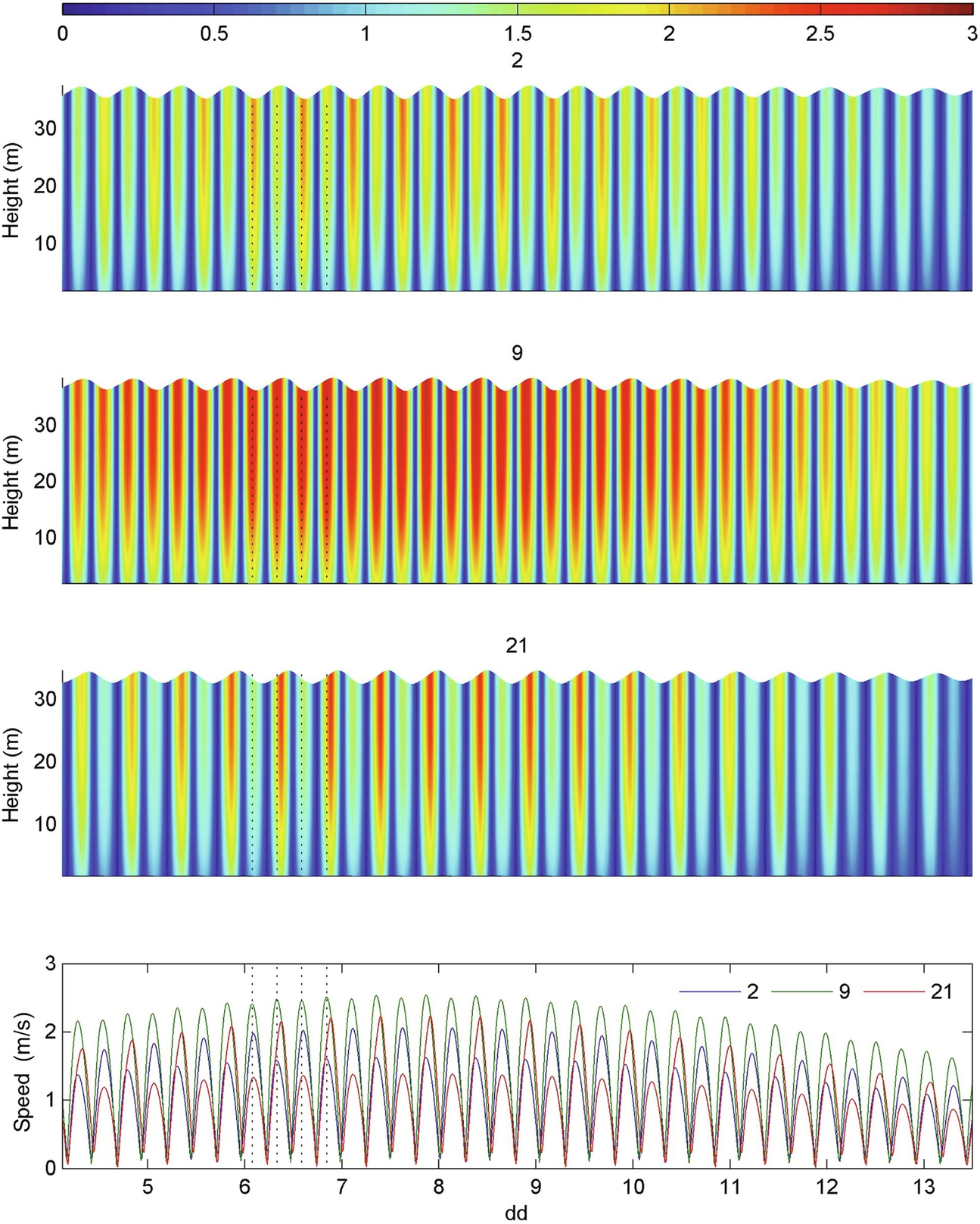
The advantage of a 3D tidal model, compared with a depth-averaged 2D model, is that the vertical distribution of variables in the water column is calculated directly, rather than parameterized. Here, we show detailed results for velocity and turbulence properties for all depths in the water column at three locations which exhibit varying degrees of asymmetry: site 2 (ebb-dominant), site 9 (symmetrical), and site 21 (flood-dominant) (Fig. 8.23).
Velocity time series for the three selected locations are plotted in Fig. 8.26. Above the boundary layer, the asymmetry for sites 2 and 21 is evident at all depths in the water column, and is more pronounced during spring tides. Therefore, for all practical scenarios of energy extraction, that is device hub placed at some height in the water column that is above the near-bed boundary layer, strong velocity asymmetry will translate into an even stronger asymmetry in power output (because power is related to velocity cubed). Such asymmetry in the flow field is clearly undesirable from an electricity generation perspective, and so symmetrical sites (such as site 9) are more attractive for commercial development.
Turbulent kinetic energy (k) per unit mass is defined as
k is plotted at three contrasting locations (Fig. 8.27). The corresponding plot for the rate of dissipation (ϵ) of k is shown in Fig. 8.28, defined as
where P is the rate of production. By comparing these turbulence metrics with the velocity time series (Fig. 8.26), it is clear that even a relatively modest asymmetry in velocity can translate into a large asymmetry in turbulence properties. Although sites 2 and 21 have the strongest asymmetry, this point is made clearer by considering the velocity time series at site 9 (Fig. 8.26) (an almost symmetrical site). This almost indiscernible asymmetry in the velocity time series manifests itself as a strong asymmetry in TKE (Fig. 8.27). The production of turbulent kinetic energy is generally proportional to the magnitude of the velocity gradient  . For a specific velocity distribution (e.g. a logarithmic distribution), this gradient will be proportional to the current strength. Therefore, we expect magnified turbulence asymmetry due to asymmetry in the current strength.