
Optimization
Abstract
To make the best use of an ocean renewable energy resource, for example, to maximize electricity generation whilst minimizing environmental impacts, it is necessary to perform optimization. Optimization theory has wide-ranging applications, but here we consider applications to offshore wind, tidal energy, and wave energy. Many intraarray optimization topics are common across the majority of ocean renewable energy resources, for example, optimizing device spacing and minimizing variability. We also consider interarray optimization within the context of tidal energy plants—a predictable resource with strong potential for phasing of power stations along a tidal wave, hence minimizing variability in aggregated power output. Finally, we introduce tools available for optimizing wind farms (HOMER) and tidal energy arrays (OpenTidalFarm).
Keywords
Optimization; Objective function; Micro-siting; Intraarray optimization; Wake effect; Device spacing; Park effect; HOMER
To make the best use of an ocean renewable energy resource, for example, to maximize electricity generation whilst minimizing environmental impacts, it is necessary to perform optimization. Optimization theory has wide-ranging applications, but here we consider applications to offshore wind, tidal energy, and wave energy. Many intraarray optimization topics are common across the majority of ocean renewable energy resources, for example, optimizing device spacing and minimizing variability. We also consider interarray optimization within the context of tidal energy plants—a predictable resource with strong potential for phasing of power stations along a tidal wave, hence minimizing variability in aggregated power output. Finally, we introduce tools available for optimizing wind farms (HOMER) and tidal energy arrays (OpenTidalFarm).
9.1 Introduction to Optimization Theory
Optimization is closely related to decision making; hence, we face many optimization problems in our daily life as an individual, company, organization, or government. When faced with several alternatives, we are always interested in the best alternative or decision. For instance, if you are planning a trip, you can choose amongst several alternative forms of transport, including flights, trains, rental cars, or bus. The best mode of transport would depend on your criteria, which is technically called the objective function. If minimizing the cost is the criteria, the best option may be transport by bus. If the objective is to minimize travel time, flights might be the best option. Any optimization problem needs an objective function. Usually, the objective function will be either minimized or maximized. Depending on the application, other names such as cost function (minimize in economy), profit function (maximize in marketing), fitness (maximize in genetic programming through natural selection), energy function (minimize in physics), or error (minimize in numerical modelling) are used. As an ocean science example, model parameter estimation (in calibration, inverse modelling, or data assimilation) is an optimization problem. Given a set of observed data, the best model parameters (e.g. bottom drag coefficient, wind drag coefficient, boundary conditions, etc.) are selected such that the error between model simulations and observations is minimized.
The objective function of an optimization problem depends on the independent variables, which can also be called decision or control variables. Independent variables in the ocean model parameterization example are physical properties of the ocean, such as bottom and surface drag coefficients. The objective function should be sensitive to independent variables. In some complex problems, a sensitivity analysis is performed to eliminate parameters or variables that do not affect the objective function. Independent variables can be discrete or continuous. For example, finding the optimum number of blades for a wind turbine is a discrete optimization problem; whereas finding the optimum distance between two wind turbines is a continuous optimization problem. Optimization problems are mostly formulated as deterministic problems, in which independent variables and objective function(s) are treated deterministically. In contrast, in stochastic optimization problems, due to uncertainties, random variables are used to formulate the problem. The expected value of the objective function is either maximized or minimized in such problems. For instance, optimizing the operational cost of a renewable energy micro-grid can be treated stochastically due to uncertainties in supply of energy (i.e. intermittency of the resource [1]).
An optimization problem may be subjected to constraints. Referring to our earlier example of finding the best mode of transport for a journey, assume that minimizing the time is the objective function, but you may not exceed a certain budget for the transportation cost. In that case, the problem becomes more complicated. For instance, direct flights may exceed your budget. Technically, any alternative that does not satisfy constraints is not feasible, or out of the feasible region or search space. The best solution to the transportation problem may be found by comparing indirect flights and trains that do not exceed your budget. In the model parameterization example, an acceptable/feasible range for each parameter is applied as a constraint. For instance, bottom friction cannot be a negative number.
An optimization problem may have one, two, or multiple objective functions that are conflicting. For instance, assume that you are trying to determine the best type of energy system for an off-grid island community. Your first objective function is to minimize the cost; your second objective function can be minimizing pollution (i.e. emission of pollutants such as CO2). These objective functions are conflicting; the best solution may not be the least expensive or the cleanest type of energy for the island. The majority of real life decision-making problems, including renewable energy systems, have multiple objective functions, and are subjected to various constraints.
Optimization problems are either static or dynamic. In dynamic optimization problems, the parameters of the problem change with time. Finding the best trajectory of an aeroplane over a fixed range (minimum fuel cost and minimum travel time) is a dynamic optimization problem, because the environmental conditions that affect the fuel consumption and travel time of the aircraft (e.g. wind) change with time. In energy-related projects, several variables, such as the price of energy, demand, and interest rates, vary with time; therefore, many renewable energy optimization problems are dynamic in nature.
Simple optimization problems were first introduced in calculus: finding the maximum or minimum of a function. More realistic applications of optimization theory were introduced in World War II in order to reduce the cost of an army and maximize loss to the enemy. Since then, and mainly due to advances in computing power, numerous methods/algorithms have emerged to solve optimization problems, and have been applied across various disciplines. These methods can generally be categorized as linear programming, nonlinear programming, iterative methods, and metaheuristic techniques. In linear programming problems, the objective function and constraints are linear—as opposed to nonlinear programming. Metaheuristic approaches are the most recent suite of optimization techniques, and are mainly based on artificial intelligence and machine learning. Evolutionary algorithms, genetic algorithm, and particle swarm optimization are popular metaheuristic approaches.
Solution techniques for optimization problems can be classified as trajectory- and population-based. In the former method, a single solution is used to search for the optimum. The optimum solution is also a single-optimized solution at the end of the optimization process. Classical iterative schemes such as Newton’s method fall into this category. In population-based techniques, a population of solutions are used that evolve through each iteration of the optimization. In general, a set of optimum solutions are provided at the end. An example is genetic algorithms that provide a set of solutions that have the best fitness (e.g. above an acceptable value). For decision-making applications, population-based techniques are more attractive, because they give decision makers a chance to select amongst a list of optimum solutions.
There are several excellent books describing various classical and modern optimization techniques (e.g. [2, 3]). Here, an overview of the basic concepts, some examples, and tools to optimize ocean renewable energy projects are introduced.
9.1.1 Mathematical Formulation of an Optimization Problem
An optimization problem can be mathematically formulated as follows:

in which f is the objective (cost, fitness, etc.) function, xi are independent or decision variables, and Ω represents the feasible region or search space. As mentioned before, we could also maximize the objective function (e.g. fitness). Any maximization problem can simply be converted into a minimization problem by multiplying the objective function by − 1. The feasible, or search space, is controlled by the constraints of the problem.
For instance, assume that the location of four wind turbines in an offshore wind farm needs to be optimized. For this problem, the objective function can be defined as electricity production. The decision variables are the geographical coordinates of these four turbines: (x1, y1;x2, y2;x3, y3;x4, y4). The production of electricity in this small array depends on the decision variables, because both the available wind energy resource, and the wake of each turbine (that may adversely affect power output for another turbine) are controlled by turbine locations. The feasible space or constraints can be defined as the leased area of the farm, because none of these turbines can be installed outside the allocated area. This can be mathematically formulated as a ≤ xi ≤ b and c ≤ yi ≤ d, where a, b, c, and d define the geographical boundaries of this problem. This type of constraint is called inequality constraint. Equality constraints can also be applied. For the simple wind farm example, assume that, for aesthetic reasons, we want to install all four turbines in a straight line. Therefore, the geographical locations of all turbines must satisfy the equation of a line (i.e. mxi + nyi + q = 0). In general, an optimization problem can be formulated as
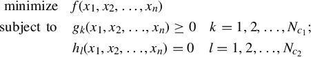
where gk and hk represent inequality and equality constraints of the problem. ![]() and
and ![]() are the number of inequality and quality constraints, respectively; an optimization problem can have several inequality or equality constraints. It should be noted that applying too many constraints can make an optimization problem infeasible (e.g. if constraints are mutually contradictory), and so result in no solution.
are the number of inequality and quality constraints, respectively; an optimization problem can have several inequality or equality constraints. It should be noted that applying too many constraints can make an optimization problem infeasible (e.g. if constraints are mutually contradictory), and so result in no solution.
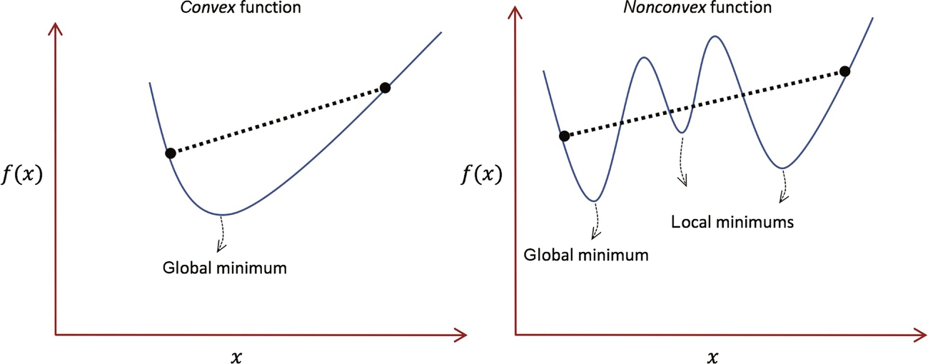
The optimum solution of a problem can be local or global. Referring to Fig. 9.1, a function can have several minimums/optimums. The local optimum is a solution that is better than the neighbouring points, but not necessarily the best solution across the search space. If the objective function is convex (left plot in Fig. 9.1), there is only one minimum or optimal solution. By definition, a function is convex if the line segment connecting two points on the function always lies above it. This is not the case for the right-hand plot in Fig. 9.1, which is nonconvex. This definition can be generalized as a function with several variables. Although the majority of real life optimization problems are nonconvex, classical, simple optimization techniques can quickly find local optimums. Global optimization techniques are more complicated and, accordingly, more computationally expensive.
9.1.2 Search Methods and Optimization Algorithms
To briefly explain how an optimization algorithm works, the basic concepts of search techniques are explained here. An optimization technique searches for a point that minimizes the objective function. Many mathematical techniques are iterative. They start from an arbitrary initial point in the search space and update that point during each iteration:
in which α is the step size, and g is the step direction. During each iteration, the decision variable vector is updated using Eq. (9.3); step size and step direction are computed based on the optimization algorithm (e.g. maximum gradient). Fig. 9.2 shows a 2D schematic of an optimization that starts at point x1 and moves iteratively towards the optimum point.
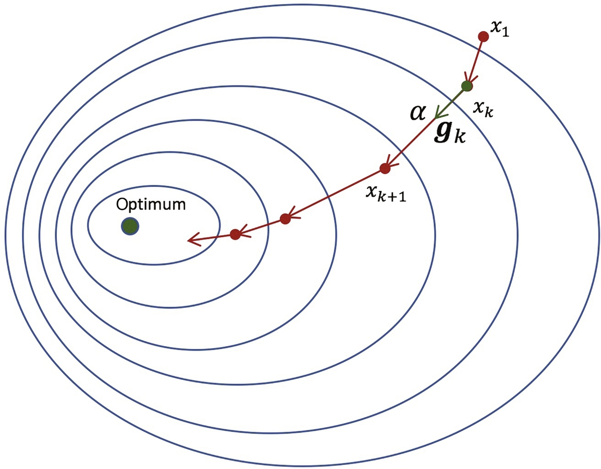
A simple analogy to optimization is climbing towards the summit of a mountain (maximum elevation). Here, the objective function is elevation, and latitude and longitude are the decision variables. Assume that a helicopter leaves you at a random location on the mountain. Based on the best local information, you move towards a direction for a specific distance (step size), and then you change your direction. The distance that you move in each direction is not necessarily the same: the step size can also vary within each iteration. An obvious direction is going up, and in particular in the steepest ascent direction. The steepest ascent is mathematically the direction of the gradient, which can be written as
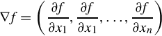
and the method of steepest ascent becomes
This method almost guarantees that you reach a summit that is closest to your initial location but, as you can imagine, it does not guarantee that you will reach the highest summit of a mountain range. Many classical optimization techniques are based on gradient. The method of steepest ascent (or descent in minimization) is not very effective, especially near the solution. Referring to Fig. 9.1, it is clear that the gradient of the function (slope of the tangent) near the local and global minimums approaches zero. This causes some issues for methods that only use gradient for the direction. Other techniques are called conjugate gradient methods that use second derivatives (Hessian matrix) as well as first derivative (gradient) for direction.
9.2 Intraarray Optimization
Although understanding the natural (undisturbed) resource, and the operation of single devices, is essential, it is only when devices are installed in arrays that significant levels of electricity generation can be achieved. In this section, we discuss how devices within such arrays can be optimized for wind, tidal stream, and wave energy conversion.
9.2.1 Micro-Siting of Offshore Wind Farms
Referring to Section 4.4, marine spatial planning is the standard procedure used to find suitable and potential sites for the development of offshore wind farms in a region. Marine spatial planners, after a comprehensive study of technical, economic, environmental, sociopolitical, legal, and regulatory aspects, recommend areas that have minimum conflicts with other users of the ocean, in addition to a feasible energy resource. Macro-siting is the selection of a location for a wind farm within these recommended areas. Macro-siting can also be treated as an optimization problem, which is not discussed here.
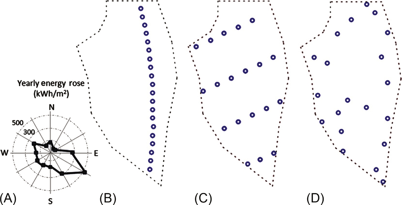
After selection of a location/plot for an offshore wind farm, the best layout of turbines within a farm needs to be determined. The layout, in general, consists of the number of wind turbines, and the size and geographical location of each turbine. In many cases, the maximum investment, or the capacity of a farm, is decided in the first steps of a study as a constraint; therefore, if the size of the individual turbines is also established, the optimization problem reduces to finding the best/optimum geographical location for each turbine. This is referred to as micro-siting of offshore wind farms. Fig. 9.3 shows an example of wind farm optimization that can lead to around 5% increase in annual energy production (AEP; [4]).
Wake Effect
The layout of wind turbines in a wind farm affects AEP of the array. As we discussed in Chapter 4, wind has spatial variability; therefore, if the farm is large enough, in some places wind energy is higher than other places. If variability of the available resource was the only reason, we could just locate wind turbines in places that have the highest energy. A more complicated issue is the interaction of a wind turbine with neighbouring turbines. Fig. 9.4 shows how turbines can be located in the wake of each other under particular wind conditions. The wind speed in the wake of a turbine is significantly lower than the undisturbed wind speed (in the absence of the upwind turbine). This reduction of speed adversely affects total AEP. It is possible to place turbines very far from each other to avoid wake effects, but this can lead increased cost of cabling, electrical connections between turbines, maintenance cost, and a larger leased area. Therefore, finding the optimum layout is an optimization problem.

Estimating the reduction of wind speed in the wake of a turbine can be achieved by simplified methods, based on the distance of the turbines, hub height, and radius of turbines (e.g. [5, 6]), or wakes can be more accurately simulated using CFD codes and high performance computing (e.g. [7, 8]).
Decision Variables
In micro-siting of offshore wind farms, the layout of the farm, which consists of several variables, needs to be optimized. The simplest case is when the number and the capacity of turbines are given, in which the locations of the turbines are the decision variables. More complicated cases involve more decision variables, such as the number, size, type, and hub-heights of turbines, in addition to the locations of the wind turbines.
Objective Functions
As mentioned before, a renewable energy system can be optimized by a single or multiple objective functions. The simplest objective function is AEP (maximize). This objective function does not take into account the cost associated with AEP, which is a major factor in the decision-making process. Referring to the concept of levelized cost of energy (LCOE) introduced in Chapter 1, the ratio of the cost of energy to electricity production can be minimized, which is a more practical objective function. This objective function takes into account the increased cost of electrical cables and other elements of the farm when turbine spacing is increased:
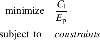
where Ct can be chosen as the total cost of the project, and Ep is the total energy production during the lifetime of the project. Alternatively, the investment cost divided by AEP can be minimized, which does not take into account the interest rate, operation and maintenance cost, and the time value of money.
Constraints
Micro-siting is subject to several constraints. The most common constraint is the available area/plot for the farm (i.e. all turbines should be located inside the array). The minimum distance between turbines can also be a constraint due to technical issues or standards/regulations. Another constraint is the maximum available investment. Although a large project can produce reasonable and lower LCOE, the resources for financing a project are usually limited. The layout of a wind farm may be subjected to some constraints to reduce the visual impact or improve aesthetic design (e.g. Fig. 9.3B). Finally, forbidden areas in a farm can limit the search space. These areas may be excluded due to foundation issues, dedicated to electrical cable routes, etc.
Solution Techniques
Due to the complexity of the objective function and constraints of the wind farm optimization problem, classical optimization techniques that are often more suited to convex and continuous problems are less popular. Therefore, metaheuristic methods are more effective and common in this area. Metaheuristic approaches provide satisfactory solutions, but they do not necessarily find the theoretical optimum. Genetic algorithm, particle swarm optimization, the greedy algorithm, evolutionary algorithm, and ant colony are metaheuristic approaches applied in this area [5, 9].
9.2.2 TEC Array Optimization
Interdevice Spacing
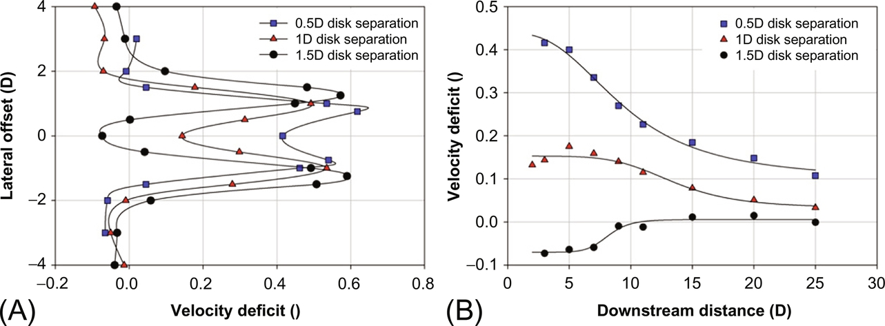
The 2009 EMEC guide the assessment of tidal energy resources [10] recommends that the lateral spacing between devices (the distance between axes) should be two-and-a-half times the rotor diameter (2.5D), and the downstream spacing should be 10D—both based on the assumption of horizontal axis turbines. Further, the EMEC guide states that devices should be positioned in an alternating downstream (i.e. staggered) arrangement (Fig. 9.5). Although the exact details of device spacings is device-specific and can be debated (and indeed no justification is given for the values 2.5D and 10D, although we can assume that such guidance has propagated through from the wind industry), the reasoning behind the spacings is introduced here. Each tidal stream device will generate a wake—a relatively narrow turbulent region downstream of the device where the velocity is below ambient. Clearly, placement of a subsequent device within this wake zone would lead to suboptimal device performance (e.g. increased turbulence), and so not exploiting the resource to its full potential (because the velocity in this region is below ambient). Therefore, the guidance of spacing devices 10D in the longitudinal direction is designed to minimize the wake effect. In addition, by staggering the devices, this will further prevent a device positioned downstream of another device from operating in its wake (Fig. 9.5). Myers and Bahaj [11] investigated the impact of lateral device spacing. They found that for very close lateral turbine spacings (0.5D measured between the innermost edges of the actuator disks, which is equivalent to 1.5D in the EMEC guidelines; based on flume experiments where the turbine rotors were represented by porous disks), the individual wakes generated by each of two devices merged by around 4D downstream. At increased lateral spacings (1.5D), a region of around 1D width accelerated flow between the two disks resulted, indicated by a negative velocity deficit1 in Fig. 9.6. Therefore, for a final experiment, Myers and Bahaj [11] placed a third ‘turbine’ 3D downstream of the first row of disks in an attempt to exploit this region of accelerated flow. Although they did not perceive any significant negative changes to the efficiency of this third device, they found that the far wake region of the array had a relatively high velocity deficit due to the combined wakes, and so a third row of devices would need to be installed at a considerably increased longitudinal spacing to enable interception of flow speeds comparable to the first row. Of course, flume experiments such as this are unidirectional, and so bidirectional (tidal) flows will require further consideration, for example, the ‘first’ row during the flood phase of the tidal cycle will become the ‘last’ row during the ebb.

Apart from potentially making use of regions of accelerated flow to strategically site devices (as discussed above), it is clearly advantageous, from both economic and practical perspectives, to minimize lateral and longitudinal extents of tidal energy arrays. Many leased tidal energy sites are situated in relatively narrow straits, where the principal flow dimension is much greater than the lateral channel dimension. Therefore, due to physical and navigational constraints, a more compact lateral array configuration (and hence spacing) is desirable. Excessive longitudinal spacing will significantly increase subsea cable lengths (e.g. the range of 5D–15D longitudinal spacing to avoid wake effects equates to 100–300 m for a 20 m diameter turbine), but such potentially increased cabling costs would depend on the design of the subsea connections and cable route between the devices and the substation (e.g. [12]).
Blockage
The theoretical upper limit to power extraction by a wind turbine is constrained by the Betz limit (Cp = 0.59), where Cp is the rotor power coefficient (see Section 3.13.1). However, in wind energy conversion, the cross-sectional area (CSA) of the turbine is very small in comparison to the CSA of the wind resource. By contrast, when tidal turbines are placed in a tidal channel, the turbine blockage ratio2 increases, resulting in a theoretical Cp that can considerably exceed the Betz limit for array scales/configurations that are characterized by high blockage ratios [13]. However, the situation is complicated by the fact that by increasing the blockage ratio of a channel, there will be a corresponding reduction in the free-stream flow due to the increased drag resulting from tidal energy conversion. In other words, placing too many turbines in a tidal channel will merely block the flow.
To maximize turbine efficiency (i.e. the power available per turbine), tidal arrays should occupy the largest possible fraction of a channel’s CSA [14]. However, practical constraints, such as navigation and the passage of marine life, will require gaps between the turbines in an array. In such a scenario, energy is dissipated in the wakes, and so the turbines are less effective than if they were deployed in a fence that spans the entire channel3 [15].
An interesting extension of the work on simple tidal channels (e.g. [15]) is application to split channels [16]. Split channels are fairly common amongst tidal energy sites—for example, the Bay of Fundy, Puget Sound, and the Pentland Firth. How, for example, would large-scale tidal energy extraction in the Inner Sound influence the tidal energy resource within the Pentland Firth itself (Fig. 9.7)? In addition, for scenarios where there is a fairly equal channel division, devices could be strategically installed on one side of an island, leaving the opposite side clear for navigation [16]. Polagye and Malte [17] simulated a range of channel networks, including a split tidal channel (which they call a multiple-connected network). They found that transport in the impeded channel reduced, at maximum power, to around 50% of its magnitude compared with its undisturbed state. This is agreement with Cummins [18], who found, using an electric circuit analogue, that the transport in the impeded channel was reduced to 50–71%: a similar range to the much reported 58% calculated by Garrett and Cummins [19] for a single channel in the resistive limit. Polagye and Malte [17] found that maximum dissipation (Pmax) was 20% higher when extraction was evenly distributed between the two branches (Fig. 9.8), and that an even distribution minimizes far-field impacts. However, such an optimal arrangement may be neither desirable (e.g. it would preclude the dedicated navigational channel mentioned earlier) nor attainable (e.g. natural flow asymmetry between the two channel branches).

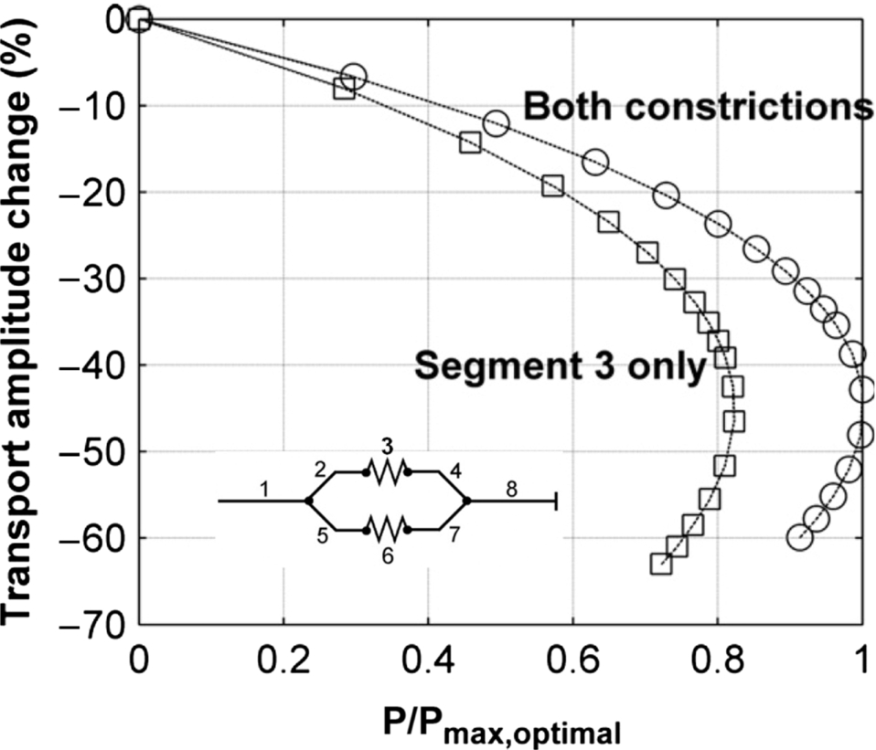
 denotes extraction only from segment 3 (upper branch). ○ denotes equal extraction from segments 3 and 6 (both branches). (Reproduced from B.L. Polagye, P.C. Malte, Far-field dynamics of tidal energy extraction in channel networks, Renew. Energy 36 (1) (2011) 222–234, with permission from Elsevier.)
9.2.3 WEC Array Optimization
Park Effect
Since a renewable energy converter absorbs energy from its surrounding environment, the total available resource is reduced for neighbouring energy converters [20]. For a wave energy converter (WEC) array, the ‘park effect’ Q can be represented as the ratio of the power of the full array (Ptot) to the sum of the power for each isolated WEC (Pisolated)

where N is the number of WECs in the array [21]. Although it is theoretically possible for some WEC array configurations to result in constructive wave interactions (i.e. Q > 1), in general Q < 1, and array designs tend to focus on limiting destructive interferences [20]. As the number of devices in a WEC array increases, the mean power per WEC reduces (Fig. 9.9B); but it is possible to minimize such destructive interferences through optimization of various parameters such as array geometry and device spacing.

Smoothing Power Fluctuations
Wave energy comes in pulses, and so is unsuitable for direct conversion and transmission to the electricity grid [22]. The addition of devices to an array reduces the variance in power (Fig. 9.9A); however, at the expense of reduced average power per WEC due to the park effect (Fig. 9.9B). In sea trials with WECs, Rahm et al. [22] found that there was an 80% reduction in the standard deviation of electrical power output from three WECs, compared with the standard deviation from a single WEC. Based on model simulations of a larger number of WECs [21], normalized variance of power ![]() (where variance V ar = σ2 and σ is the standard deviation) reduced from ∼0.9 to ∼0.4 for 4 to 64 WECs, respectively (Fig. 9.9A).
(where variance V ar = σ2 and σ is the standard deviation) reduced from ∼0.9 to ∼0.4 for 4 to 64 WECs, respectively (Fig. 9.9A).
Geometry of WEC Layout
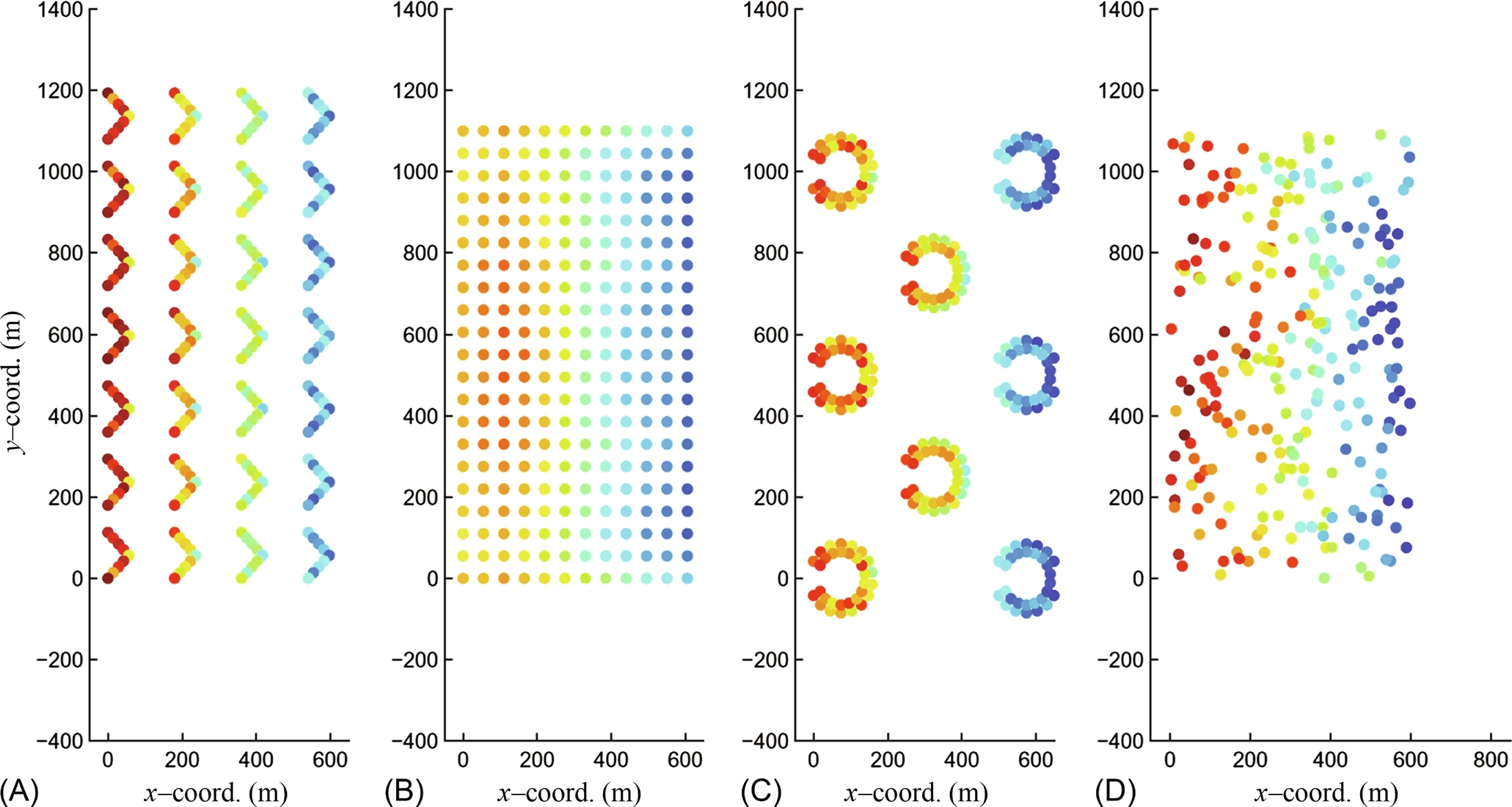
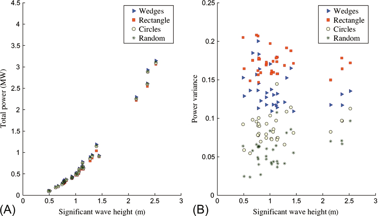
It is possible to further smooth power fluctuations through careful consideration of the geometric WEC layout [22, 23]. It has been shown that ‘global’ array layouts can increase power by 5% or reduce power by 30% [24]. Göteman et al. [25] simulated four global geometries, each with the same number of WECs (Fig. 9.10). Device spacings for the different configurations varied within the range 20–55 m, other than for the ‘random’ layout, where the minimal device spacing was set to 6 m. Because the incident waves propagate in the x-direction, clearly those devices at the rear of each array (increasing x coordinate) absorbed less power. However, it was not always the first row that absorbed the most power; for the rectangular configuration, it was the third row that absorbed most power, demonstrating a positive interference effect from the other WECs in the array. All four configurations resulted in similar energy absorption (Fig. 9.11A); however, power variance differed significantly between the four cases: ‘rectangular’ and ‘random’ layouts led to the highest and lowest variance, respectively (Fig. 9.11B). Engström et al. [26] investigated WEC array layouts that were only slightly randomized, that is, to represent uncertainty in mooring positions and temporal drift, again finding a reduction of variance in these more realistic ‘randomized’ layouts. This could be explained by considering regular WEC layouts that are aligned with the dominant wave direction (e.g. Fig. 9.10B). In this case, the electricity produced by all of the WECs distributed along the wave crest will generally be in phase for each WEC row. Staggering the devices slightly in the direction of wave propagation would introduce more phase diversity into the array, leading to more stable (less variable) aggregated power output. Minimizing the lateral dimension of the WEC array, and maximizing the longitudinal dimension, will have a similar effect, provided the longitudinal spacing is considered, in conjunction with the expected wavelengths. For example, a WEC array of 4 × 5 has lower variance if there are five rows along the direction of wave propagation, as compared to four [21].
Device Spacing
The spacing between individual devices within a WEC array has been shown to influence variance in power output. As summarized by Göteman et al. [21], a 3 × 3 square wave array covering an area of 400 m2 (10 m device spacing) has considerably lower variance than an array that covers 1600 m2 (20 m device spacing). A relatively closely spaced WEC array, provided the ‘park effect’ is minimized, will have the added advantage of lower cabling costs, that is similar to cabling issues associated with the longitudinal and lateral spacing of tidal energy devices (Section 9.2.2). In a further study of a 3 × 3 array of point absorbers, Göteman et al. [25] found a localized peak in power variance associated with 18 m device spacing. Although this exact value is unique to this particular device, it demonstrates that careful design is required to avoid nonoptimal device spacings.
Size of WECs in an Array
One final issue in WEC array optimization is the size of individual devices within an array. Consider Fig. 9.10, for example, where larger WEC devices would be more suited to the ‘front’ of the array, and smaller devices to the ‘rear’. Blending WEC sizes within an array can lead to higher power output for the array [21] and, it could be assumed, lead to more efficient use of each WEC within the array. Indeed, a concert of wave energy devices within a single array, each exploiting different parts of the wave energy spectrum, could be achieved, but only as a result of detailed knowledge of the wave climate, and extensive optimization.
9.3 Interarray Optimization
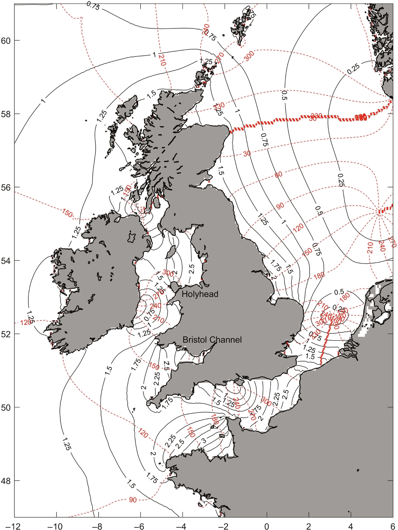
Examining the M2 (principal lunar semidiurnal) cotidal chart of the northwest European shelf seas (Fig. 9.12), Kelvin waves take a relatively long time to propagate along a coastline. For example, the southern part of the Irish Sea (around the Bristol Channel in Fig. 9.12) has a phase difference of around 3–4 h compared with the northern part of the Irish Sea (e.g. Holyhead). Because tides are predictable, it seems feasible that, with knowledge of the phase relationship between tidally energetic sites, we could strategically station a series of tidal power stations along a coastline, concurrently exploiting different parts of the same tidal wave, feeding the generated electricity into a unified electricity grid, and so reducing the variability that would result from a tidal power station operating in isolation.
9.3.1 Phasing of Tidal Stream Arrays
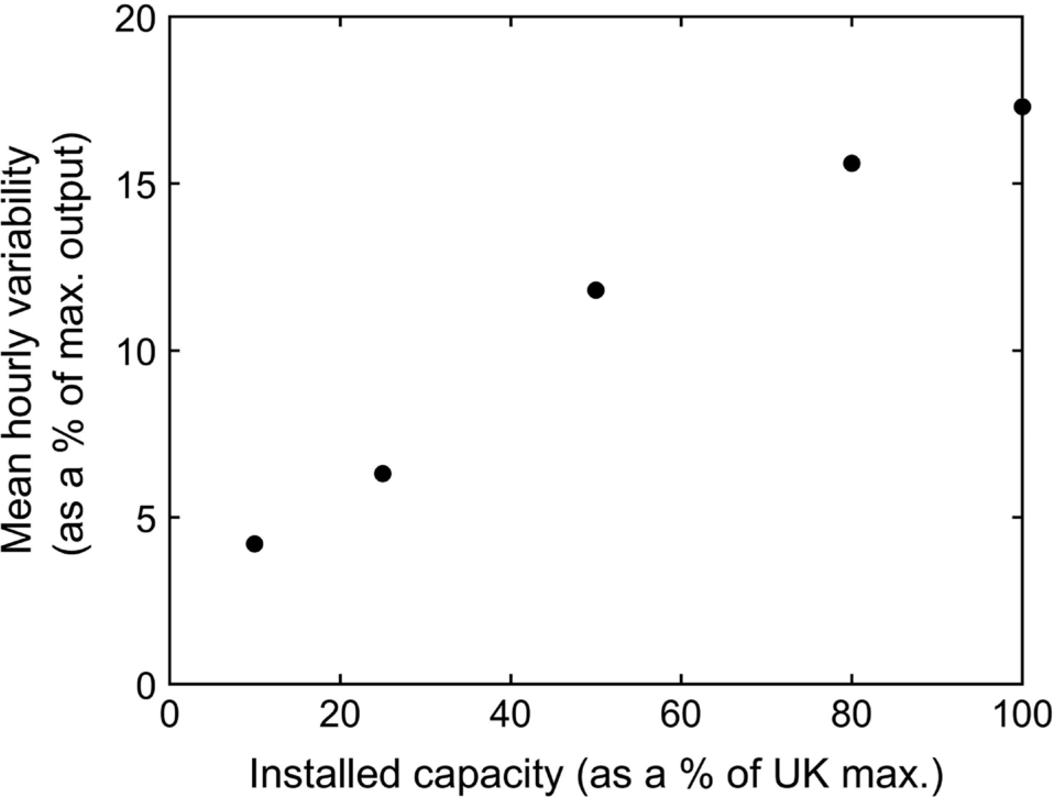
A 2005 study commissioned by The Carbon Trust [27] examined the patterns of energy availability from a range of tidal stream regions around the United Kingdom, with a focus on opportunities for diversification to reduce the variability of supply. The study is fairly comprehensive, but the results on optimizing variability can be summarized by reference to Fig. 9.13. In this figure, a range of development scenarios have been considered, from a relatively low level of development (10% of the UK tidal stream resource) up to an extreme scenario of 100% development. Within each of these development scenarios, optimization modelling was used to determine the contribution of each tidal stream site that resulted in the lowest average hourly variability (expressed as a percentage of maximum output). Development of 10% of the UK tidal stream resource across a range of sites would result in low variability. However, at larger scales of development, the synchronized output of larger sites (e.g. the Pentland Firth) dominates, increasing variability. For example, at 10% development, the Alderney Race (Channel Isles) accounts for 25% of all output compared with 10% for the Pentland Firth. However, at 100% development, the percentage contribution of the Alderney Race reduces to just 6%, whereas the Pentland Firth would account for 30% of the total output.
The issue of tidal phasing of tidal stream locations was revisited by Iyer et al. [28], who extended The Carbon Trust study [27] to include energetic sites in Wales: Anglesey (Skerries) and Ramsey Sound. Again, they concluded that there is insufficient diversity between the sites identified across the United Kingdom to be considered as a firm power source. In general, they found that the high-energy sites were in phase with one another, with the exception of Alderney Race in the Channel Isles. The problem was further investigated by Neill et al. [29, 30] who, rather than constraining their analysis to a limited number of locations, considered the UK tidal energy system as a whole. By doing so, they did not limit their analysis solely to high energy sites, but considered a diverse range of current magnitudes in the analysis. In addition to seeking sites with high energy, they penalized site selection where the combination of multiple sites led to a reduction in phase diversity. A summary of the findings of Neill et al. [30] is presented in Fig. 9.14. Because the high-energy tidal stream sites are generally in phase with one another, there is high variability in the resulting (aggregated) power—in agreement with previous studies [27, 28]. In contrast, there is considerably more phase diversity amongst less energetic sites. Therefore, an energy policy that seeks to minimize variability in the developed tidal stream resource would be advised to include lower-energy sites in the energy mix. Optimization, in this case the greedy algorithm with penalty function, led to a proposed road map for the evolution of a UK tidal stream industry (Fig. 9.15), with the key assumption that the Pentland Firth is the first region to host an array—an assumption that has now been proven to be valid with development of the MeyGen array. It is noted, in common with the Carbon Trust report [27], that at very high levels of tidal stream development, limitations on sea space would lead to an aggregated electricity signal that is dominated by relatively few high tidal stream locations, with a particular focus on the Pentland Firth. Incidentally, none of these studies included feedback between energy extraction and the resource—a topic that is covered in Chapter 10. In reality, at such large scales of exploitation, these feedback effects would be significant, and so there is a gap in knowledge of how best to optimize at interarray scale.

9.3.2 Phasing of Multiple Tidal Range Power Plants
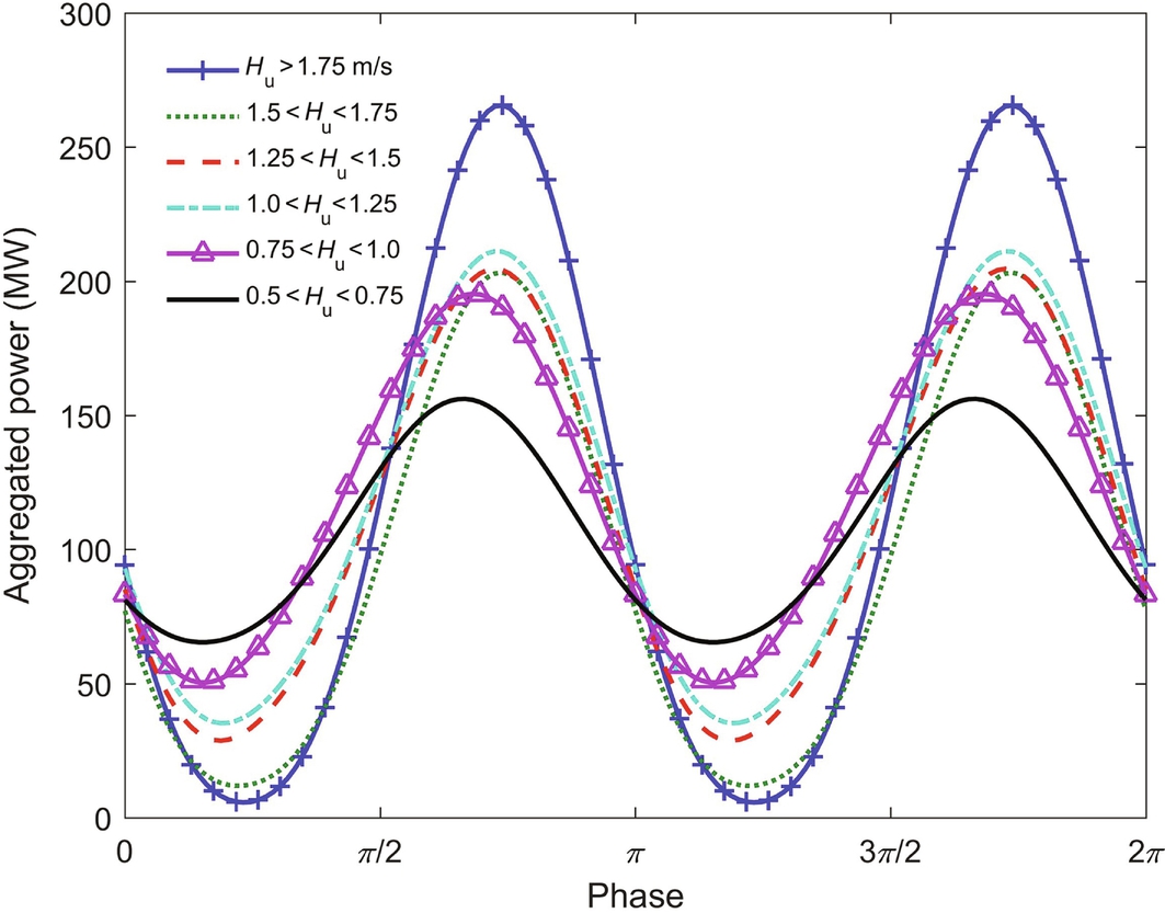
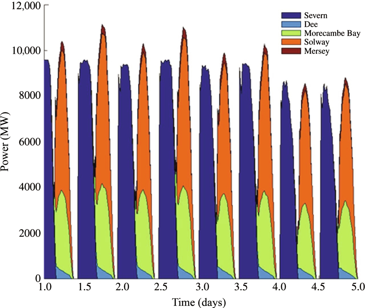
Few studies have considered multiple lagoon operation, never mind multiple lagoon optimization. However, Yates et al. [31] considered (including feedbacks) the operation of five tidal barrages in the Irish Sea, all operating in ebb-only mode. The results show that all of the proposed tidal barrages in the northern part of the Irish Sea (Dee, Morecambe, Solway, Mersey) are in phase with one another, whereas a Severn barrage in the southern Irish Sea is approximately 180 degrees out of phase (Fig. 9.16). This is perhaps not surprising if we examine the M2 cotidal chart of the region (Fig. 9.12). Because the northern part of the Irish Sea is a standing wave system (Section 3.4), there are few cotidal lines in this region (cotidal lines are all 300–360 degrees in Fig. 9.12), indicating that tidal elevations throughout this region are more or less in phase. The cotidal lines in the Severn Estuary have a phase of around 180 degrees in Fig. 9.12, explaining the 180 degrees change in power output between power plants in the southern and northern Irish Sea (Fig. 9.16). However, further optimization (flood-only, ebb-only, and dual model) could be performed on this set of tidal barrages to further smooth power output. Similar optimization could also be performed on multiple tidal lagoon power plants, as considered, in part, by Angeloudis and Falconer [32], who optimized annual electricity production for the Bristol Channel and Severn Estuary. Although they did not optimize to minimize variability of power output, they advise that multiple projects should also consider the environmental consequences of changing the mode of operation; for example, flood-only and ebb-only operation may lead to greater loss of intertidal area and far-field effects, compared with dual-model operation.
9.3.3 Combined Tidal Range and Tidal Stream Phasing
For locations that exhibit an energetic tidal stream and tidal range resource, it is interesting to consider the nature of the tides, as either progressive or standing wave systems. In a progressive wave, tidal elevations and currents are in phase with one another (Fig. 9.17A). High water (HW) is typically a time of standing for a tidal range power plant (Section 3.14), when no electricity would be generated; whereas this is the time associated with peak tidal streams in a progressive wave. Therefore, there is scope for phase diversity between tidal elevations and currents within the same region for a progressive wave system. In a standing wave system (Fig. 9.17B), peak tidal currents occur mid-way between HW and LW, at a stage when a tidal lagoon power plant would be at peak generation (Section 3.14); therefore there is less potential for phase diversity between currents and elevations in a standing wave system. Unfortunately, due to resonance (Section 3.5), most promising tidal range sites will be standing wave systems, hence minimizing the potential for developing combined tidal range and tidal stream power plants at the same location.

9.4 Optimization of Hybrid Marine Renewable Energy Projects
There are many advantages in colocating or combining marine renewable energy power plants at a single location, such as shared grid infrastructure, common substructure/foundation systems, and smoothing the power output when combining multiple renewable resources [33]. Although one colocated combination was briefly discussed in Section 9.3.3 (tidal range power plants and tidal stream arrays), in this section we focus on the colocation of wind and wave arrays.
9.4.1 Combined Wind-Wave Projects
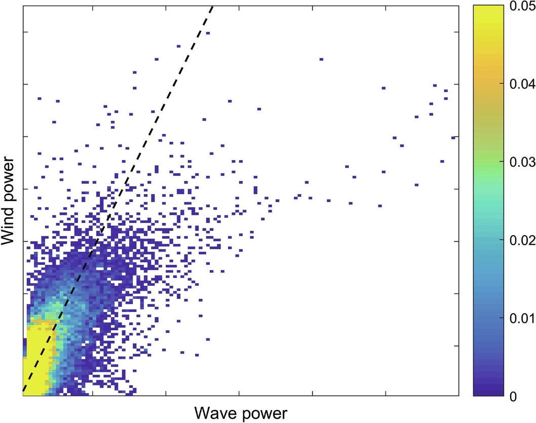
One obvious example where multiple renewable energy resources could be combined at a single location is wave and offshore wind. The offshore wind and wave industries face the same hostile marine environment, and face similar administrative and technological barriers [33]. From a resource perspective, although wind fields lead to the generation of wind waves, often there will be a phase difference or a lag between wind power and wave power, for example, consider the spread of data in Fig. 9.18 calculated for WaveHub, UK. In particular, swell waves are independent of the local wind climate, and so in many ways the wind and wave resource are complementary (although optimization would be required to select the best sites for colocation).
Stoutenburg et al. [35] examined the temporal correlation (Pearson’s) between wind power and wave power at the same and different wave buoys off the coast of California (Fig. 9.19). Lower values (i.e. weakly correlated sites) indicate increased diversity, and so good potential for colocation of wave and wind arrays. Aggregate power from a colocated wind and wave farm achieves reductions in variability equivalent to aggregating power from two offshore wind farms approximately 500 km apart, or two wave farms approximately 800 km apart [35].

In general, a trend of energetic wind and wave activity in winter months coincides with an increased demand for electricity for heating and lighting (e.g. see Fig. 10.1 in the next chapter). However, with significant interannual variability in the wind and wave resources, it is a high-risk strategy to put too much reliance on these stochastic forms of energy conversion. In Fig. 1.12C, we looked at how demand for electricity varied throughout the day, with well-defined peaks at around 08:00 and 18:00. It would therefore be useful if a wind/wave energy mix could be optimized to match these peaks in demand. Cradden et al. [36] considered wind/wave energy mixes in Orkney (at the EMEC wave test site) in the ratios 100% wind:0% wave, 75% wind:25% wave, etc. down to 0% wind:100% wave. Considering only time periods when electricity demand exceeded 90% of peak, the frequency distribution of capacity factor for these different wind/wave energy mixes was calculated (Fig. 9.20). At 100% wind power, there are relatively high frequencies of zero and maximum power, but these two extremes are much less frequent in the 100% wave scenario, indicating that the wave resource is less extreme, but more likely to be present (i.e. more reliable) than the wind resource. A more even distribution across all capacity factors results from all of the combined wind/wave scenarios. However, very specific optimization would be required to determine which of these scenarios is advantageous from both generation and demand perspectives. Further, colocation of wind and wave farms can lead to more complexity in the structural design of the devices due to loading and fluid-structure interactions.

9.5 Optimization Tools
9.5.1 HOMER
Whilst a number of tools are available to optimize distributed and hybrid renewable energy systems, we selected Hybrid Optimization Model for Electric Renewable (HOMER; www.homerenergy.com) as an example to describe some of the capabilities of these tools. HOMER is an example of a computer-based optimization tool developed by National Renewable Energy Laboratory of the US for hybrid renewable energy systems. The main components of this model are simulation, optimization, and sensitivity analysis.
Simulation
Assume that you have designed a configuration for a hybrid renewable energy system. This system has several components such as one or several wind turbines, a storage system (e.g. batteries, hydrogen tank), and diesel generators (for hybrid systems). HOMER simulates the performance of the system every hour for the duration of a year. It calculates the energy produced and compares it with electricity demand. The hourly time series of demand should be provided as an input to the model. HOMER calculates the surplus or deficit at each time step, and tries to address these differences by storing energy during surplus periods, and using stored energy, diesel generators, or grid imports, in times of deficit. Several criteria can be imposed by the user as constraints to determine whether the performance of a system/configuration is acceptable; for example, minimum percent of the time that energy demand should be met, the share of the power supplied by renewable energy (in a hybrid system), and a limit on the emissions can be imposed. In the simulation phase, HOMER also calculates total net present cost of the system (i.e. all future costs are discounted to the present by a discount/interest rate). The costs include initial capital cost, the O&M cost during the lifetime of the project, fuel, and power purchased from the grid. The revenue from selling the power is then subtracted from the total cost to compute the net present cost. LCOE can also be computed given total cost and energy produced during a year.
Optimization
Finding the best configuration of a renewable energy system is the objective of the optimization step. HOMER simulates the performance of several configurations. It selects those that meet the constraints (demand, and minimum percentage of renewable energy contribution in a hybrid system). The best configuration is a solution/configuration that has minimum net present cost. Sample independent (decision) variables that can be changed by HOMER include the number and type/size of wind turbines, the size of the storage system (number of batteries), and the size of diesel generators. A search space that contains all possible scenarios for a component (e.g. various battery sizes) is provided by the user.
Sensitivity Analysis
An optimized system is calculated based on certain assumptions about a number of uncertain parameters; examples are fuel price, grid power price, discount rate, life time of the project, and demand. By performing sensitivity analysis on these variables, a user can deal with uncertainty and understand how/if the optimized system changes with these parameters. For instance, what is the minimum lifetime for a project? What interest rates are feasible for a renewable energy system?
HOMER has been applied in several studies to find the optimum energy system. For instance, in a case study in a remote village in India, four energy sources (hydropower, solar, wind, and bio-diesel generators) were combined [37]. The optimal off-grid system was identified and compared with the alternative of grid extension. This study showed that the hybrid off-grid system is cost-effective, compared with grid extension.
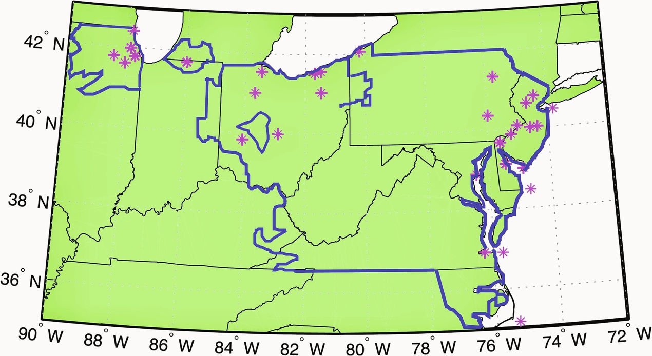
Some studies have optimized energy systems at much larger scales. As an example, Budischak et al. [38] considered a large grid in the eastern United States (Fig. 9.21) with a capacity of 72 GW (PJM Interconnection; www.pjm.com). By combining several renewable energy resources distributed across the region (onshore wind, offshore wind, and solar), and storage systems (batteries and fuel cells), an alternative system based on renewable energy was simulated and optimized. This study proposed an energy system that can meet the electricity demand of this large region based on 90% to 99.99% renewable sources, and with a cost comparable to conventional energy systems by 2030. Notably, Budischak et al. [38] recommended excessive energy production as the least cost option; the renewable system should produce almost three times the electricity demand, on average, to compensate for intermittency, and to avoid high costs associated with energy storage. Offshore wind energy had nearly the same contribution as onshore wind in the energy mix for the 99.99% renewable case in 2030. Both HOMER and another tool RREEOM (Regional Renewable Electricity Economic Optimization Model) were used, whilst PREEOM was recommended for larger grids like PJM.
9.5.2 OpenTidalFarm
OpenTidalFarm is an open source software designed to simulate and optimize arrays of tidal energy converters (TECs; http://opentidalfarm.org). Optimization of TEC arrays generally requires the running of computationally expensive 2D or 3D models, and so only a limited number of options can be explored; for example, Divett et al. [39] explored ‘only’ four TEC array configurations using their 2D shallow water equation model to maximize global array power output. Funke et al. [40] presented an automated procedure for TEC array optimization using the adjoint technique, based on a 2D shallow water equation model. In contrast to less efficient gradient-free optimization algorithms (such as the greedy algorithm presented in Section 9.3.1, which optimizes the objective function, e.g. power output, as a black box), the adjoint method is a gradient-based method. Gradient-based optimization algorithms update the position in parameter space at each iteration using derivatives of the objective function. However, as mentioned before, this involves differentiating through the solution of a partial differential equation, which can be challenging in the case of complex models. In the tidal energy case, we wish to optimize a single variable—power output—with respect to many input parameters, and ‘adjoint linearization’ is a method that can efficiently compute the derivative of a single output with respect to all inputs.
OpenTidalFarm has, amongst other applications, been used to optimize the siting of 256 turbines in the Inner Sound of the Pentland Firth [40], and to minimize the cost of cabling in the same region [12] (Fig. 9.22).
