
This book focuses on using Processing for interactive graphics, because that's the core of what Processing does. However, the software can do much more and is often part of projects that move beyond a single computer screen. For example, Processing has been used to control machines, export images for high-definition films, and export models for 3D printing.
Over the last decade, Processing has been used to make music videos for Radiohead and R.E.M., to make illustrations for publications such as Nature and the New York Times, to output sculptures for gallery exhibitions, to control a 120×12-foot video wall, to knit sweaters, and much more. Processing has this flexibility because of its system of libraries.
A Processing library is a collection of code that extends the software beyond its core functions and classes. Libraries have been important to the growth of the project, because they let developers add new features quickly. As smaller, self-contained projects, libraries are easier to manage than if these features were integrated into the main software.
In addition to the libraries included with Processing (these are called the core libraries), there are over 100 contributed libraries that are linked from the Processing website. All libraries are listed online at http://processing.org/reference/libraries/.
To use a library, select Import Library from the Sketch menu. Choosing a library will add a line of code that indicates that the library will be used with the current sketch. For instance, when the OpenGL Library is added, this line of code is added to the top of the sketch:
importprocessing.opengl.*;
Before a contributed library can be imported through the Sketch menu, it must be downloaded from its website and placed within the libraries folder on your computer. Your libraries folder is located in your sketchbook. You can find the location of your sketchbook by opening the Preferences. Place the downloaded library into a folder within your sketchbook called libraries. If this folder doesn't yet exist, create it.
As mentioned, there are more than 100 Processing libraries, so they clearly can't all be discussed here. We've selected a few that we think are fun and useful to introduce in this chapter.
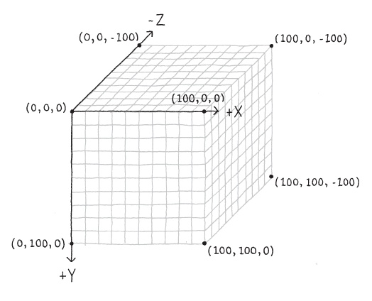
There are two ways to draw in 3D with Processing; both require adding a third parameter to the size() function to change the way graphics are drawn. By default, Processing draws using a 2D renderer that is very precise, but slow. This is the JAVA2D renderer. A sometimes faster but lower-quality version is P2D, the Processing 2D renderer. You can also change the renderer to Processing 3D, called P3D, or OpenGL, to allow your programs to draw in one additional dimension, the z-axis (see Figure 11-1).
Render with Processing 3D like this:
size(800,600,P3D);
And OpenGL like this:
size(800,600,OPENGL);
The P3D renderer is built-in, but the OpenGL renderer is a library and requires the import statement within the code, as shown at the top of Example 11-1: A 3D Demo. The OpenGL renderer makes use of faster graphics hardware that's available on most machines sold nowadays.
Note
The OpenGL renderer is not guaranteed to be faster in all situations; see the size() reference for more details.
Many of the functions introduced in this book have variations for working in 3D. For instance, the basic drawing functions point(), line(), and vertex() simply add z-parameters to the x- and y-parameters that were covered earlier. The transformations translate(), rotate(), and scale() also operate in 3D.
More 3D functions are covered in the Processing Reference, but here's an example to get you started:
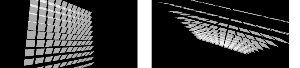
importprocessing.opengl.*;voidsetup(){size(440,220,OPENGL);noStroke();fill(255,190);}voiddraw(){background(0);translate(width/2,height/2,0);rotateX(mouseX/200.0);rotateY(mouseY/100.0);intdim=18;for(inti=-height/2;i<height/2;i+=dim*1.2){for(intj=-height/2;j<height/2;j+=dim*1.2){beginShape();vertex(i,j,0);vertex(i+dim,j,0);vertex(i+dim,j+dim,-dim);vertex(i,j+dim,-dim);endShape();}}}
When you start to work in 3D, new functions are available to explore. It's possible to change the camera, lighting, and material properties, and to draw 3D shapes like spheres and cubes.
This example builds on Example 11-1: A 3D Demo by replacing the rectangles with cubes and adding a few types of lights. Try commenting and uncommenting different lights to see how each works by itself and in combination with others:
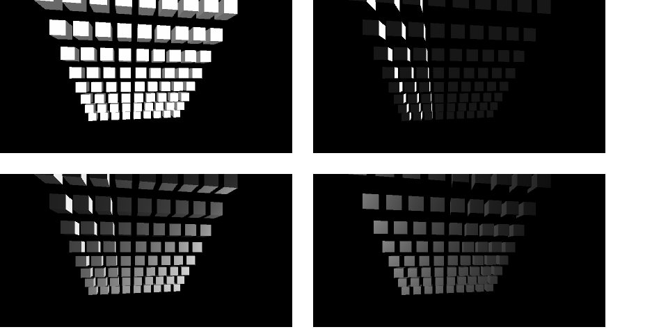
importprocessing.opengl.*;voidsetup(){size(420,220,OPENGL);noStroke();fill(255);}voiddraw(){lights();//ambientLight(102, 102, 102);//directionalLight(255, 255, 255, // Color// −1, 0, 0); // Direction XYZ//pointLight(255, 255, 255, // Color// mouseX, 110, 50); // Position//spotLight(255, 255, 255, // Color// mouseX, 0, 200, // Position// 0, 0, −1, // Direction XYZ// PI, 2); // ConcentrationrotateY(PI/24);background(0);translate(width/2,height/2,−20);intdim=18;for(inti=-height/2;i<height/2;i+=dim*1.4){for(intj=-height/2;j<height/2;j+=dim*1.4){pushMatrix();translate(i,j,-j);box(dim,dim,dim);popMatrix();}}}
There are four types of lights in Processing: spot, point, directional, and ambient. Spot lights radiate in a cone shape; they have a direction, location, and color. Point lights radiate from a single point like a lightbulb of any color. Directional lights project in one direction to create strong lights and darks. Ambient lights create an even light of any color over the entire scene and are almost always used with other lights. The lights() function creates a default lighting setup with an ambient and directional light. Lights need to be reset each time through draw(), so they should appear at the top of draw() to ensure consistent results.
Working in 3D introduces the idea of a "camera" that is pointed at the three-dimensional scene being constructed. Like a real-world camera, it maps the 3D space into the flat 2D plane of the screen. Moving the camera changes the way Processing maps the 3D coordinates of your drawing onto the 2D screen.
By default, Processing creates a camera that points at the center of the screen, therefore shapes away from the center are seen in perspective. The camera() function offers control over the camera location, the location at which it's pointed, and the orientation (up, down, tilted). In the following example, the mouse is used to move the location where the camera is pointing:
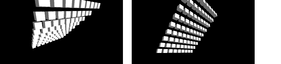
importprocessing.opengl.*;voidsetup(){size(420,220,OPENGL);noStroke();}voiddraw(){lights();background(0);floatcamZ=(height/2.0)/tan(PI*60.0/360.0);camera(mouseX,mouseY,camZ,// Camera locationwidth/2.0,height/2.0,0,// Camera target0,1,0);// Camera orientationtranslate(width/2,height/2,−20);intdim=18;for(inti=-height/2;i<height/2;i+=dim*1.4){for(intj=-height/2;j<height/2;j+=dim*1.4){pushMatrix();translate(i,j,-j);box(dim,dim,dim);popMatrix();}}}
This section has presented the tip of the iceberg of 3D capability. In addition to the core functionality mentioned here, there are many Processing libraries that help with generating 3D forms, loading and exporting 3D shapes, and providing more advanced camera control.
The animated images created by a Processing program can be turned into a file sequence with the saveFrame() function. When saveFrame() appears at the end of draw(), it saves a numbered sequence of TIFF-format images of the program's output named screen-0001.tif, screen-0002.tif, and so on, to the sketch's folder. These files can be imported into a video or animation program and saved as a movie file. You can also specify your own file name and image file format with a line of code like this:
saveFrame("output-####.png");
Note
When using saveFrame() inside draw(), a new file is saved each frame—so watch out, as this can quickly fill your sketch folder with thousands of files.
Use the # (hash mark) symbol to
show where the numbers will appear in the file name. They are replaced
with the actual frame numbers when the files are saved. You can also
specify a subfolder to save the images into, which is helpful when
working with many image frames:
saveFrame("frames/output-####.png");
This example shows how to save images by storing enough frames for a two-second animation. It runs the program at 30 frames per second and then exits after 60 frames:

floatx=0;voidsetup(){size(720,480);smooth();noFill();strokeCap(SQUARE);frameRate(30);}voiddraw(){background(204);translate(x,0);for(inty=40;y<280;y+=20){line(-260,y,0,y+200);line(0,y+200,260,y);}if(frameCount<60){saveFrame("frames/SaveExample-####.tif");}else{exit();}x+=2.5;}
Processing will write an image based on the file extension that you use (.png, .jpg, or .tif are all built in, and some platforms may support others). A .tif image is saved uncompressed, which is fast but takes up a lot of disk space. Both .png and .jpg will create smaller files, but because of the compression, will usually require more time to save, making the sketch run slowly.
If your output is vector graphics, you can write the output to PDF files for higher resolution. The PDF Export library makes it possible to write PDF files directly from a sketch. These vector graphics files can be scaled to any size without losing resolution, which makes them ideal for print output—from posters and banners to entire books.
This example builds on Example 11-4: Saving Images to draw more chevrons of different weights, but it removes the motion. It creates a PDF file called Ex-11-5.pdf because of the third and fourth parameters to size():
importprocessing.pdf.*;voidsetup(){size(600,800,,"Ex-11-5.pdf");noFill();strokeCap(SQUARE);}voiddraw(){background(255);for(inty=100;y<height-300;y+=20){floatr=random(0,102);strokeWeight(r/10);beginShape();vertex(100,y);vertex(width/2,y+200);vertex(width-100,y);endShape();}exit();}
The geometry is not drawn on the screen; it is written directly into the PDF file, which is saved into the sketch's folder. This code in this example runs once and then exits at the end of draw(). The resulting output is shown in Figure 11-2.
There are more PDF Export examples included with the Processing software. Look in the PDF Export section of the Processing examples to see more techniques.

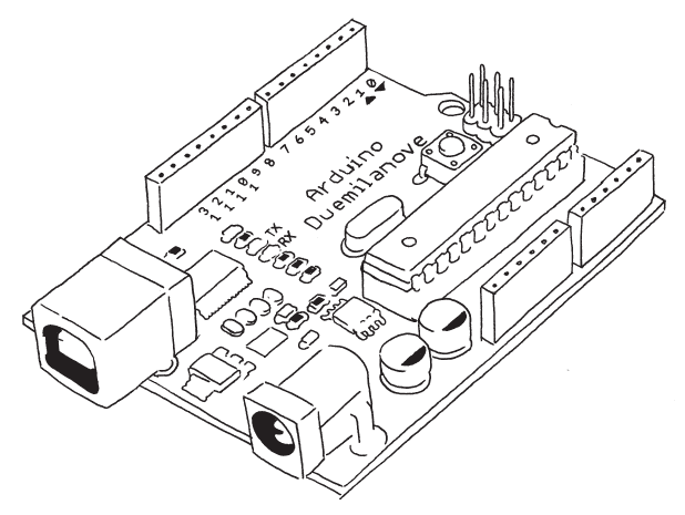
Arduino is an electronics prototyping platform with a series of microcontroller boards and the software to program them. Processing and Arduino share a long history together; they are sister projects with many similar ideas and goals, though they address separate domains. Because they share the same editor and programming environment and a similar syntax, it's easy to move between them and to transfer knowledge about one into the other.
In this section, we focus on reading data into Processing from an Arduino board and then visualize that data on screen. This makes it possible to use new inputs into Processing programs and to allow Arduino programmers to see their sensor input as graphics. These new inputs can be anything that attaches to an Arduino board. These devices range from a distance sensor to a compass or a mesh network of temperature sensors.
This section assumes that you have an Arduino board and that you already have a basic working knowledge of how to use it. If not, you can learn more online at http://www.arduino.cc and in the excellent book Getting Started with Arduino by Massimo Banzi (O'Reilly). Once you've covered the basics, you can learn more about sending data between Processing and Arduino in another outstanding book, Making Things Talk by Tom Igoe (O'Reilly).
Data can be transferred between a Processing sketch and an Arduino board with some help from the Processing Serial Library. Serial is a data format that sends one byte at a time. In the world of Arduino, a byte is a data type that can store values between 0 and 255; it works like an int, but with a much smaller range. Larger numbers are sent by breaking them into a list of bytes and then reassembling them later.
In the following examples, we focus on the Processing side of the relationship and keep the Arduino code simple. We visualize the data coming in from the Arduino board one byte at a time. With the techniques covered in this book and the hundreds of Arduino examples online, we hope this will be enough to get you started.
The following Arduino code is used with the next three Processing examples:
// Note: This is code for an Arduino board, not ProcessingintsensorPin=0;// Select input pinintval=0;voidsetup(){Serial.begin(9600);// Open serial port}voidloop(){val=analogRead(sensorPin)/4;// Read value from sensorSerial.(val,BYTE);// Print variable to serial portdelay(100);// Wait 100 milliseconds}
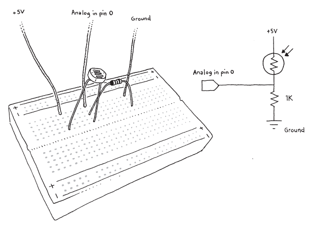
There are two important details to note about this Arduino example. First, it requires attaching a sensor into the analog input on pin 0 on the Arduino board. You might use a light sensor (also called a photo resistor, photocell, or light-dependent resistor) or another analog resistor such as a thermistor (temperature-sensitive resistor), flex sensor, or pressure sensor (force-sensitive resistor). The circuit diagram and drawing of the breadboard with components are shown in Figure 11-4. Next, notice that the value returned by the analogRead() function is divided by 4 before it's assigned to val. The values from analogRead() are between 0 and 1023, so we divide by 4 to convert them to the range of 0 to 255 so that the data can be sent in a single byte.
The first visualization example shows how to read the serial data in from the Arduino board and how to convert that data into the values that fit to the screen dimensions:
importprocessing.serial.*;Serialport;// Create object from Serial classfloatval;// Data received from the serial portvoidsetup(){size(440,220);// IMPORTANT NOTE:// The first serial port retrieved by Serial.list()// should be your Arduino. If not, uncomment the next// line by deleting the // before it. Run the sketch// again to see a list of serial ports. Then, change// the 0 in between [ and ] to the number of the port// that your Arduino is connected to.//println(Serial.list());StringarduinoPort=Serial.list()[0];port=newSerial(this,arduinoPort,9600);}voiddraw(){if(port.available()>0){// If data is available,val=port.read();// read it and store it in valval=map(val,0,255,0,height);// Convert the value}rect(40,val-10,360,20);}
The Serial library is imported on the first line and the serial port is opened in setup(). It may or may not be easy to get your Processing sketch to talk with the Arduino board; it depends on your hardware setup. There is often more than one device that the Processing sketch might try to communicate with. If the code doesn't work the first time, read the comment in setup() carefully and follow the instructions.
Within draw(), the value is brought into the program with the read() method of the Serial object. The program reads the data from the serial port only when a new byte is available. The available() method checks to see if a new byte is ready and returns the number of bytes available. This program is written so that a single new byte will be read each time through draw(). The map() function converts the incoming value from its initial range from 0 to 255 to a range from 0 to the height of the screen; in this program, it's from 0 to 220.
Now that the data is coming through, we'll visualize it in a more interesting format. The values coming in directly from a sensor are often erratic, and it's useful to smooth them out by averaging them. Here, we present the raw signal from the light sensor illustrated in Figure 11-4 in the top half of the example and the smoothed signal in the bottom half:
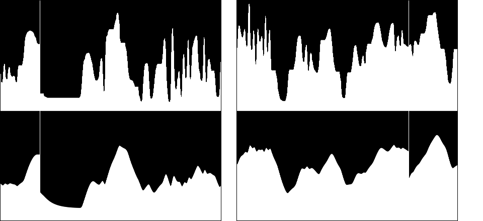
importprocessing.serial.*;Serialport;// Create object from Serial classfloatval;// Data received from the serial portintx;floateasing=0.05;floateasedVal;voidsetup(){size(440,440);frameRate(30);smooth();StringarduinoPort=Serial.list()[0];port=newSerial(this,arduinoPort,9600);background(0);}voiddraw(){if(port.available()>0){// If data is available,val=port.read();// read it and store it in valval=map(val,0,255,0,height);// Convert the values}floattargetVal=val;easedVal+=(targetVal-easedVal)*easing;stroke(0);line(x,0,x,height);// Black linestroke(255);line(x+1,0,x+1,height);// White lineline(x,220,x,val);// Raw valueline(x,440,x,easedVal+220);// Averaged valuex++;if(x>width){x=0;}}
Similar to Example 5-8: Easing Does It and Example 5-9: Smooth Lines with Easing, this sketch uses the easing technique. Each new byte from the Arduino board is set as the target value, the difference between the current value and the target value is calculated, and the current value is moved closer to the target. Adjust the easing variable to affect the amount of smoothing applied to the incoming values.
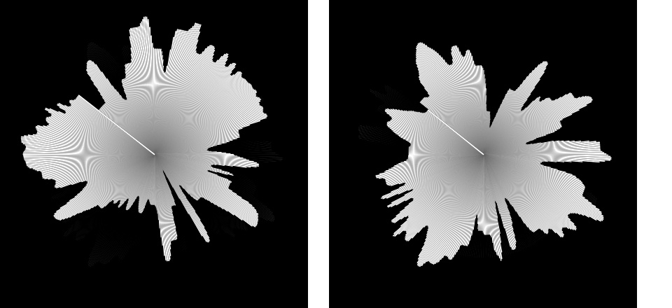
This example is inspired by radar display screens. The values are read in the same way from the Arduino board, but they are visualized in a circular pattern using the sin() and cos() functions introduced earlier in Example 7-12: Sine Wave Values to Example 7-15: Spirals:
importprocessing.serial.*;Serialport;// Create object from Serial classfloatval;// Data received from the serial portfloatangle;floatradius;voidsetup(){size(440,440);frameRate(30);strokeWeight(2);smooth();StringarduinoPort=Serial.list()[0];port=newSerial(this,arduinoPort,9600);background(0);}voiddraw(){if(port.available()>0){// If data is available,val=port.read();// read it and store it in val// Convert the values to set the radiusradius=map(val,0,255,0,height*0.45);}intmiddleX=width/2;intmiddleY=height/2;floatx=middleX+cos(angle)*height/2;floaty=middleY+sin(angle)*height/2;stroke(0);line(middleX,middleY,x,y);x=middleX+cos(angle)*radius;y=middleY+sin(angle)*radius;stroke(255);line(middleX,middleY,x,y);angle+=0.01;}
The angle variable is updated continuously to move the line drawing the current value around the circle, and the val variable scales the length of the moving line to set its distance from the center of the screen. After one time around the circle, the values begin to write on top of the previous data.
We're excited about the potential of using Processing and Arduino together to bridge the world of software and electronics. Unlike the examples printed here, the communication can be bidirectional. Elements on screen can also affect what's happening on the Arduino board. This means you can use a Processing program as an interface between your computer and motors, speakers, lights, cameras, sensors, and almost anything else that can be controlled with an electrical signal. Again, more information about Arduino can be found at http://www.arduino.cc.
We've worked hard to make it easy to export Processing programs so that you can share them with others. In the second chapter, we discussed sharing your programs by exporting them. We believe that sharing fosters learning and community. As you modify the programs from this book and start to write your own programs from scratch, we encourage you to review that section of the book and to share your work with others. At the present, the groups at OpenProcessing, Vimeo, Flickr, and the Processing Wiki are exciting places to visit and contribute to. On Twitter, searches for #Processing and Processing.org yield interesting results. These communities are always moving and flowing. Check the main Processing site (http://www.processing.org) for fresh links as well as these: