
Chapter 13
Testing Data
Summary
This chapter focuses on testing of data. Testing of data involves checking data that the team receives to detect defects. These defects can arise at data extraction, data receipt, and at data load into the team’s Data Manipulation Environment (DME).
You will learn about the five ways in which data can be tested in Guerrilla Analytics. These are (1) completeness, (2) correctness, (3) consistency, (4) coherence, and (5) accountability. This chapter will also describe some tips for successful data testing including scopes of tests, storage of test results, common test routines, and automation of testing.
Keywords
Testing
Coherence
Data
Completeness
Correctness
Accountability
13.1. Guerrilla Analytics workflow
Figure 47 shows the Guerrilla Analytics workflow. Data testing happens at steps 1, 2, and 3 of this workflow. This is because data testing is about increasing confidence in the data received by the analytics team.
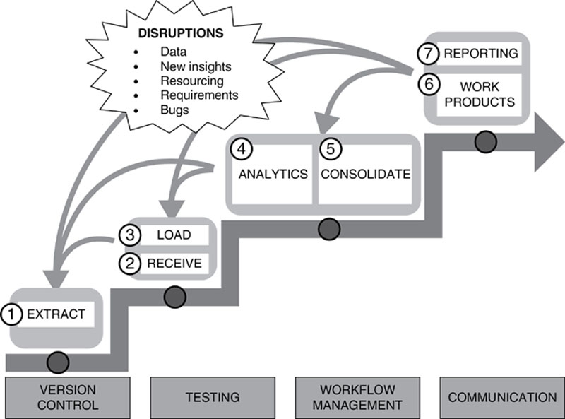
Figure 47 The Guerrilla Analytics workflow
The journey of data as it makes its way to the analytics team follows three key stages.
• Extraction from “source”: Data begins in some “system” which we will refer to as its source. This might be a system in the familiar sense such as a warehouse, a database, a file share, or a content management system. It may also be some type of online web page or application from which data is “scraped.” Even data created by manual data entry is a type of source. Data needs to be taken out of these sources so analytics can be applied to it. It is assumed that there has been a previous exercise with the customer to identify the most appropriate data for the project.
• Transfer to the analytics team: Next, the data needs to be transferred to the analytics team. The complexity of this step varies. If the analytics team is doing web scraping, for example, then the “transfer” is simply the downloading of scraped web pages. However, it is also possible for customers to run their own data extractions from their systems and provide this data to the team. These extracts of data need to be transferred to the analytics team, logged, and stored in a way that data provenance is preserved.
• Loading into the “target” analytics environment: The analytics team then needs to do something with this data. Generally this means loading data into some type of analytics tool where the data can be manipulated and analyzed. The place this data gets loaded into is the “target.”
Data can be corrupted or lost at every stage of the journey from source to target. Even if corruption or loss does not occur, accountability and traceability of the data must be maintained from source to target.
13.2. The five C’s of testing data
The book “Bad Data Handbook” (McCallum, 2012) has a very insightful chapter called “Data Quality Analysis Demystified.” Gleason and McCallum introduce their 4 C framework of data quality analysis. This chapter borrows their four Cs of Completeness, Coherence, Correctness, and aCcountability and adds a fifth C of Consistency. This section will also expand on the five Cs with specific test details and practice tips as appropriate in a Guerrilla Analytics project.
At a high level, the five Cs can be summarized as follows.
• Completeness: Do I actually have all the data I expect to have?
• Correctness: Does the data actually reflect the business rules and domain knowledge we expect it to reflect?
• Consistency: Are refreshes of the data consistent and is the data consistent when it is viewed over some time period?
• Coherence: Does the data “fit together” in terms of its expected relationships?
• ACcountability: Can we trace the data to tell where the data came from, who delivered it, where it is stored in the DME, and other information useful for its traceability?
These are quite straightforward concepts at a high level. You will soon see the variations and subtleties that arise when you try to wrap tests around these concepts and specify expected values for your tests. The subsequent sections now examine the five Cs.
13.3. Testing data completeness
Data Completeness can be thought of as knowing whether you really have all of the data you expect to have. This raises the question of where expectations about the data come from and what they might be. You may be wondering how it could arise that data is not as described. Extracting data from a system is simply a matter of running a query against a database table, right? Actually, loss of data at extraction and at load time can happen for many reasons in real-world scenarios.
The team who extracted the data from the source system may have made a mistake in their extraction code. This has the result that the expected range of data is wrong or particular data fields and tables are missing or corrupted. Database administrators are more used to stuffing data into databases and maintaining database performance. It is rarely their role to pull data out of databases into text files and other file formats.
Even when the correct ranges of data and the correct data fields are present, the fields may not have been populated correctly. Formats of dates and numbers can be corrupted at extraction or inconsistent with expectations. Long text values can end up being cut short. Records can be wrapped and incorrectly delimited. Extraction from other sources such as web pages and file shares is quite ad-hoc as these sources vary so much. How does your team know that all of the source data has been extracted?
The approaches to testing data completeness for structured and unstructured data are slightly different and so we will now deal with them separately.
13.3.1. Approach to Structured Data
The approach to testing completeness of structured data involves two checks.
• Width: Establish and agree the data fields that are to be provided.
• Length: Establish and agree a checksum for each of the data fields of concern.
The first of these tests is straightforward. The data provider communicates the data fields they are going to provide and the data receiver (the analytics team) checks that all those fields are in the delivered data.
The second test is a little more involved. Before discussing the process though, we need to first understand a “checksum.” A checksum is some type of sum or calculation that is performed across every record of a given data field. This effectively summarizes a collection of values from a data field into a single number.
Figure 48 shows a simple checksum for two data fields, a customer name, and a number of visits. The number of visits field, being a number, has simply been summed down the entire data field to give a total of 105. The customer name field, being text, is treated slightly differently. Here the length of each word is summed down the entire data field. Churchill (length 9), Athens (length 6), and so on are summed to give a total of 27.
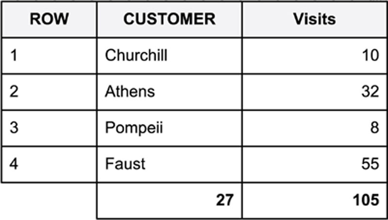
Figure 48 A checksum example
The process for checking data completeness is then the following.
• The data provider calculates checksums as per an agreed definition on their source system.
• The data provider then extracts the data from the source system.
• Data is transferred to the analytics team and loaded onto the target system.
• The analytics team calculates the same checksums as per the agreed definition on their target system.
• The checksums from the source system and the target system are compared to see if there is any difference. A difference in checksums means that the data has changed during its journey from source to target system.
The following sections provide some tips on testing structured data completeness according to this process.
13.3.2. Practice Tip 66: Capture Checksums before Data Extraction
Even when teams do perform checksum calculations, they often slip up on the timing of the calculation. Think about the process that is being followed. Data is being extracted from a source system. The source system is probably live and so new data is being added to it all the time. The checksums calculated on the source system today could be very different to the checksums calculated tomorrow or even an hour later.
It is important that checksums are calculated on the source system at the time of data extraction. This ensures that there is a baseline checksum for comparison against when the data is imported into the target system. Going back to the source system at a later date and trying to retrieve checksums for the data extract is usually difficult. The data will have moved on significantly and there is increased disruption for the customer.
13.3.3. Practice Tip 67: Agree an Approach to Blank Data
Blank data is different from NULL data. While a NULL field will not contribute to a checksum, a blank value might make a contribution depending on how the teams agree to handle blanks.
For example, if a text field contains nothing except 4 blank characters, should its length be reported as 4 or as 0? If a text field has leading or trailing blanks, do they contribute to the field length calculation?
Make sure that the checksum definitions explicitly define how blank and NULL data should be handled.
13.3.4. Practice Tip 68: Allow a Threshold Difference for Some Checksums
Some checksums such as the length of a text field can be calculated precisely. They should not differ between source and target system provided that the checksum is well defined. However, other data types such as floating point numbers can be expected to differ between systems. In practice, you will find that checksums for these data types will differ by a very small amount.
A sensible approach is to agree an allowed threshold for the difference in checksums for data types that vary between source and target systems.
13.3.5. Approach to Unstructured Data
When dealing with unstructured data, the concepts of tables and fields no longer apply. A paragraph of text with embedded tables and perhaps other formatting does not lend itself to a typical checksum. However, it is still important to test that the data has not been modified between extraction and receipt.
Here, the best approach is to create a hash of each dataset. A hash function takes a block of data of arbitrary length and converts it into a number of fixed length. In practice, this means that a file of unstructured data can be summarized by a single number calculated by a hash function. If the contents of the data file change in any way, the number generated by the hash function also changes and you know the data has been modified.
13.3.6. Practice Tip 69: Agree and Test the Hash Function
There are many available hash functions and versions of hash functions. A quick search will yield common functions such as MD5 and SHA as well as their variants such as SHA-1, SHA-2, etc. The implementation of these algorithms should be standardized so that they perform consistently between implementations in various programming languages. If hashes are being calculated by two different teams, it is prudent to agree the specific hash function being used and test that both teams’ implementations are the same.
13.3.7. Why Not Use Hashes in Checksum Calculations?
In the earlier discussion of checksums for structured data, we went to some length to emphasize the importance of defining a checksum for a given data type and how this checksum must then be calculated for all important data fields. You may wonder why we would not recommend using a hash function for a data field or indeed using a hash function for an entire dataset. There are several good reasons for using checksums rather than hashes.
• Hash functions depend on data order: A hash function’s output is dependent on the order of the data that is fed into the function. This means that checksums of data fields using a hash function would have to be careful to order the rows of data consistently in the source and target system. A checksum using a straight forward total does not depend on the order of data rows.
• Hash function implementations may differ between systems: Despite standardizations of hash functions, there is still a good chance that implementations of hash functions may differ between systems or that a particular hash function is not available in one of the source or target systems. Simple sum calculations do not have this limitation.
• Hash functions take longer to compute: A hash function is designed with additional characteristics. Without going into the involved mathematical details, hash functions are designed to produce outputs with a very high probability of uniqueness and certain distribution characteristics. This adds to their computational complexity and execution time. This can be significant when calculating hashes for a large number of data fields in large datasets.
• Hash functions are less informative: A hash function produces a single number as its output. If two data fields differ, two different hash numbers will be produced. However, the difference between these numbers is no indication of how different the data fields are because of how hash functions are designed to work. By contrast, using sums gives a rough measure of how different two compared data fields are.
13.4. Testing data correctness
Data correctness can be thought of as knowing whether the data actually describes the expected business rules. As with completeness, you may wonder how incorrect data could get into a system in the first place. Unfortunately, the all too common reality is that most real-world data contains some amount of incorrectness and so we must test around this to try and detect and quantify it.
Humans enter incorrect data into systems. For example, you may see all sorts of variations for an unknown value such as “N/A,” “UNKNOWN,” “Not Known.” Data fields sometimes get reappropriated for another purpose because of insufficient IT budget or business appetite to reengineer the existing database. Poor application interface design can lead to inappropriate data entry and misuse of data fields. I recently encountered a user “Testy McTestPerson” in some data. Apologies Testy if you are a real person.
Testing data correctness amounts to profiling data fields. That is, you create measures of characteristics about the data field contents. The most relevant types of tests for Guerrilla Analytics come from the field of data quality (Sebastian-Coleman, 2013). These can be categorized as follows.
• Metadata characteristics: These are descriptions of the data itself. There is one piece of metadata that is of most importance in Guerrilla Analytics.
• Data Types: These are the types of data stored in fields such as dates, integers, text, bits, and so on.
• Field Content Characteristics
• Lists of values/labels allowed in a field.
• Formats such as number of decimal places or ordering of day, month, and year in a date.
• Statistics describing the distribution of contents of a data field.
• Dataset Combination Characteristics
• Cross-Column Rules look at combinations of field values in a single record.
The following sections will now discuss these tests in further detail.
13.4.1. Metadata Correctness Tests
Metadata is simply “data about data.” In the case of all DMEs, metadata about a dataset includes the names and types of data fields that are present in a dataset. Most DMEs allow metadata to be queried. It is therefore a simple query to extract the metadata for all datasets and compare it to expectations.
For example, you would expect a date field to have a type of DateTime, Date or some other recognized data type. You would expect a count field to have a type of integer. Occasionally, these expected types are well described in the source system documentation but this should not be assumed to be correct in a Guerrilla Analytics environment.
This type of data correctness information can be compared to documented specifications and validated with business domain experts to test how closely the data matches expectations.
13.4.2. Field Content Correctness Tests
Field content correctness tests, as the name suggests, test the contents of data fields. The scope of testing here is as varied as the data that can be stored in data fields. The following sections describe some of the key types of tests a Guerrilla Analytics team needs to be familiar with.
13.4.2.1. Date Data
Most problems associated with date data can be identified by profiling the distribution of dates in a field.
• Default values: These often show up as the earliest or latest date in the field and stand out because they are significantly different from the rest of the genuine data. For example, 1st January 1900 should be conspicuous if all other data begins in 2013.
• Typos: Confusion about various date formats is common in data entry. For example, a United States user would read 12/10/2014 as December 10th, whereas a British user would read this as 12th of October.
• Sense checks: A dataset of last year’s financial data should not have dates from 10 years ago. A dataset of young adult social media habits should have birth dates from about 15 to 25 years ago.
• Sequences: Working with dates and times suggests the idea of sequences of events. This can be used to assess data correctness. For example, a customer on-boarding date is expected to be earlier than any customer purchase dates.
13.4.2.2. Invalid Values
Some data fields are used to store a particular set of values. A survey question’s answer field may be designed to hold the values “Yes” or “No” but not “Y” or “N.” There is, therefore, an expectation about the contents of these fields that you should test.
• Allowed values: A field to store a RAG value (Red, Amber, Green) should not contain Blue or any other value.
• Invalid values: You will very often find values such as TEST or DO NOT USE, as happened to Maggie in the previous war story 14.
• Invalid ranges: For fields that are a continuous number (as opposed to a list of labels) there may be an allowed range of values that the field can have. For example, a negative payment might not be permitted. A person’s age over 120 would be unusual.
13.4.2.3. Profiling
Even if a field is populated entirely with allowed values, the distribution of those values may not be correct. This is where profiling is important. Calculating distributions of each variable value within a field reveals the frequency of each unique value in the field. Having calculated a distribution, the following analyses can then be applied.
• High-Frequency Values and Low-Frequency Values: The highest and lowest frequency values may be incorrect and should be investigated. After dismissing such outliers, the distribution should be checked to ensure that high and low frequency values are expected from a business perspective. For example, in a distribution of supermarket check-out receipts, you would expect the highest frequency values to be distributed around the average supermarket shop as opposed to small convenience store type purchases.
• Fields with only one value: You will sometimes encounter a field that contains only a single value. This raises the question of what the purpose of the field is. There will be sensible explanations. For example, the field may contain the data processing date or perhaps you are working with a subset of data from a single business region. As with many of these checks, common sense and conversation with the data provider are required.
• Blank fields: A special case of a field with only one value is that where a field is completely NULL or blank. Sometimes fields are deprecated. But sometimes data extraction procedures break and fail to populate a field. When entirely blank fields are detected in testing they should be reported to confirm they are correct.
• Fields with an unexpected number of values: The expectation of high or low numbers of values depends on the purpose of the field. A gender column should only contain male, female, and perhaps unspecified. A column of business products should contain no more values than the total products sold by the business. Variations in the expected number of values can be a sign of incorrect data. For example, three types of values in a field describing activity of an account may lead us to discover correct values of “ACTIVE” and “INACTIVE” as well as an incorrect value such as “NOT ACTIVE.”
13.4.3. Data Combination Correctness Tests
The correctness tests discuss so far have focused on a dataset being set up correctly (metadata correctness) and individual data fields being populated correctly (field content correctness). Within a given dataset, there is another important way in which data may be considered incorrect, even when the metadata and field content tests have passed. You can consider incorrect combinations of values across data fields. Some examples of combinations of exclusive field values follow.
• A medical test particular to male patients should not appear in combination with a patient gender of female.
• A customer purchase order date should not appear in combination with a later customer on-boarding date.
• A customer billing address in the United States should not appear in combination with a customer country identifier of Ireland.
There are also obligatory combinations where the presence of one value necessitates the presence of another value.
• A given postcode/zip code requires a given county in an address.
Needless to say, there are many scenarios here as they depend on the business domain and how it is modeled in the data.
13.4.3.1. Testing Data Combinations
The best way to test for data combination problems is simply to look at all combinations of the data fields in question. The output can then be reviewed to find unexpected and disallowed combinations of data field values.
13.5. Testing consistency
The tests described so far have helped establish confidence in the completeness and correctness of data as a static snapshot. Data consistency can be understood as similarity with characteristics previously observed in the data. Consistency therefore incorporates a time dimension. For example, if the current dataset of website visits has 20,000 hits per day, then an earlier dataset would be expected to a have a similar order of hits per day. The question of data consistency arises in two scenarios encountered in Guerrilla Analytics projects.
• Data refreshes: Data is refreshed during the project because data goes out of date or because additions and changes to the data such as new fields need to be included in an analysis.
• Long time ranges: When a date range for some data stretches over a significant time span, there is a greater chance that business processes might have changed during the course of the data generation. For example, new products were introduced, regional offices were shut down, and significant economic events such as a January sale changed the patterns of data observed.
Consistency testing is about comparing more recent data to that which was seen in the past to detect if patterns in the data have changed over time. The basis of this comparison is similar to many of the tests previously discussed. However, the fact that we are usually comparing data over different time periods forces us to frame these tests slightly differently. Here are the comparisons that can be considered when testing data consistency.
• Consistent field types: If a dataset is refreshed, does it have the same data types as encountered previously? Perhaps text field lengths or numeric types have changed? This issue arises very often in projects where different team members perform the data extraction on separate occasions and do not share the format of the data extracts with one another.
• Consistent rates of activity: Data from an earlier and later time period will obviously have different date values. However, you might expect the rate of activities such as sales or logins to be consistent in both datasets. You could also look for consistency in periodic activities. For example, does account closing always happen within the last 2 days of a month? Is a salary payment always executed on the last Thursday of a month?
• Consistent content: Do fields have the same distribution of values or the same sets of allowed values? For example, a count of the distinct number of staff represented in human resource data should change in line with the business. Unless there has been a dramatic business event, such as an acquisition or rationalization, there should not be significant changes in total staff over time.
• Consistent ratios/proportions: Are the proportions of some combinations of data fields consistent? For example, the number of financial trades per trader or the number of system logins per user per day.
• Consistent summary statistics: Do the sum, range, average, etc. of certain fields remain consistent over particular ranges?
Again, there is potential for much variety in these tests. The intention here is to outline what should be considered. You must then prioritize as appropriate for the given Guerrilla Analytics project.
13.6. Testing data coherence
Data coherence (sometimes called referential integrity) describes the degree to which data relationships are correct and as expected.
In a relational database, each table should have a primary key that uniquely identifies a row of data in that table. The table may also have one or more foreign keys. Foreign keys are a reference to primary keys in other tables. By joining a foreign key to its parent table, a relationship is established between two tables.
Consider the illustrated example in Figure 49. The customer table on the left contains a primary key called CUST_ID that uniquely identifies every customer. It also contains a foreign key called CITY_ID. The CITY_ID is a primary key in its own parent table on the right. These two tables have an expected relationship that every customer lives in only one city.
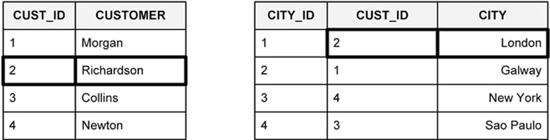
Figure 49 Testing data coherence
Testing data coherence is about establishing (1) whether these table relationships are complete, and (2) whether these relationships are as expected.
13.6.1. Testing Incomplete Relationships
It is expected that any value present in the foreign key column will also be present in the table for which it is the primary key. In the example from Figure 49, every CITY_ID present in the customer table as a foreign key must be present in the city table also. If the value is not present on the parent table then something is wrong with data coherence.
Incomplete relationships can occur for many reasons including problems in data extraction, bugs in the source system, and data purges and archiving processes in the source system. Testing relationships identifies these problems.
13.6.2. Relationships Different from Expectations
There are three basic types of relationships in data that has a relational model.
• One-to-one: An entity in one table is related to only one entity in another table. For example, a given customer can only register one email address with an online shopping site.
• One-to-many: An entity in one table is related to one or more entities in another table. Instances in the other table cannot be related back to other instances in the first table. In effect, the relationship is a hierarchy. A classic example is that of a family tree. A father can have more than one daughter but the daughter cannot have more than one biological father.
• Many-to-many: An entity in one table can be related to many entities in another table and this relationship works in both directions. For example, a supermarket customer can purchase several product types. Each of those product types can also be purchased by many other customers. From a customer perspective, we can say “this customer bought the following products.” Conversely, from the product perspective we can say “this product was bought by all the following customers.”
These types of relationship are sometimes referred to as the “cardinality” of the relationship. Cardinality can easily be tested by joining and counting foreign key to primary key relationships and comparing results to the expected data model.
13.7. Testing accountability
Finally we arrive at data accountability. This is about tracking where data came from. This is more an operational issue in the team’s project management rather than something that is inherent in the data model or data content. To properly track the data you need to be able to say at least the following about it.
• How?
• What queries and process were used to produce the extracted data and are these queries and process repeatable?
• Who produced the data?
• When was the data extract produced?
• What data was produced?
• What source was the data extracted from? This could be a system, file share, email archive, web site, third party, or other data provider.
• What was the scope of the extraction in terms of time, products, customers, regions, or some other business domain boundary?
• What list of datasets was provided in the extract?
• Where are the raw unmodified datasets stored now?
Since accountability is more to do with data management process than data characteristics, it is more difficult to specify automated tests of accountability. You should put in place frequent audits to check completeness of accountability information and consider making a team member responsible for this.
13.7.1. Practice Tip 70: Use a Data Log
Data tracking information for accountability is best stored in a data log which describes the contents of an accompanying data folder. Lightweight methods for tracking data extraction, data receipt, and loading were discussed in an earlier chapter on Data Receipt. At its most basic, a data log can be implemented in a spreadsheet. If available, workflow management tools (Doar, 2011) can also be customized to track data and make individuals accountable for data provenance.
13.7.2. Practice Tip 71: Keep it Simple
Sometimes, the temptation is to try to capture everything you can about the data. Remember the over-arching Guerrilla Analytics principle of simplicity. In a highly dynamic project, there often will not be time or need to capture everything about the data. Focus on the key descriptors that help preserve data provenance.
13.8. Implementing data testing
13.8.1. Overview
So far in this chapter, we have discussed the five Cs of data testing and the various types of tests that can be executed. We have not gone into any details of how these tests would be implemented.
You may have noticed that data testing at a high level amounts to checksums and data profiling. These activities are applied to entire datasets and also fields within datasets and are generally sums, counts, ranges, and other aggregates of datasets and fields.
This section now summarizes some tips for implementing these data tests in a Guerrilla Analytics environment.
13.8.2. Practice Tip 72: Limit Data Test Scope and Prioritize Sensibly
There is a huge scope of tests that can be performed when testing completeness, correctness, coherence, consistency and accountability. You could profile every data field, enumerate the contents of every field and test every dataset join. Bear in mind that tests are like all code and so have a maintenance cost. Tests have to be maintained and then rerun and reviewed as frequently as the data changes. There is a judgment call to make on the balance between testing every aspect of your data and exhausting project resources versus doing enough testing to cover critical defects. The Guerrilla Analytics environment often limits the sophistication of data profiling tools available, if any, and the time you can use in data testing. To help prioritize data testing, ask questions such as the following.
• Which data joins are critical in rebuilding any relational data?
• Which fields are used in business rules and so influence calculations and filtering?
• Which fields appear in customer outputs and so must be correct?
• Which datasets are being refreshed and are expected to remain consistent across refreshes?
Keeping agility in mind, the critical tests can be built first and additional tests added as resourcing and project requirements dictate. This leads to the next testing tip.
13.8.3. Practice Tip 73: Design Tests with Automation in Mind
Data refreshes of even moderate size and complexity can contain hundreds of datasets. Manually running tests for each of these datasets is not practical. The latest results have to be inspected in addition to a comparison with the results of the previous test run. The best approach is to automate test execution, as is done with test harnesses in traditional software engineering (Tahchiev et al., 2010).
A strategy for test automation requires the following automation features.
• Test scripts can be easily identified and executed: Test scripts can then be automatically picked up and executed with a command line script or scripting language.
• Test results are written to a consistent location with a consistent format: Test results can then be inspected and reported on automatically.
Setting aside project time to program this automation greatly diminishes the testing burden and thereby encourages the team to run critical tests frequently rather than postpone them. The team need only inspect test outputs when tests fail. This frees them up to either refine tests, increase test coverage, or do other analytics work.
13.8.4. Practice Tip 74: Store Test Results Near the Data
Data testing is a critical activity. If errors are discovered in test results, and mistakes in business rules are ruled out as a cause of error then the data itself will come under scrutiny. Even though the analytics team does not generate the raw data, there is a responsibility on them as domain experts to test the data they receive and avoid wasting time on analyses that cannot be used. Despite this responsibility, teams very often run data tests in an ad-hoc fashion, manually inspecting results, and then discarding results.
Test results should be stored in a way that the tests done on a particular dataset can easily be located without the overhead of unnecessary documentation. One method is to place test results in a dataset with a similar name to the dataset being tested. For example, checksums on a dataset called FX_TRADES could be stored in a dataset called FX_TRADES_TEST. You may wish to locate these test result datasets in the same namespace as their target datasets or you may want to file test results in another location. The key here is to have a team convention that makes test results for a given dataset or field easy to locate, ideally with minimal documentation overhead.
The main advantage of storing test results in the DME is that the team can quickly inspect, query, and report on test results without having to leave the DME. This is useful for quickly preparing data quality reports and for reporting on any differences between data refreshes.
13.8.5. Practice Tip 75: Structure Data Test Results in a Consistent Format
If the team is following the good practice of keeping all test results in test datasets, it would also be beneficial to structure these tests results in a similar format.
Establish a dataset of test metric definitions. This should contain at least a metric ID, metric name, and metric description. Each test result dataset should then contain some of the following fields.
• Metric ID: This is a reference to the metric definition table.
• Dataset name: This is the dataset being tested.
• Dataset source: This is a reference to the dataset source. This may be needed if the source cannot be identified from the dataset name.
• Expected value: For the given test metric, this lists the expected value of the test.
• Actual value: For the given test execution, this records the actual value that was calculated by the test.
• Timestamp: This records when the particular test was run and the result was recorded.
• Pass/fail: This records whether a particular test run passed or failed.
• Reason: This is a short business description of why a test failed.
The exact format may differ between types of tests. For example, a coherence test would need to list both the dataset on the left of the join and the dataset on the right of the join.
If test datasets have a common format then automated reporting across test datasets is far easier. This saves precious time in a Guerrilla Analytics project.
13.8.6. Practice Tip 76: Develop a Suite of Test Routines
Data testing does not need to occur at a daily or even weekly frequency. Since data testing is about finding defects in data that comes to the team, these tests need only be run once when new data is delivered to the team. Furthermore, there is a lot of repetition within tests. You always look at aspects of the data such as:
• Comparisons of primary and foreign keys.
• Distribution of values.
• Lists of allowed data values.
• Grouping of combinations of multiple fields.
These common patterns cry out for some common team code for running these types of tests. Such code could have the following types of functionality.
• Given a dataset and foreign key field and another dataset in which that foreign key is the primary key, do a comparison of the values in the foreign key and primary key field.
• Given a field of data, list all unique values and compare to a list of expected values.
• Given a date, numeric, or text field, calculate an appropriate checksum.
There are sophisticated data profiling tools that will do all of this and more. Again, in a Guerrilla Analytics project you should expect that available tool sets will be limited and so you need to think about the priority test functionality that can be automated by your team with minimal overhead.
13.9. Wrap up
This chapter has described testing of data. In this chapter you have learned the following.
• The five Cs of data testing which are Completeness, Correctness, Consistency, Coherence, and aCcountability.
• Completeness testing checks whether the team has received the expected data fields and that the data as it left the source system is unchanged from the data that was loaded into the team’s target DME.
• Correctness testing covers the following.
• Metadata testing checks whether data fields are of the expected data types such as date, numeric, and text.
• Field content testing asks whether data fields have expected content.
• Combination tests check whether expected combinations of values in multiple fields occur together.
• Consistency tests check whether the characteristics of the data have changed significantly over some period of time and one or more data refreshes.
• Coherence or Referential Integrity tests check that table relationships are correct. Foreign keys must exist as primary keys in some table and the expected cardinality of data relationships must be respected.
• Accountability tests check that all the relevant detail is present to track where data came from.
• Recommended data structures and locations for storing test results were discussed. In particular, it was emphasized that test results should be stored near the datasets they test and should be structured in a consistent format.
• Automating test execution means that tests can easily be repeated with data refreshes. Removing the manual process of running tests reduces the temptation to postpone testing and reduces the risk of omitting tests when running a large number of test scripts.
..................Content has been hidden....................
You can't read the all page of ebook, please click here login for view all page.