
Appendix
Data Gymnastics
Data gymnastics patterns
It is of not much help to say “be good at hacking” or “learn {insert data language of your preference/bias}.” I know that whenever I begin to learn a new language, I find it frustrating. I know what I want to do with the data but I lack the vocabulary and the expressiveness in my new language to actually execute what I want to do. The peculiarities of Guerrilla Analytics make it difficult to find advice on what to learn in traditional books on data manipulation.
What follows are the most common patterns your team will encounter time and again in Guerrilla Analytics work. A top performing team will have one or more people who can quickly recognize and execute these patterns in the team’s Data Manipulation Environment (DME) of choice.
Pattern 1: Dataset Collections
Data often needs to be sifted through and broken out into different buckets. You may need to track versions of data and versions of analyses. You may need to identify subsets of data.
This pattern means having a method to place certain datasets matching a pattern into a collection so they can be considered together. Some examples include the following.
• Creating views over a subset of relational tables and schemas that match a pattern.
• Moving tables and views between database schemas.
• In a document database (Sadalage and Fowler, 2012), this could mean creating collections and placing documents into these collections depending on certain document properties.
• In a graph database (Sadalage and Fowler, 2012), this may mean labeling nodes and edges so they can be grouped together.
Whatever the DME, the analyst must have a method to form data collections.
Pattern 2: Append Data Using Common Fields
Data is often broken up into many datasets. For example, log data is often written into daily files. To analyze a year of logs you would have to put all these files together end to end. Occasionally, data needs to be broken into chunks to help it load successfully into the DME and then appended together once safely in the DME.
You need to be able to stick datasets together end to end. What makes this a little more challenging is that the various dataset you are appending may not all have the same fields. Lining up these fields manually in code quickly becomes very cumbersome and error prone. Figure 63 shows a simplified relational database example. On the left are two datasets from two different financial trade systems. You need to append these together so that all common fields line up and the remaining fields are kept in the final appended dataset. One of the datasets has a field called TRADE_DT while in the other it is called DATE. The other fields are common to both datasets although the STATUS field seems to have a different range of values. On the right is the desired result. This result dataset has all the fields of both datasets. Where fields are common (ID, STATUS, and VALUE), they have been lined up. Where fields are different, they have been blanked out in the dataset they do not exist in. There is more work to do of course. TRADE_DT and DATE should now be combined and the coding of STATUS should be unified, for example. However, having the ability to quickly append datasets and not lose information has removed what is normally a cumbersome and error-prone process.
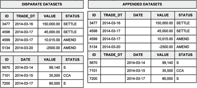
Figure 63 Appending data with common fields
Pattern 3: Map Fields to New Field Names
As discussed already, data can arrive chunked into a number of separate datasets that must be appended together. In addition, these individual datasets may have different names for common fields. For example, a customer identifier field in one dataset may be called “ID” but may be called “CUST_ID” in another dataset. This quickly becomes difficult when you are faced with a large number of datasets and a large number of differing field names.
Figure 64 illustrates what this looks like. The mapping dataset defines a list of original field names and their target new names in the “FROM” and “TO” fields, respectively. The original dataset is passed through this mapping dataset to give the output at the bottom of the figure. Any fields mentioned in the mapping dataset have now been renamed. Other fields such as “CUSTOMER” have been ignored. The mapping dataset is a convenient reference dataset that can be version controlled and signed off by the customer.
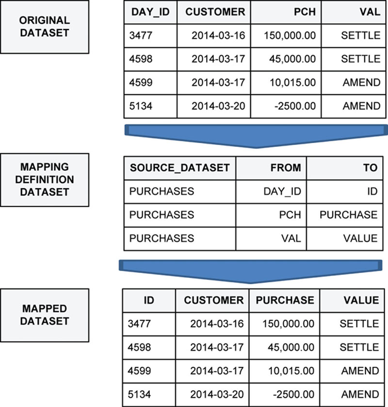
Figure 64 Map fields to new field names
Pattern 4: Identify Duplicates Without Removing Data
Time and again you will encounter duplicates in data. You know from earlier chapters that it is preferable to flag duplicates rather than delete them outright as this preserves data provenance.
This pattern involves being able to identify and flag all duplicates in a dataset using some or all data fields. Figure 65 shows an illustration of what this looks like. The dataset on the left contains five records. Two of these are duplicates. A common approach is to compare records across columns and removed any duplicates detected. The Guerrilla Analytics approach instead flags duplicate groups as shown in the dataset on the right. The “GROUP” field is an identifier for duplicate groups found in the data. Records that are deemed to be duplicates of one another are given the same group identifier. Records within a group are numbered. With this approach,
• Duplicates are visible in the data and can be inspected.
• Deduplicating the dataset is a simple matter of selecting the first member from each duplicate group.
• Duplicate group sizes can be calculated to prioritize the areas of the data that have the largest duplicate issues.
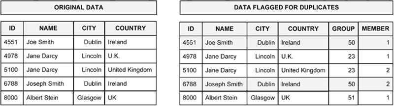
Figure 65 Identify duplicates without removing data
Pattern 5: Uniquely Identify a Row of Data With a Hash
Because you are often extracting data from a multitude of disparate sources, these sources will either have completely incompatible ID fields or will have no ID at all such as in the case of web pages and spreadsheets.
A key skill is the ability to deterministically ID a row of data. The best way to do this is with a hash code. However, it is not simply a matter of applying a hash function (if one is available in the DME). How are blanks and NULLs handled? How should the data be parsed so that every row’s calculated hash code is unique? Team members need to have access to and understand how to consistently use a hash function for row identification.
Pattern 6: Summarize Data
It is critical for reporting, data exploration, and data testing that an analyst can summarize data quickly. Some useful summaries that an analyst should be able to produce are:
• Date and value ranges.
• Counts of labels, both overall and unique.
• Sum, average, median, and other descriptive statistics.
• Placing data records into quartiles, deciles, etc.
• Ordering data by time or some other ordering field and then selecting the Nth item from that ordered list.
• Listing the field types and field names in all datasets.
Pattern 7: Pivot and Unpivot Data
A natural relational structure or document structure is very often not how data gets reported. People prefer data organized in pivoted tables. Conversely, data often arrives with a team in this presentation format and needs to be unpivoted before it can be used. This is typical with survey data, for example. Analysts need to be able to move data back and forth between these two formats quickly in program code.
Pattern 8: Roll Up Data
Data can be provided such that a key field has values split across many rows.
Figure 66 shows a typical dataset representing a simplified transaction log. The transaction log has been sorted by user and by event so that all events for a given user appear in event order beside that user. The user “Andrea Lazar” has three events and Albert Stein has two. Now, in many applications and for some presentation purposes you should like to produce the dataset shown in the right of the figure. All events associated with each user have been “rolled up” onto a single row separated by a “/”delimiter. It is now a simple step to produce one row of data per unique user.
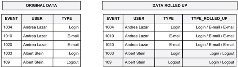
Figure 66 Roll up data
Pattern 9: Unroll Data
Unrolling data is the exact opposite of “rolling up data.” In this case, data is provided rolled up in some type of delimited format such as the “/”delimiter of the previous example (see Figure 66). The objective is to break this out into a new row for every item in the delimited list.
Pattern 10: Fuzzy Matched Data
When bringing together disparate data sources, it can happen that they will not have a common join key that can be used. In these cases you must resort to fuzzy matching the datasets against one another. Fuzzy matching is simply a way of comparing two pieces of text and measuring how similar they are. For example, “bread”and “breed” are very similar because they differ only by one letter in the same location. “Bread” and “butter” however are less similar.
Figure 67 illustrates two datasets that are fuzzy matched into a new result. At the top of the figure are two source datasets that must be joined together. They have come from different systems and so do not share any common key that would permit the usual joining together of datasets. On the left is a list of actor names and their country of residence. On the right is a list of typed actor names (with typos) and the year of the actor’s last film. After fuzzy matching the two datasets on actor name, you see the result at the bottom of the figure. Schwartzeneggar has not been matched to anything. Gleeson and Downey have been matched to two candidates in decreasing order of similarity.
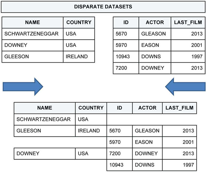
Figure 67 Fuzzy-matched datasets
The technical and mathematical details of fuzzy matching are beyond the scope of this book. However, the analyst needs to be familiar with the use of fuzzy matching algorithms, how they can be tuned, and how to interpret their outputs.
Pattern 11: Fuzzy Group Data
Fuzzy grouping is closely related to fuzzy matching. Fuzzy grouping occurs when you want to find similar groups of data records or documents within the same dataset. This may be because you are looking for duplicates or because you are interested in similar groups. Fuzzy grouping is effectively a fuzzy match where the dataset is fuzzy joined on itself to determine how similar a dataset’s records are to one another.
Pattern 12: Pattern Match With Regular Expressions
When searching data, parsing it and doing certain types of matching, it is useful to be able to identify patterns. This is where regular expressions come into play. Regular expressions (Goyvaerts and Levithan, 2009; Friedl, 1997) are like a language that allows you to succinctly express text-matching conditions. For example, imagine trying to match all email addresses in some data. If you attempted a procedural approach to this problem it would require a significant amount of program code. You would have to iterate through each piece of text looking for a single “@” symbol followed by several letters, a “.” symbol and then some more letters. Having found that, you would then need to go back and capture the entire string of text containing this pattern.
Regular expressions instead allow you to succinctly express a pattern matching string that can catch all variants of email addresses using a rule such as “must contain the @ character followed by some amount of characters including at least one “.” after the “@” symbol.” Other examples of where regular expressions are very useful are:
• Find valid postcode and zip code patterns.
• Determine if a transaction code matches an expected pattern.
• Parse a web log into each of its fields such as timestamp and return code.
• Parse a name field into first name, optional middle name, and last name separated by a comma or one or more spaces.
• Join together two data records where they both contain the string “Name:”
Pattern 13: Select the Previous or Subsequent N records
Time series data is everywhere. Financial transactions, machine logs, website navigation and click through, and shopping checkouts are all time series data. Over time, some set of activities occurs and you would like to better understand patterns and trends in those activities. In these problems, it is necessary to “look back” into the data or “look ahead” into the data. That is, you would like to ask questions such as “show me five records previous” for this user or “show me the next record after the current one” or indeed “show me everything that happens between the current record and the next 10 records.”
Pattern 14: Compare Data
Data arrives with the team in many versions and work product iterations. Analysts often struggle to determine if there are differences between datasets and where exactly those differences are located.
An analyst should know how to quickly “diff” two datasets by certain fields and by an entire row.
Pattern 15: Convert All Blanks to Null and Nulls to Blanks
If there is one area that causes more data analytics bugs than any other, it is probably the presence of NULLs and blanks in data. Whether you use one or the other depends very much on circumstances. Regardless, you will need a way to go through data fields and switch all NULLs to blanks and vice versa.
Pattern 16: Checksum Data
The chapter on data testing emphasized the importance of checksums. An analyst needs to understand and be able to quickly calculate checksums on both text files and DME datasets for a variety of data types.
Wrap up
This appendix has described some of the most common data manipulation patterns encountered in Guerrilla Analytics projects. A high-performing team will be able to recognize these patterns and implement them in program code.
..................Content has been hidden....................
You can't read the all page of ebook, please click here login for view all page.