
Multivariable Calculus
Most physical systems are characterized by more than two quantitative variables. Experience has shown that it is not always possible to change such quantities at will, but that specification of some of them will determine definite values for others. Functional relations involving three or more variables lead us to branches of calculus which make use of partial derivatives and multiple integrals.
11.1 Partial Derivatives
We have already snuck in the concept of partial differentiation in several instances by evaluating the derivative with respect to x of a function of the form ![]() , while treating
, while treating ![]() as if they were constant quantities. The correct notation for such operations makes use of the “curly dee” symbol
as if they were constant quantities. The correct notation for such operations makes use of the “curly dee” symbol ![]() , for example
, for example
![]() (11.1)
(11.1)
To begin with, we will consider functions of just two independent variables, such as ![]() . Generalization to more than two variables is usually straightforward. The definitions of partial derivatives are closely analogous to that of the ordinary derivative:
. Generalization to more than two variables is usually straightforward. The definitions of partial derivatives are closely analogous to that of the ordinary derivative:
![]() (11.2)
(11.2)
and
![]() (11.3)
(11.3)
The subscript y or x denotes the variable which is held constant. If if there is no ambiguity, the subscript can be omitted, as in (11.1). Some alternative notations for ![]() are
are ![]() , and
, and ![]() . As shown in Figure 11.1, a partial derivative such as
. As shown in Figure 11.1, a partial derivative such as ![]() can be interpreted geometrically as the instantaneous slope at the point (x, y) of the curve formed by the intersection of the surface
can be interpreted geometrically as the instantaneous slope at the point (x, y) of the curve formed by the intersection of the surface ![]() and the plane y = constant, and analogously for
and the plane y = constant, and analogously for ![]() . Partial derivatives can be evaluated by the same rules as for ordinary differentiation, treating all but one variable as constants.
. Partial derivatives can be evaluated by the same rules as for ordinary differentiation, treating all but one variable as constants.
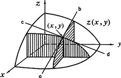
Figure 11.1 Graphical representation of partial derivatives. The curved surface represents ![]() in the first quadrant. Vertically and horizontally cross-hatched planes are x = constant and y = constant, respectively. Lines ab and cd are drawn tangent to the surface at point
in the first quadrant. Vertically and horizontally cross-hatched planes are x = constant and y = constant, respectively. Lines ab and cd are drawn tangent to the surface at point ![]() . The slopes of ab and cd equal
. The slopes of ab and cd equal ![]() and
and ![]() , respectively.
, respectively.
Products of partial derivatives can be manipulated in the same way as products of ordinary derivatives provided that the same variables are held constant. For example,
![]() (11.4)
(11.4)
and
![]() (11.5)
(11.5)
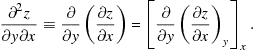
Since partial derivatives are also functions of the independent variables, they can themselves be differentiated to give second and higher derivatives. These are written, for example, as
 (11.6)
or, in more compact notation, ![]() . Also possible are mixed second derivatives such as
. Also possible are mixed second derivatives such as
 (11.7)
When a function and its first derivatives are single valued and continuous, the order of differentiation can be reversed, so that
![]() (11.8)
(11.8)
or, more compactly, ![]() . Higher-order derivatives such as
. Higher-order derivatives such as ![]() and
and ![]() can also be constructed.
can also be constructed.
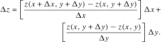
Thus far we have considered changes in ![]() brought about by changing one variable at a time. The more general case involves simultaneous variation of x and y. This could be represented in Figure 11.1 by a slope of the surface
brought about by changing one variable at a time. The more general case involves simultaneous variation of x and y. This could be represented in Figure 11.1 by a slope of the surface ![]() cut in a direction not parallel to either the x- or y-axis. Consider the more general increment
cut in a direction not parallel to either the x- or y-axis. Consider the more general increment
![]() (11.9)
(11.9)
Adding and subtracting the quantity ![]() and inserting the factors
and inserting the factors ![]() and
and ![]() , we find
, we find
 (11.10)
Passing to the limit ![]() , the two bracketed quantities approach the partial derivatives (11.2) and (11.3). The remaining increments
, the two bracketed quantities approach the partial derivatives (11.2) and (11.3). The remaining increments ![]() approach the differential quantities
approach the differential quantities ![]() . The result is the total differential:
. The result is the total differential:
![]() (11.11)
(11.11)
Extension of the total differential to functions of more than two variables is straightforward. For a function of n variables, ![]() , the total differential is given by
, the total differential is given by
![]() (11.12)
(11.12)
A neat relation among the three partial derivatives involving x, y, and z can be derived from Eq. (11.11). Consider the case when z = constant, so that ![]() . We have then that
. We have then that
![]() (11.13)
(11.13)
But the ratio of dy to dx means, in this instance, ![]() , since z was constrained to a constant value. Thus we obtain the important identity
, since z was constrained to a constant value. Thus we obtain the important identity
![]() (11.14)
(11.14)
or in a cyclic symmetrical form
![]() (11.15)
(11.15)
As an illustration, suppose we need to evaluate ![]() for one mole of a gas obeying Dieterici’s equation of state
for one mole of a gas obeying Dieterici’s equation of state
![]() (11.16)
(11.16)
The equation cannot be solved in closed form for either V or T. However, using (11.14), we obtain, after some algebraic simplification:
![]() (11.17)
(11.17)
Problem 11.1.1
For the function ![]() , evaluate
, evaluate
![]()
Problem 11.1.3
For the van der Waals equation of state
![]()
evaluate ![]() .
.
11.2 Multiple Integration
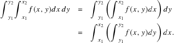
A trivial case of a double integral can be obtained from the product of two ordinary integrals, say
![]() (11.18)
(11.18)
Since the variable in a definite integral is just a dummy variable, its name can be freely changed, say from x to y, in the first equality above. It is clearly necessary that the dummy variables have different names when they occur in a multiple integral. A double integral can also involve a nonseparable function ![]() . For well-behaved functions the integrations can be performed in either order. Thus
. For well-behaved functions the integrations can be performed in either order. Thus
 (11.19)
For well-behaved functions the integrations above can be performed in either order.
More challenging are cases in which the limits of integration are themselves functions of x and y, for example
![]() (11.20)
(11.20)
If the function ![]() is continuous, either of the integrals above can be transformed into the other by inverting the functional relations for the limits from
is continuous, either of the integrals above can be transformed into the other by inverting the functional relations for the limits from ![]() to
to ![]() . This is known as Fubini’s theorem. The alternative evaluations of the integral are represented in Figure 11.2.
. This is known as Fubini’s theorem. The alternative evaluations of the integral are represented in Figure 11.2.

Figure 11.2 Evaluation of double integral ![]() . On left, horizontal strips are integrated over x between
. On left, horizontal strips are integrated over x between ![]() and
and ![]() and then summed over y. On right, vertical strips are integrated over y first. By Fubini’s theorem, the alternative methods give the same result.
and then summed over y. On right, vertical strips are integrated over y first. By Fubini’s theorem, the alternative methods give the same result.
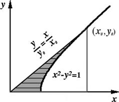
As an illustration, let us do the double integration over area involved in the geometric representation of hyperbolic functions (see Figure 4.17). Referring to Figure 11.3, it is clearly easier to first do the x-integration over horizontal strips between the straight line and the rectangular hyperbola. The area is then given by
![]() (11.21)
(11.21)
where
![]() (11.22)
(11.22)
This reduces to an integration over y:
![]() (11.23)
(11.23)
Since ![]() , we obtain
, we obtain ![]() . Thus we can express the hyperbolic functions in terms of the shaded area A:
. Thus we can express the hyperbolic functions in terms of the shaded area A:
![]() (11.24)
(11.24)
11.3 Polar Coordinates
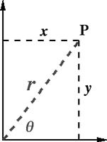
Cartesian coordinates locate a point ![]() in a plane by specifying how far east (x-coordinate) and how far north (y-coordinate) it lies from the origin (0, 0). A second popular way to locate a point in two dimensions makes use of plane polar coordinates,
in a plane by specifying how far east (x-coordinate) and how far north (y-coordinate) it lies from the origin (0, 0). A second popular way to locate a point in two dimensions makes use of plane polar coordinates, ![]() , which specifies distance and direction from the origin. As shown in Figure 11.4, the direction is defined by an angle
, which specifies distance and direction from the origin. As shown in Figure 11.4, the direction is defined by an angle ![]() , obtained by counterclockwise rotation from an eastward heading. Expressed in terms of Cartesian variables x and y, the polar coordinates are given by
, obtained by counterclockwise rotation from an eastward heading. Expressed in terms of Cartesian variables x and y, the polar coordinates are given by
![]() (11.25)
(11.25)
and conversely,
![]() (11.26)
(11.26)
Integration of a function over two-dimensional space is expressed by
![]() (11.27)
(11.27)
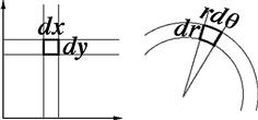
In Cartesian coordinates, the plane can be “tiled” by infinitesimal rectangles of width dx and height dy. Both x and y range over ![]() . In polar coordinates, tiling of the plane can be accomplished by fan-shaped differential elements of area with sides dr and
. In polar coordinates, tiling of the plane can be accomplished by fan-shaped differential elements of area with sides dr and ![]() , as shown in Figure 11.5. Since r and
, as shown in Figure 11.5. Since r and ![]() have ranges
have ranges ![]() and
and ![]() , respectively, an integral over two-dimensional space in polar coordinates is given by
, respectively, an integral over two-dimensional space in polar coordinates is given by
![]() (11.28)
(11.28)
It is understood that, expressed in terms of their alternative variables, ![]() .
.
A systematic transformation of differential elements of area between two coordinate systems can be carried out using
![]() (11.29)
(11.29)
In terms of the Jacobian determinant
![]() (11.30)
(11.30)
In this particular case, we find using (11.26)
![]() (11.31)
(11.31)
in agreement with the tiling construction.
A transformation from Cartesian to polar coordinates is applied to evaluation of the famous definite integral
![]()
Taking the square and introducing a new dummy variable, we obtain
![]() (11.32)
(11.32)
The double integral can then be transformed to polar coordinates to give
![]() (11.33)
(11.33)
Therefore ![]() .
.
Problem 11.3.1
Transform the Cartesian equation for a circle, ![]() , into polar coordinates.
, into polar coordinates.
11.4 Cylindrical Coordinates
Cylindrical coordinates are a generalization of polar coordinates to three dimensions, obtained by augmenting r and ![]() with the Cartesian z coordinate. (Alternative notations you might encounter are r or
with the Cartesian z coordinate. (Alternative notations you might encounter are r or ![]() for the radial coordinate and
for the radial coordinate and ![]() or
or ![]() for the azimuthal coordinate.) The
for the azimuthal coordinate.) The ![]() Jacobian determinant is given by
Jacobian determinant is given by
 (11.34)
the same value as for plane polar coordinates. An integral over three-dimensional space has the form
![]() (11.35)
(11.35)
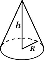
As an application of cylindrical coordinates, let us derive the volume of a right circular cone of base radius R and altitude h, shown in Figure 11.6. This is obtained, in principle, by setting the function ![]() inside the desired volume and equal to zero everywhere else. The limits of r-integration are functions of z, such that
inside the desired volume and equal to zero everywhere else. The limits of r-integration are functions of z, such that ![]() between
between ![]() and
and ![]() . (It is most convenient here to define the z-axis as pointing downward from the apex of the cone.) Thus,
. (It is most convenient here to define the z-axis as pointing downward from the apex of the cone.) Thus,
![]() (11.36)
(11.36)
which is ![]() the volume of a cylinder with the same base and altitude.
the volume of a cylinder with the same base and altitude.
11.5 Spherical Polar Coordinates
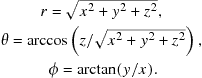
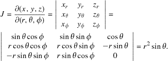
Spherical polar coordinates provide the most convenient description for problems involving exact or approximate spherical symmetry. The position of an arbitrary point P is described by three coordinates ![]() , as shown in Figure 11.7. The radial variable r gives the distance OP from the origin to the point P. The azimuthal angle, now designated as
, as shown in Figure 11.7. The radial variable r gives the distance OP from the origin to the point P. The azimuthal angle, now designated as ![]() , specifies the rotational orientation of OP about the z-axis. The third coordinate, now called
, specifies the rotational orientation of OP about the z-axis. The third coordinate, now called ![]() , is the polar angle between OP and the Cartesian z-axis. Polar and Cartesian coordinates are connected by the relations:
, is the polar angle between OP and the Cartesian z-axis. Polar and Cartesian coordinates are connected by the relations:
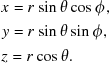 (11.37)
with the reciprocal relations
 (11.38)
The coordinate ![]() is analogous to latitude in geography, in which
is analogous to latitude in geography, in which ![]() and
and ![]() correspond to the North and South Poles, respectively. Similarly, the angle
correspond to the North and South Poles, respectively. Similarly, the angle ![]() is analogous to geographic longitude, which specifies the east or west angle with respect to the Greenwich meridian. The ranges of the spherical polar coordinates are given by:
is analogous to geographic longitude, which specifies the east or west angle with respect to the Greenwich meridian. The ranges of the spherical polar coordinates are given by:
![]()
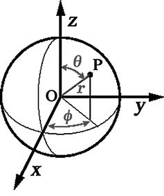
The volume element in spherical polar coordinates can be determined from the Jacobian:
 (11.39)
Therefore, a three-dimensional integral can be written
![]() (11.40)
(11.40)
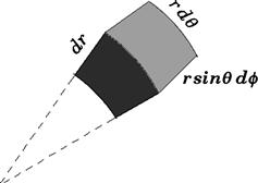
A wedge-shaped differential element of volume in spherical polar coordinates is shown in Figure 11.8.
Integration over the two polar angles gives
![]() (11.41)
(11.41)
This represents the ![]() steradians of solid angle which radiate from every point in three-dimensional space. For integration over a spherical symmetrical function
steradians of solid angle which radiate from every point in three-dimensional space. For integration over a spherical symmetrical function ![]() , independent of
, independent of ![]() and
and ![]() , (11.40) can be simplified to
, (11.40) can be simplified to
![]() (11.42)
(11.42)
This is equivalent to integration over a series of spherical shells of area ![]() and thickness dr.
and thickness dr.
Problem 11.5.1
The 1s orbital of the hydrogen atom is described by the wavefunction ![]() , where
, where ![]() is the Bohr radius. Calculate the integral of
is the Bohr radius. Calculate the integral of ![]() over all space.
over all space.
11.6 Differential Expressions
Differential quantities of the type
![]() (11.43)
(11.43)
known as Pfaff differential expressions are of central importance in thermodynamics. Two cases are to be distinguished. Eq. (11.43) is an exact differential if there exists some function ![]() for which it is the total differential; an inexact differential if there exists no function which gives (11.43) upon differentiation. If dq is exact, we can write
for which it is the total differential; an inexact differential if there exists no function which gives (11.43) upon differentiation. If dq is exact, we can write
![]() (11.44)
(11.44)
Comparing with the total differential of ![]() ,
,
![]() (11.45)
(11.45)
we can identify
![]() (11.46)
(11.46)
Note further that
![]() (11.47)
(11.47)
As discussed earlier, mixed second derivatives of well-behaved functions are independent of the order of differentiation. This leads to Euler’s reciprocity relation
![]() (11.48)
(11.48)
which is a necessary and sufficient condition for exactness of a differential expression. Note that the reciprocity relation neither requires nor identifies the function ![]() .
.
A simple example of an exact differential expression is
![]() (11.49)
(11.49)
Here ![]() and
and ![]() , so that
, so that ![]() and Euler’s condition is satisfied. It is easy to identify the function in this case as
and Euler’s condition is satisfied. It is easy to identify the function in this case as ![]() , since
, since ![]() . A differential expression for which the reciprocity test fails is
. A differential expression for which the reciprocity test fails is
![]() (11.50)
(11.50)
Here ![]() , so that dq is inexact and no function exists whose total differential equals (11.50).
, so that dq is inexact and no function exists whose total differential equals (11.50).
However, an inexact differential can be cured! An inexact differential expression ![]() with
with ![]() can be converted into an exact differential expression by use of an integrating factor
can be converted into an exact differential expression by use of an integrating factor![]() . This means that
. This means that ![]() becomes exact with
becomes exact with
![]() (11.51)
(11.51)
For example, (11.50) can be converted into an exact differential by choosing ![]() so that
so that
![]() (11.52)
(11.52)
Alternatively, ![]() converts the differential to
converts the differential to ![]() , while
, while ![]() converts it to
converts it to ![]() . In fact,
. In fact, ![]() times any function of
times any function of ![]() is also an integrating factor. An integrating factor exists for every differential expression in two variables, such as (11.43). For differential expressions in three or more variables, such as
is also an integrating factor. An integrating factor exists for every differential expression in two variables, such as (11.43). For differential expressions in three or more variables, such as
![]() (11.53)
(11.53)
an integrating factor does not always exist.
The First and Second Laws of Thermodynamics can be formulated mathematically in terms of exact differentials. Individually, dq, an increment of heat gained by a system and dw, an increment of work done on a system are represented by inexact differentials. The First Law postulates that their sum is an exact differential:
![]() (11.54)
(11.54)
which is identified with the internal energy U of the system. A mathematical statement of the Second Law is that 1/T, the reciprocal of the absolute temperature, is an integrating factor for dq in a reversible process. The exact differential
![]() (11.55)
(11.55)
defines the entropy S of the system. These powerful generalizations hold true no matter how many independent variables are necessary to specify the thermodynamic system.
Consider the special case of reversible processes on a single-component thermodynamic system. A differential element of work in expansion or compression is given by ![]() , where
, where ![]() is the pressure and V, the volume. Using (11.55), the differential of heat equals
is the pressure and V, the volume. Using (11.55), the differential of heat equals ![]() . Therefore the First Law (11.54) reduces to
. Therefore the First Law (11.54) reduces to
![]() (11.56)
(11.56)
sometimes known as the fundamental equation of thermodynamics. Remarkably, since this relation contains only functions of state, U, T, S, P, and V, it applies very generally to all thermodynamic processes—reversible and irreversible. The structure of this differential expression implies that the energy U is a natural function of S and ![]() , and identifies the coefficients
, and identifies the coefficients
![]() (11.57)
(11.57)
The independent variables in a differential expression can be changed by a Legendre tranformation. For example, to reexpress the fundamental equation in terms of S and p, rather than S and V, we define the enthalpy![]() . This satisfies the differential relation
. This satisfies the differential relation
![]() (11.58)
(11.58)
which must be the differential of the function ![]() . Analogously we can define the Helmholtz free energy
. Analogously we can define the Helmholtz free energy![]() , such that
, such that
![]() (11.59)
(11.59)
and the Gibbs free energy![]() , which satisfies
, which satisfies
![]() (11.60)
(11.60)
A Legendre transformation also connects the Lagrangian and Hamiltonian functions in classical mechanics. For a particle moving in one dimension, the Lagrangian ![]() can be written
can be written
![]() (11.61)
(11.61)
with the differential form
![]() (11.62)
(11.62)
Note that
![]() (11.63)
(11.63)
which is recognized as the momentum of the particle. The Hamiltonian is defined by the Legendre transformation
![]() (11.64)
(11.64)
This leads to
![]() (11.65)
(11.65)
which represents the total energy of the system.
Problem 11.6.2
Generalize the transformation from the Lagrangian ![]() to the Hamiltonian
to the Hamiltonian ![]() in three dimensions. The Lagrangian is given by
in three dimensions. The Lagrangian is given by
![]()
where ![]() , and
, and ![]() , the velocity vector.
, the velocity vector.
11.7 Line Integrals
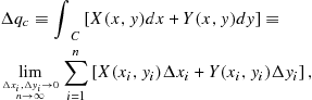
The extension of the concept of integration considered in this section involves continuous summation of a differential expression along a specified path C. For the case of two independent variables, the line integral can be defined as follows:
 (11.66)
where ![]() and
and ![]() . All the points
. All the points ![]() lie on a continuous curve C connecting
lie on a continuous curve C connecting ![]() to
to ![]() , as shown in Figure 11.9. In mechanics, the work done on a particle is equal to the line integral of the applied force along the particle’s trajectory.
, as shown in Figure 11.9. In mechanics, the work done on a particle is equal to the line integral of the applied force along the particle’s trajectory.
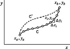
Figure 11.9 Line integral as limit of summation at points ![]() along path C between
along path C between ![]() and
and ![]() . The value of the integral along path
. The value of the integral along path ![]() will, in general, be different.
will, in general, be different.
The line integral (11.66) reduces to a Riemann integral when the path of integration is parallel to either coordinate axis. For example along the linear path ![]() , we obtain
, we obtain
![]() (11.67)
(11.67)
More generally, when the curve C can be represented by a functional relation ![]() can be eliminated from (11.66) to give
can be eliminated from (11.66) to give
![]() (11.68)
(11.68)
In general, the value of a line integral depends on the path of integration. Thus the integrals along paths C and ![]() in Figure 11.9 can give different results. However, for the special case of a line integral over an exact differential, the line integral is independent of path, its value being determined by the initial and final points. To prove this, suppose that
in Figure 11.9 can give different results. However, for the special case of a line integral over an exact differential, the line integral is independent of path, its value being determined by the initial and final points. To prove this, suppose that ![]() is an exact differential equal to the total differential of the function
is an exact differential equal to the total differential of the function ![]() . We can therefore substitute in Eq. (11.66)
. We can therefore substitute in Eq. (11.66)
![]() (11.69)
(11.69)
and
![]() (11.70)
(11.70)
neglecting terms of higher order in ![]() and
and ![]() . Accordingly,
. Accordingly,
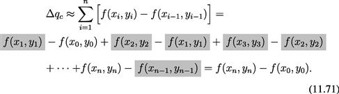
noting that all the shaded intermediate terms cancel out. In the limit ![]() , we find therefore
, we find therefore
![]() (11.72)
(11.72)
independent of the path C, just like a Riemann integral.
Of particular significance are line integrals around closed paths, in which the initial and final points coincide. For such cyclic paths, the integral sign is written ![]() . The closed curve is by convention traversed in the counterclockwise direction. If
. The closed curve is by convention traversed in the counterclockwise direction. If ![]() is an exact differential, then
is an exact differential, then
![]() (11.73)
(11.73)
for an arbitrary closed path C. (There is the additional requirement that ![]() must be analytic within the path C, with no singularities.) When
must be analytic within the path C, with no singularities.) When ![]() is inexact, the cyclic integral is, in general, different from zero. As an example, consider the integral around the rectagular closed path shown in Figure 11.10. For the two prototype examples of differential expressions
is inexact, the cyclic integral is, in general, different from zero. As an example, consider the integral around the rectagular closed path shown in Figure 11.10. For the two prototype examples of differential expressions ![]() [Eqs. (11.49) and (11.50)] we find
[Eqs. (11.49) and (11.50)] we find
![]() (11.74)
(11.74)

11.8 Green’s Theorem
A line integral around a curve C can be related to a double Riemann integral over the enclosed area S by Green’s theorem:
![]() (11.75)
(11.75)
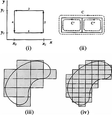
Green’s theorem can be most easily proved by following the successive steps shown in Figure 11.11. The line integral around the small rectangle in (i) gives four contributions, which can be written
 (11.76)
However,
![]() (11.77)
(11.77)
and
![]() (11.78)
(11.78)
which establishes Green’s theorem for the rectangle:
![]() (11.79)
(11.79)
This is applicable as well for the composite figure formed by two adjacent rectangles, as in (ii). Since the line integral is taken counterclockwise in both rectangles, the common side is transversed in opposite directions along paths C and ![]() , and the two contributions cancel. More rectangles can be added to build up the shaded figure in (iii). Green’s theorem remains valid when S corresponds to the shaded area and C to its zigzag perimeter. In the final step (iv), the elements of the rectangular grid are shrunken to infinitesimal size to approach the area and perimeter of an arbitrary curved figure.
, and the two contributions cancel. More rectangles can be added to build up the shaded figure in (iii). Green’s theorem remains valid when S corresponds to the shaded area and C to its zigzag perimeter. In the final step (iv), the elements of the rectangular grid are shrunken to infinitesimal size to approach the area and perimeter of an arbitrary curved figure.
By virtue of Green’s theorem, the interrelationship between differential expressions and their line integrals can be succinctly summarized. For a differential expression ![]() , any of the following statements implies the validity of the other two:
, any of the following statements implies the validity of the other two:
1. There exists a function ![]() whose total differential equals
whose total differential equals ![]() (dq is an exact differential).
(dq is an exact differential).
Problem 11.8.1
Show that the area bounded by a smooth closed curve is given by
![]()