
If we want to try a prediction of milk production in the next January, we can think in the following way: with the acquired data, we can trace the trend line and extend it until the following January. In this way, we would have a rough estimate of milk production that we should expect in the immediate future.
But tracing a trend line means tracing the regression line. The linear regression method consists of precisely identifying a line that is capable of representing point distribution in a two-dimensional plane. As is easy to imagine, if the points corresponding to the observations are near the line, then the chosen model will be able to effectively describe the link between the variables. In theory, there are an infinite number of lines that may approximate the observations. In practice, there is only one mathematical model that optimizes the representation of the data.
To fit a linear regression model, we start importing two more libraries:
import numpy
from sklearn.linear_model import LinearRegression
NumPy is the fundamental package for scientific computing with Python. It contains, among other things:
- A powerful N-dimensional array object
- Sophisticated (broadcasting) functions
- Tools for integrating C/C++ and FORTRAN code
- Useful linear algebra, Fourier transform, and random number capabilities
Besides its obvious scientific uses, NumPy can also be used as an efficient multi-dimensional container of generic data. Arbitrary datatypes can be defined. This allows NumPy to seamlessly and speedily integrate with a wide variety of databases.
sklearn is a free software machine learning library for the Python programming language. It features various classification, regression and clustering algorithms including support vector machines, random forests, gradient boosting, k-means and DBSCAN, and is designed to interoperate with the Python numerical and scientific libraries NumPy and SciPy.
We begin to prepare the data:
X = [i for i in range(0, len(data))]
X = numpy.reshape(X, (len(X), 1))
y = data.values
First, we counted the data; then we used the reshape() function to give a new shape to an array without changing its data. Finally, we inserted the time series values into the y variable. Now we can build the linear regression model:
LModel = LinearRegression()
The LinearRegression() function performs a ordinary least squares linear regression. The ordinary least squares method is an optimization technique (or regression) that allows us to find a function, represented by an optimal curve (or regression curve) that is as close as possible to a set of data. In particular, the function found must be one that minimizes the sum of squares of distances between the observed data and those of the curve that represents the function itself.
Given n points (x1, y1), (x2, y2), ... (xn, yn) in the observed population, a least squares regression line is defined as the equation line:
y=α*x+β
For which the following quantity is minimal:

This quantity represents the sum of squares of distances of each experimental datum (xi, yi) from the corresponding point on the straight line (xi, αxi+β), as shown in the following plot:

Now, we have to apply the fit method to fit the linear model:
LModel.fit(X, y)
A linear regression model basically finds the best value for the intercept and slope, which results in a line that best fits the data. To see the value of the intercept and slope calculated by the linear regression algorithm for our dataset, execute the following code:
print(LModel.intercept_,LModel.coef_)
The following results are returned:
[613.37496478] [[1.69261519]]
The first is the intercept; the second is the coefficient of the regression line. Now that we have trained our algorithm, it's time to make some predictions. To do so, we will use the whole data and see how accurately our algorithm predicts the percentage score. Remember, our scope is to locate the time series trend. To make predictions on the whole data, execute the following code:
trend = LModel.predict(X)
It is time to visualize what we have achieved:
plt.plot(y)
plt.plot(trend)
plt.show()
With this code, we first traced the time series. So we added the regression line that represents the data trend, and finally we printed the whole thing, as shown in the following graph:
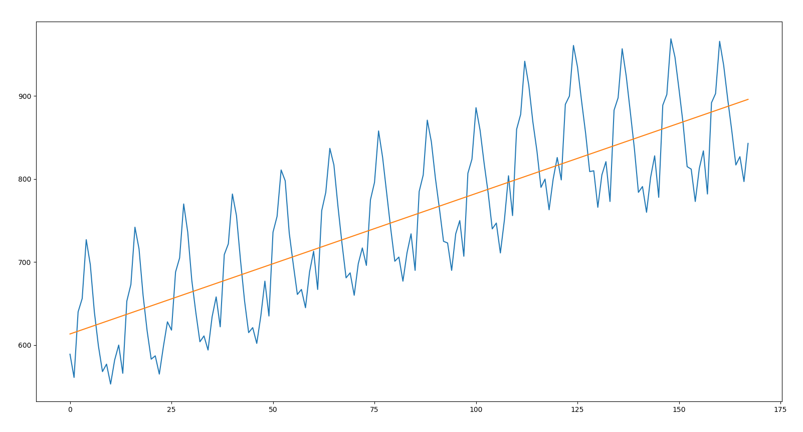
We recall that this represents a long-term monotonous trend movement, which highlights a structural evolution of the phenomenon due to causes that act in a systematic manner on the same. From the analysis of the previous figure, it is possible to note this: making a estimation of milk production in a precise period based on the line that indicates the trend of the time series can, in some cases, be disastrous. This is due to the fact that the seasonal highs and lows are at important distances from the line of regression. It is clear that it is not possible to use this line to make estimates of milk production.