2
BINARY IN ACTION

In the previous chapter we defined a computer as an electronic device that can be programmed to carry out a set of logical instructions. We then learned at a high level how everything in a computer, from the data it uses to the instructions it carries out, is stored in binary, 0s and 1s. In this chapter, I shed some light on how exactly 0s and 1s can be used to represent nearly any kind of data. We also cover how binary lends itself to logical operations.

Representing Data Digitally

So far, we’ve focused on storing numbers in binary. More specifically, we covered how to store the positive integers, sometimes called whole numbers, and zero. However, computers store all data as bits: negative numbers, fractional numbers, text, colors, images, audio, and video, to name a few. Let’s consider how various types of data might be represented using binary.

Digital Text

Let’s begin with text as our first example of how bits, 0s and 1s, can represent something other than a number. In the context of computing, text means a collection of alphanumeric and related symbols, also called characters. Text is usually used to represent words, sentences, paragraphs, and so forth. Text does not include formatting (bold, italics). For the purposes of this discussion, let’s limit our character set to the English alphabet and related characters. In computer programming, the term string is also commonly used to refer to a sequence of text characters.

Keeping that definition of text in mind, what exactly do we need to represent? We need A through Z, uppercase and lowercase, meaning A is a different symbol than a. We also want punctuation marks like commas and periods. We need a way to represent spaces. We also need digits 0 through 9. The digit requirement can be confusing; here I’m talking about including the symbols or characters that are used to represent the numbers 0 through 9, which is a different thing than storing the numbers 0 through 9.

If we add up all the unique symbols we need to represent, just described, we have around 100 characters. So, if we need to have a unique combination of bits to represent each character, how many bits do we need per character? A 6-bit number gives us 64 unique combinations, which isn’t quite enough. But a 7-bit number gives us 128 combinations, enough to represent the 100 or so characters we need. However, since computers usually work in bytes, it makes sense to just round up and use a full 8 bits, one byte, to represent each character. With a byte we can represent 256 unique characters.

So how might we go about using 8 bits to represent each character? As you may expect, there’s already a standard way of representing text in binary, and we’ll get to that in a minute. But before we do that, it’s important to understand that we can make up any scheme we want to represent each character, as long as the software running on a computer knows about our scheme. That said, some schemes are better than others for representing certain types of data. Software designers prefer schemes that make common operations easy to perform.

Imagine that you are responsible for creating your own system that represents each character as a set of bits. You might decide to assign 0b00000000 to represent character A, and 0b00000001 to represent character B, and so on. This process of translating data into a digital format is known as encoding; when you interpret that digital data, it’s known as decoding.

ASCII

Fortunately, we already have several standard ways to represent text digitally, so we don’t have to invent our own! American Standard Code for Information Interchange (ASCII) is a format that represents 128 characters using 7 bits per character, although each character is commonly stored using a full byte, 8 bits. Using 8 bits instead of 7 just means we have an extra leading bit, left as 0. ASCII handles the characters needed for English, and another standard, called Unicode, handles characters used in nearly all languages, English included. For now, let’s focus on ASCII to keep things simple. Table 2-1 shows the binary and hexadecimal values for a subset of ASCII characters. The first 32 characters aren’t shown; they are control codes such as carriage return and form feed, originally intended for controlling devices rather than storing text.

Table 2-1: ASCII Characters 0x20 Through 0x7F

Binary	Hex	Char	Binary	Hex	Char	Binary	Hex	Char
00100000	20	[Space]	01000000	40	@	01100000	60	`
00100001	21	!	01000001	41	A	01100001	61	a
00100010	22	"	01000010	42	B	01100010	62	b
00100011	23	#	01000011	43	C	01100011	63	c
00100100	24	$	01000100	44	D	01100100	64	d
00100101	25	%	01000101	45	E	01100101	65	e
00100110	26	&	01000110	46	F	01100110	66	f
00100111	27	'	01000111	47	G	01100111	67	g
00101000	28	(	01001000	48	H	01101000	68	h
00101001	29	)	01001001	49	I	01101001	69	i
00101010	2A	*	01001010	4A	J	01101010	6A	j
00101011	2B	+	01001011	4B	K	01101011	6B	k
00101100	2C	,	01001100	4C	L	01101100	6C	l
00101101	2D	-	01001101	4D	M	01101101	6D	m
00101110	2E	.	01001110	4E	N	01101110	6E	n
00101111	2F	/	01001111	4F	O	01101111	6F	o
00110000	30	0	01010000	50	P	01110000	70	p
00110001	31	1	01010001	51	Q	01110001	71	q
00110010	32	2	01010010	52	R	01110010	72	r
00110011	33	3	01010011	53	S	01110011	73	s
00110100	34	4	01010100	54	T	01110100	74	t
00110101	35	5	01010101	55	U	01110101	75	u
00110110	36	6	01010110	56	V	01110110	76	v
00110111	37	7	01010111	57	W	01110111	77	w
00111000	38	8	01011000	58	X	01111000	78	x
00111001	39	9	01011001	59	Y	01111001	79	y
00111010	3A	:	01011010	5A	Z	01111010	7A	z
00111011	3B	;	01011011	5B	[	01111011	7B	{
00111100	3C	<	01011100	5C		01111100	7C	|
00111101	3D	=	01011101	5D	]	01111101	7D	}
00111110	3E	>	01011110	5E	^	01111110	7E	~
00111111	3F	?	01011111	5F	_	01111111	7F	[Delete]

It’s fairly straightforward to represent text in a digital format. A system like ASCII maps each character, or symbol, to a unique sequence of bits. A computing device then interprets that sequence of bits and displays the appropriate symbol to the user.

Digital Colors and Images

Now that we’ve seen how to represent numbers and text in binary, let’s explore another type of data: color. Any computing device that has a color graphics display needs to have some system for describing colors. As you might expect, as with text, we already have standard ways of storing color data. We’ll get to them, but first let’s design our own system for digitally describing colors.

Let’s limit our range of colors to black, white, and shades of gray. This limited set of colors is known as grayscale. Just like we did with text, let’s begin by deciding how many unique shades of gray we want to represent. Let’s keep it simple and go with black, white, dark gray, and light gray. That’s four total grayscale colors, so how many bits do we need to represent four colors? Only 2 bits are needed. A 2-bit number can represent four unique values, since 2 raised to the power of 2 is 4.

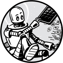
Once you’ve designed a system for representing shades of gray in binary, you can build on that approach and create your own system for describing a simple grayscale image. An image is essentially an arrangement of colors on a two-dimensional plane. Those colors are typically arranged in a grid composed of single-color squares called pixels. Here’s a simple example in Figure 2-1.

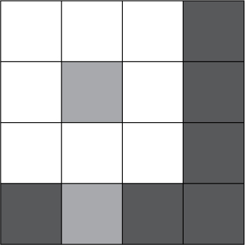
Figure 2-1: A simple image

The image in Figure 2-1 has a width of 4 pixels and a height of 4 pixels, giving it a total of 16 pixels. If you squint and use your imagination, you may see a white flower and a dark sky beyond. The image consists of only three colors: white, light gray, and dark gray.

In Exercise 2-4, in part 2, you acted like a computer program that was responsible for encoding an image into binary data. In part 3, your friend acted like a computer program that was responsible for the reverse, decoding binary data into an image. Hopefully she was able to decipher your binary data and draw a flower! If your friend pulled it off, then great, together you demonstrated how software encodes and decodes data! If things didn’t go so well, and she ended up drawing something more like a pickle than a flower, that’s okay too; you demonstrated how sometimes software has flaws, leading to unexpected results.

Approaches for Representing Colors and Images

As mentioned earlier, there are already standard approaches defined for representing colors and images in a digital manner. For grayscale images, one common approach is to use 8 bits per pixel, allowing for 256 shades of gray. Each pixel’s value typically represents the intensity of light, so 0 represents no light intensity (black) and 255 represents full intensity (white), and values in between are varying shades of gray, from dark to light. Figure 2-2 illustrates various shades of gray using an 8-bit encoding scheme.

Figure 2-2: Shades of gray represented with 8 bits, shown as binary, hex, and decimal

Representing colors beyond shades of gray works in a similar manner. Although grayscale can be represented with a single 8-bit number, an approach known as RGB uses three 8-bit numbers to represent the intensity of Red, Green, and Blue that combine to make a single color. Dedicating 8 bits to each of the three component colors means 24 bits are needed to represent the overall color.

For example, the color red is represented in RGB with all 8 red bits set to 1, and the remaining 16 bits for the other two colors set to 0. Or if you wanted to represent yellow, which is a combination of red and green, but no blue, you could set the red and green bits to all 1s and leave the blue bits as all 0s. This is illustrated in Figure 2-3.

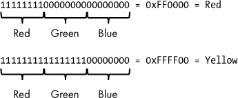
Figure 2-3: Red and yellow represented using RGB

In both the examples in Figure 2-3, the colors that are “on” are all 1s, but the RGB system allows for the red, blue, and green component colors to be partial strength as well. Each component color can vary from 00000000 (0 decimal/0 hex) to 11111111 (255 decimal/FF hex). A lower value represents a darker shade of that color, and a higher value represents a brighter shade of that color. With this flexibility of mixing colors, we can represent nearly any shade imaginable.

Not only are there standard ways of representing colors, but there are also multiple, commonly used approaches for representing an entire image. As you saw in Figure 2-1, we can construct images using a grid of pixels, with each pixel set to a particular color. Over the years, multiple image formats have been devised to do just that. A simplistic approach of representing an image is called a bitmap. Bitmap images store the RGB color data for each individual pixel. Other image formats, such as JPEG and PNG, use compression techniques to reduce the number of bytes required to store an image, as compared to a bitmap.

Interpreting Binary Data

Let’s examine one more binary value: 011000010110001001100011. What do you think it represents? If we assume it is an ASCII text string, it represents “abc.” On the other hand, perhaps it represents a 24-bit RGB color, making it a shade of gray. Or maybe it is a positive integer, in which case it is 6,382,179 in decimal. These various interpretations are illustrated in Figure 2-4.

Figure 2-4: Interpretations of 011000010110001001100011

So which is it? It can be any of these, or something else entirely. It all depends on the context in which the data is interpreted. A text editor program will assume the data is text, whereas an image viewer may assume it is the color of a pixel in an image, and a calculator may assume it is a number. Each program is written to expect data in a particular format, and so a single binary value has different meanings in various contexts.

We’ve demonstrated how binary data can be used to represent numbers, text, colors, and images. From this you can make some educated guesses about how other types of data can be stored, such as video or audio. There’s no limit on what kinds of data can be represented digitally. The digital representation isn’t always a perfect replica of the original data, but in many cases that isn’t a problem. Being able to represent anything as a sequence of 0s and 1s is enormously useful, since once we’ve built a device that works with binary data we can adapt it, through software, to deal with any kind of data!

Binary Logic

We’ve established the utility of using binary to represent data, but computers do more than simply store data. They allow us to work with data as well. With a computer’s help, we can read, edit, create, transform, share, and otherwise manipulate data. Computers give us the capability to process data in many ways using hardware that we can program to execute a sequence of simple instructions—instructions like “add two numbers together” or “check if two values are equal.” Computer processors that implement these instructions are fundamentally based on binary logic, a system for describing logical statements where variables can only be one of two values—true or false. Let’s now examine binary logic, and in the process, we’ll again see how everything in a computer comes down to 1s and 0s.

Let’s consider how binary is a natural fit for logic. Typically, when someone speaks of logic, they mean reasoning, or thinking through what is known in order to arrive at a valid conclusion. When presented with a set of facts, logic allows us to determine whether another related statement is also factual. Logic is all about truth—what is true, and what is false. Likewise, a bit can only be one of two values, 1 or 0. Therefore, a single bit can be used to represent a logical state of true (1) or false (0).

Let’s look at an example logical statement:

GIVEN a shape has four straight sides,
AND GIVEN the shape has four right angles,
I CONCLUDE that the shape is a rectangle.

This example has two conditions (four sides, four right angles) that must both be true for the conclusion to be true as well. For this kind of situation, we use the logical operator AND to join the two statements together. If either of the conditions is false, then the conclusion is false as well. I’ve expressed that same logic in Table 2-2.

Table 2-2: Logical Statement for a Rectangle

Four sides	Four right angles	Is a rectangle
False	False	False
False	True	False
True	False	False
True	True	True

Using Table 2-2, we can interpret each row as follows:

1. If the shape does not have four sides and does not have four right angles, it is not a rectangle.
2. If the shape does not have four sides and does have four right angles, it is not a rectangle.
3. If the shape does have four sides and does not have four right angles, it is not a rectangle.
4. If the shape does have four sides and does have four right angles, it is a rectangle!

This type of table is known as a truth table: a table that shows all the possible combinations of conditions (inputs) and their logical conclusions (outputs). Table 2-2 was written specifically for our statement about a rectangle, but really, the same table applies to any logical statement joined with AND.

In Table 2-3, I’ve made this table more generic, using A and B to represent our two input conditions, and Output to represent the logical result. Specifically, for this table Output is the result of A AND B.

Table 2-3: AND Truth Table (Using True and False)

A	B	Output
False	False	False
False	True	False
True	False	False
True	True	True

In Table 2-4, I’ve made one more modification to our table. Since this book is about computing, I’ve represented false as 0 and true as 1, just like computers do.

Table 2-4: AND Truth Table

A	B	Output
0	0	0
0	1	0
1	0	0
1	1	1

Table 2-4 is the standard form of an AND truth table when you’re dealing with digital systems that use 0 and 1. Computer engineers use such tables to express how components will behave when they’re presented with a certain set of inputs. Now let’s examine how this works with other logical operators and more complex logical statements.

Let’s say you work at a shop that gives a discount to only two types of customers: children and people wearing sunglasses. No one else is eligible for a discount. If you wanted to state the store’s policy as a logical expression, you could say the following:

GIVEN the customer is a child,
OR GIVEN the customer is wearing sunglasses,
I CONCLUDE that the customer is eligible for a discount.

Here we have two conditions (child, wearing sunglasses) where at least one condition must be true for the conclusion to be true. In this situation we use the logical operator OR to join the two statements together. If either condition is true, then the conclusion is true as well. We can express this as a truth table, as shown in Table 2-5.

Table 2-5: OR Truth Table

A	B	Output
0	0	0
0	1	1
1	0	1
1	1	1

By observing the inputs and output in Table 2-5, we can quickly see that a discount will be given (Output = 1) when either the customer is a child (A = 1) or the customer is wearing sunglasses (B = 1). Note that the input column values for A and B are exactly the same for both Table 2-4 and Table 2-5. This makes sense, because both tables have two inputs and thus the same possible set of input combinations. What differs is the Output column.

Let’s combine AND with OR in a more complex logical statement. For the purposes of this example, assume that I go to the beach every day that is sunny and warm, and also assume that I go to the beach every year on my birthday. In fact, I only and always go to the beach under these specific circumstances—my wife says I’m overly stubborn in this way. Combining those ideas gives us the following logical statement:

GIVEN it is sunny AND GIVEN it is warm,
OR GIVEN it is my birthday,
I CONCLUDE that I am going to the beach.

Let’s label our input conditions, then write a truth table for this expression.

Condition A   It is sunny.

Condition B   It is warm.

Condition C   It is my birthday.

Our logical expression will look like this:

(A AND B) OR C

Just like in an algebraic expression, the parentheses around A AND B mean that part of the expression should be evaluated first. Table 2-6 gives us a truth table for this logical expression.

Table 2-6: (A AND B) OR C Truth Table

A	B	C	Output
0	0	0	0
0	0	1	1
0	1	0	0
0	1	1	1
1	0	0	0
1	0	1	1
1	1	0	1
1	1	1	1

Table 2-6 is a bit more complex than a simple AND truth table, but it’s still understandable. The table format makes it easy to look up a certain condition and see the outcome. For example, the third row tells us that if A = 0 (it is not sunny), B = 1 (it is warm), C = 0 (it is not my birthday), then Output = 0 (I’m not going to the beach today).

This kind of logic is something that computers regularly need to handle. In fact, as mentioned earlier, the fundamental capabilities of a computer distill down to sets of logical operations. Although a simple AND operator may seem far removed from the capabilities of a smartphone or laptop, these logical operators serve as the conceptual building blocks of all digital computers.

Besides AND and OR, several other common logical operators are used in the design of digital systems. I cover each operator in the following pages and provide a truth table for each. We use these again in Chapter 4 on digital circuits.

The logical operator NOT is just what it sounds like, the output is the opposite of the input condition. That is, if A is true, then the output is not true, and vice versa. As you can see in Table 2-8, NOT only takes a single input, rather than two inputs.

Table 2-8: NOT Truth Table

A	Output
0	1
1	0

The operator NAND means NOT AND, so the output is the reverse of AND. If both inputs are true, the result is false. Otherwise, the result is true. This is shown in Table 2-9.

Table 2-9: NAND Truth Table

A	B	Output
0	0	1
0	1	1
1	0	1
1	1	0

The NOR operator means NOT OR, so the output is the reverse of OR. If both inputs are false, the result is true. Otherwise, the result is false. Table 2-10 shows this as a truth table.

Table 2-10: NOR Truth Table

A	B	Output
0	0	1
0	1	0
1	0	0
1	1	0

XOR is Exclusive OR, meaning that only a single (exclusive) input can be true for the result to be true. That is, the output is true if only A is true or only B is true, while the output is false if both inputs are true. This is detailed in Table 2-11.

Table 2-11: XOR Truth Table

A	B	Output
0	0	0
0	1	1
1	0	1
1	1	0

The study of logical functions of two-value variables (true or false) is known as Boolean algebra or Boolean logic. George Boole described this approach to logic in the 1800s, well before the advent of the digital computer. His work proved to be foundational to the development of digital electronics, including the computer.

Summary

In this chapter, we covered how binary is used to represent both data and logical states. You learned how 0s and 1s can be used to represent nearly any kind of data. We looked at text, colors, and images as examples of data in a binary format. You were introduced to various logical operators, such as AND and OR, and you learned about using truth tables to express a logical statement. Understanding this is important because the complex processors found in today’s computers are based on an intricate system of logic.

We return to the topic of binary when we discuss digital circuits in Chapter 4, but first, to prepare you for that topic, we will take a detour in Chapter 3 to cover the fundamentals of electrical circuits. We’ll explore the laws of electricity, see how electrical circuits work, and get familiar with some basic components found in many circuits. You’ll even have an opportunity to build your own circuits!