CHAPTER 3

Understanding the Price Sensitivity of Buyers

The law of demand asserts that as the price of a good rises, the quantity demanded decreases and vice versa. Another key element of demand theory that is critical to price-setting is the price elasticity of demand. The price elasticity of demand refers to the responsiveness of the quantity demanded to price changes. Drivers inevitably grumble about rising gasoline prices, and for good reason. Many individuals regard driving as a necessity because they simply live too far from work, school, or other valued destinations to walk or ride a bike. Moreover, their cars only run on gas: they can’t pump lemonade into their tanks if the price of gas becomes too costly. But consumers are less likely to complain about the rising price of frozen yogurt, and for two reasons. First, frozen yogurt is unlikely to be viewed as a necessity. If the consumer thinks the price is too high, she can simply do without. Moreover, ice cream and frozen custard are reasonably close substitutes for frozen yogurt. Therefore, if the price of frozen yogurt rises, the consumer can purchase the substitute.

Let’s illustrate the concept of price elasticity graphically. Figure 3.1 shows the demand curves for gasoline and frozen yogurt. Note that whereas the law of demand holds in both cases, a given increase in the price leads to a larger decrease in the quantity of frozen yogurt demanded relative to the decline in the quantity of gasoline demanded. When the quantity demanded of a given product is relatively responsive to price changes (i.e. frozen yogurt), we say that good has a relatively elastic demand. When the quantity demanded of a good is not very responsive to price changes (i.e., gasoline), we say the good has a relatively inelastic demand.

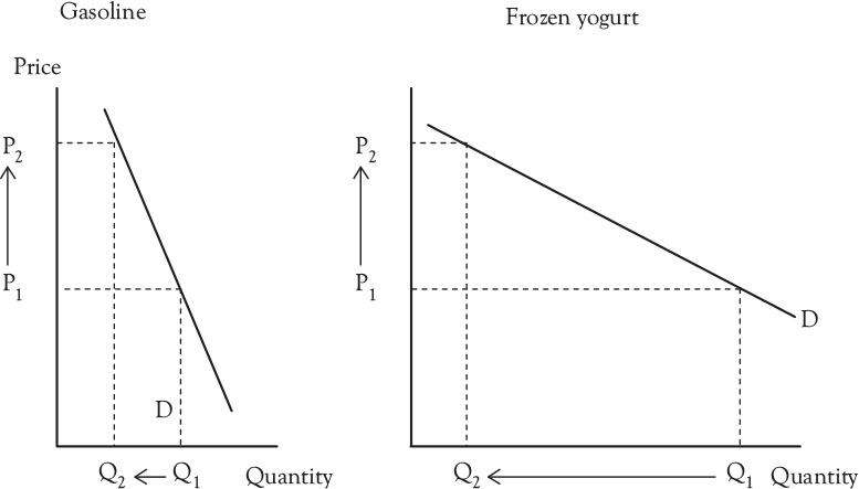
Figure 3.1. Graphical representation of price elasticity.

What determines price elasticity? We have already covered two determinants. The first determinant is whether the good is a luxury or a necessity. Clearly, if a good is considered to be a luxury, the prospective buyer may choose not to buy it if the price is too high. This is why the travel industry often suffers during recessions. Families are less likely to go on a vacation if one or more of the parents is unemployed or fears losing his job. If the product is viewed as a necessity, on the other hand, the consumer may have no choice but to continue to buy the good.

Another determinant is the availability of substitutes. Consumers look to minimize the opportunity cost of making a purchase. When the price of a good rises, they look for cheaper substitutes. Thus, when the price of frozen yogurt rises, they can substitute into ice cream, whereas the drivers cannot opt for cheaper substitutes when the price of gasoline rises.

This is why gasoline is a frequent government target for taxation. In 1980, the federal gasoline tax was 4 cents per gallon. By 1993, the tax had risen to its current level of 18.4 cents per gallon. And this is only the federal tax. Each state has its own tax, ranging from roughly 10 to 40 cents per gallon.1 Gasoline is a target for taxation because as a necessity with no viable substitutes, consumers cannot cut back significantly on their gasoline consumption when prices rise.

Another determinant of price elasticity that relates to the availability of substitutes is the definition of the market. For example, whereas consumers may view the demand for gasoline to be relatively inelastic, the same cannot be said for the gasoline sold at the gas station on the corner of First and Main. Clearly, whereas consumers have few alternatives when the price of gasoline rises, they can easily substitute away from the gasoline sold at a specific station by purchasing gas from a competing station. Thus, whereas the demand for gasoline may be inelastic, the demand for gas sold by a specific retailer is highly elastic.

Another determinant of price elasticity is the price of the good as a percentage of the consumer’s budget. The National Association for Convenience Stores reported an average gross margin of nearly 47% on warehouse-delivered snack foods at convenience stores in 2008.2 This should not come as a surprise to consumers. A candy bar that might cost $0.50 at a supermarket may cost $0.75 (50% more) at a convenience store. Why? Undoubtedly, consumers do not make the trip to the convenience store to buy snack foods. In most cases, they enter the store to finalize a gasoline purchase. In deciding whether to buy the candy bar, the consumer is well aware that a better price can be had at a supermarket. But even if the candy bar is cheaper at the supermarket, the opportunity cost of buying it at the convenience store is fairly low, particularly when one considers the time involved in finding a better price. Therefore, we would expect consumers to be relatively price inelastic when it comes to goods that are relatively inexpensive.

Although consumers may claim that they’re willing to pay the additional 50% for “convenience,” the rationale doesn’t really hold up to scrutiny. Suppose a “convenient” auto dealer was selling a new car for $30,000 whereas a competing dealer on the other side of town was offering the identical car for $20,000. Would the consumer be willing to pay the additional 50% for the convenience? Clearly, the difference between paying 50% more for a candy bar as compared to 50% more for a new car is the opportunity cost of the purchase. Regardless of whether the consumer buys the car at the convenient dealership or the one across town, the opportunity cost of the purchase is sizable. Consequently, the higher the price as a percentage of the consumer’s budget, the more price sensitive the consumer.

The final determinant of price elasticity is the time the consumer has to make a purchase. Consider an extreme case. The National Weather Service reports that a hurricane is imminent. When that occurs, coastal residents are in a rush to buy plywood hurricane shutters, install them quickly, and drive inland before the storm makes landfall. Under less trying circumstances, these same consumers would shop around for an acceptable price. With the hurricane due to arrive in a matter of hours, consumers have minimal opportunity to compare prices and may feel compelled to make a hasty purchase. Clearly, this gives a great deal more market power to the supplier of plywood, whose price need not be as competitive as it might have been during less urgent periods.

The importance of time as a determinant of price sensitivity should not be underestimated by firms. Because the price of a good represents opportunity cost, buyers constantly seek ways to minimize the opportunity cost of a purchase. Firms that foolishly believe they have the advantage over consumers will eventually find that buyers found a way to lower their opportunity costs. When the price of gas increased by $0.86/gallon between the spring of 2010 and 2011, both Toyota and Honda reported significant increases in Prius and Insight sales.3 Clearly, most consumers are not in a position to buy a new car when gas prices rise. However, if fuel prices remain high, over time, consumers will look seriously at hybrids when they need a new vehicle. In summary, then, the longer the time the consumer has to make a purchase decision, the more elastic the demand for the good.

How can knowledge of price elasticity help a firm make better pricing decisions? To begin with, we need to find a way to measure price elasticity. Because the law of demand holds regardless of whether the good has an elastic or inelastic demand, how do we distinguish one from the other? Because price elasticity refers to the responsiveness of the quantity demanded to price changes, the degree of responsiveness can be measured. Economists measure price elasticity as

EP = % change in quantity purchased/% change in price

In measuring price elasticity, note that “quantity purchased” is used instead of “quantity demanded.” Although the intent is to equate the two, this may not always be the case. If the firm stocks out of an item, the quantity demanded may exceed the quantity purchased. For firms trying to measure price elasticity, this is an important consideration. If the quantity demanded exceeds the quantity purchased due to stockouts, the results may delude managers into thinking consumers are less price sensitive than they actually are.

Because the law of demand suggests that the quantity demanded decreases as prices rise, EP is negative. The convention among many economists is to ignore the negative sign. In terms of measuring price elasticity, economists define “elastic” as any situation in which the percentage change in the quantity demanded exceeds the percentage change in the price. Based on the equation, then, if the good has a relatively elastic demand, the elasticity coefficient will be greater than one. For example, an elasticity coefficient of 2.5 means that each 1% change in the price leads to a 2.5% change in the quantity demanded. “Inelastic demand” is just the reverse: economists say that a good has a relatively inelastic demand if the percentage change in the quantity demanded is less than the percentage change in the price. In such cases, the elasticity coefficient will be less than one. For instance, if the elasticity coefficient is equal to 0.4, a 1% change in the price leads to a 0.4% change in the quantity demanded. If the percentage change in the quantity demanded is equal to the percentage change in the price (i.e. a 10% price increase leads to a 10% decrease in the quantity demanded), the good is exhibiting unitary elasticity. The definitions are summarized in Table 3.1.

The coefficient is more precisely measured as

Note that the respective denominators in calculating percentage changes are the average of the two quantities (or prices) rather than the original quantity (or price). This is to assure that the coefficient corresponding to a given price change along a demand curve will be the same regardless of whether the price increases or decreases. For example, suppose a firm increases the price from 5 to $11, and as a result, the quantity demanded decreases from six to two units. If the percentage change in the price was measured as the change in the price divided by the original price, the percentage change would be equal to 120%. If, on the other hand, the price decreased from 11 to $5, the percentage change in the price would be equal to 54.5%. By dividing the price change by the average of the two prices, the percentage change will be the same regardless of whether the original price was $5 or $11. This assures that the calculated price elasticity coefficient will be the same regardless of whether the price increases or decreases.

When calculating the price elasticity of demand, firms should be cognizant of the fact that the two price/quantity combinations may not lie on the same demand curve. Figure 3.2 illustrates the problem that may arise. The graph on the left shows two price/quantity combinations. When using the numbers to calculate the price elasticity of demand, the firm assumes they lie on the same demand curve. The graph on the right shows another possibility. One of the other determinants of demand (i.e. the price of substitutes) may have changed, causing the demand curve to shift. If the price/quantity combinations lie on different demand curves, the elasticity coefficient will be biased and could provide misleading pricing implications. One should note that the scenario on the right is quite likely to be the case. Managers usually do not change prices randomly. More often than not, the price change was motivated by a change in a factor that can shift a demand curve, such as the price charged by competing firms. Later in this text, when we discuss dynamic pricing and e-commerce, we will see opportunities for firms to obtain more accurate measures of price elasticity.4

Figure 3.2. Incorrect inference of elasticity.

The relationship between price elasticity and revenue is important. For example, suppose a firm raises its price from 5 to $10 and the quantity demanded falls from 100 to 60 units. In this case, raising the price caused the firm’s revenue to increase from 500 to $600. Suppose, however, that in response to the price increase, the quantity demanded falls from 100 to 40 units. In this circumstance, the price increase caused revenues to fall from 500 to $400. Figure 3.3 illustrates the distinction. Note that the demand curve that corresponds to the decrease in revenues is more elastic than the demand curve that is associated with an increase in revenues.

Figure 3.3. Elasticity and revenue.

When we reflect on the definitions of elastic and inelastic in Table 3.1, the relationship between elasticity and revenue should become fairly obvious. We define demand as “elastic” if the percentage change in quantity exceeds the percentage change in price. Hence, for example, if the price rises by 10%, the quantity demanded will fall by more than 10%, which implies that revenue will decrease. If, on the other hand, the price declines by 10%, the quantity demanded will rise by more than 10%. This suggests that revenues will increase in response to the price cut. In general, therefore, when the demand is elastic, price and revenue will move in opposite directions.

If demand is relatively inelastic, the percentage change in the quantity demanded will be less than the percentage change in the price. Thus, if the price rises by 10%, the quantity demanded will fall by less than 10%, causing revenue to rise. If the price falls by 10%, the quantity demanded will rise by less than 10%, leading to a decrease in revenue. If demand is inelastic, therefore, price and revenue will move in the same direction.

Finally, if demand is unitary, a given percentage change in the price will lead to an identical percentage change in the quantity demanded. For example, a 10% price hike will lead to a 10% decline in the quantity demanded. The two percentage changes cancel out, causing revenues to remain the same. Table 3.2 summarizes the relationship between elasticity and revenue.

Although many persons (economists included) tend to label a good as having either an elastic demand for an inelastic demand, the elasticity depends on the price. If we examine the demand schedule in Table 3.3 and calculate the price elasticity of demand between each pair of prices, the results are illuminating.

Table 3.3. Price Elasticities Along the Demand Curve

As Table 3.3 indicates, the price elasticity of demand is not constant across all prices. Between $3 and $5, demand is inelastic. Between $5 and $6, demand is unitary, and demand is elastic for prices above $6. We can also see that as we move up the demand curve, the coefficient becomes increasingly elastic.

This revelation should not be too surprising. We used snack foods at a convenience store to illustrate why the price of snack foods could be 50% higher than at a supermarket without causing sales to suffer dramatically. Let’s assume that the manager of the store increased the price of a candy bar from $0.50 to $0.75. Although the number of candy bars sold decreased after the price hike, revenues increased. This would indicate that the candy bars had an inelastic demand. The manager would be foolish to believe that candy bars would have an inelastic demand at all prices. If consumers were relatively insensitive to candy bar prices, and price increases were inevitably accompanied by rising revenue, then the manager would think that charging $25 for a candy bar would yield far greater revenues than $0.75. Clearly, the store would be hard-pressed to sell any candy bars at a price of $25. It stands to reason, then, that somewhere between $0.75 and $25, the demand goes from being inelastic to elastic.

Let’s see how the relationship between elasticity and the demand curve affects pricing. Theory suggests that demand tends to be relatively inelastic at lower prices, becomes unitary at a higher price, and eventually becomes elastic at even higher prices. Earlier, we stated that if the current price is in the inelastic portion of a demand curve, an increase in the price will cause revenues to rise. On the other hand, if the current price is the in elastic section of the demand curve, decreasing the price will cause revenues to rise. Taken together, this implies that the firm will maximize revenues by setting its price in the unitary section of the demand curve. This is shown in Figure 3.4. As the price moves toward P*, revenues rise. Total revenues are maximized by setting the price in the unitary section of the demand curve. At that price, Q* units are demanded.

Figure 3.4. Elasticity and the revenue-maximizing price.