CHAPTER 1
Bonds: It′s All About Discounting
Before we delve into all the good stuff (swaps and options), let us review some fixed income basics.
TIME VALUE OF MONEY: FUTURE VALUE, PRESENT VALUE
Following the classical fixed income gospels, we remember that the Future Value, FV, on a horizon date of an investment PV at an annual interest rate of r , compounded m times a year, for N whole compounding periods is
FV = PV(1+r/m)N
For example, if m = 1, we have annual compounding FV = PV(1 + r )N, and N is the number of years until the future horizon date. If m = 2, we have semiannual compounding (standard for U.S. Treasury securities) FV = PV(1 + r /2)N, and N = 2T is the number of whole semiannual periods until the horizon date (T years from now).
The above formula can be easily generalized to incorporate horizon dates that are not a whole number of compounding periods away. We compute T as the number of years between the investment date and the horizon date, according to some day count basis, and come up with:
FV = PV(1 + r/m)Tm
From college math courses, we recall that as you increase the compounding frequency, the above, in the limit, becomes and r is then referred to as the continuous compounding rate.
An alternative to using compounded rates is to use simple or noncompounding interest rates:
FV = PV(1 + r T)
where T is the number of years (can be fractional) to the horizon date. Simple interest rates are usually used for Money Market instruments, that is, with maturity less than 1 year.
In order to compute how much money needs to be invested today at interest rate r , compounded m times a year, for T years to get FV at maturity, one simply inverts the above equation to come up with Present Value, PV: and in the limit:
By setting FV to 1, PV becomes today′s price of unit currency to be received at time T, that is, present value of $1, and we will denote it by Discount Factor, D:
This would be price of a security that returns unit dollar at maturity (T years from now), that is, the price of a T-maturity zero-coupon bond, and provides an (implicit) yield r , compounded m times a year.
Note that while interest rates r can be quoted in different ways, the actual investment ( PV dollars in, FV dollars out) remains the same. In order to compare different investments, one would need to compare them using the same metric, that is, interest rates with the same quote convention. However, in order to value investments, all we need are discount factors.
Discount factors are the fundamental building blocks for valuing fixed income securities. Given a series of known cash flows (C1,...,CN) to be received at various times (T1 , . . . , TN) in the future, if we know the discount factor D(Ti ) for each payment date Ti , then today′s value of this package is:

PRICE-YIELD FORMULA
For example, today′s price P of a T-year bond paying an annualized coupon rate C, m times a year (so N = T × m payments left) is

The standard bond pricing formula is based on Flat Yield assumption: it assumes that there is a single interest rate called Yield-to-Maturity (YTM) y applicable for all cash flows of the bond, regardless of how far the payment date is. With this assumption, D(Ti ) = 1/(1 + y/m)i , and we get the classical bond pricing formula:

The above formula is for when there are N = T × m whole future coupon periods left. For a bond in the middle of a coupon period, the discount factors get modified as D(Ti ) = 1/(1 + y/m)i -w where w measures the accrued fraction (measured using some day-count convention: Act/Act, Act/365, . . .) of the current coupon period: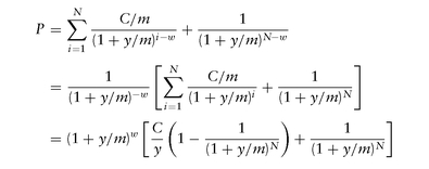

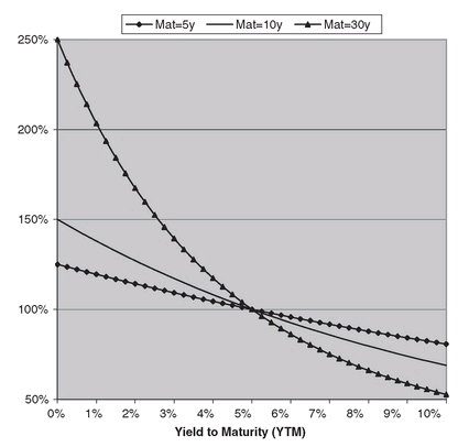
The above formula is the Dirty Price of a bond, that is, how much cash is needed in order to purchase this bond. One needs to always remember that dirty price of a bond is the discounted value of its remaining cash flows. The standard price/yield formulae simply express this via assuming a flat yield and expressing all discount factors as a function of this (hypothetical) yield y. Figure 1.1 shows the graph of Price as a function of YTM. As can be seen, when yield equals the coupon rate, the price of the bond is Par (100%). Also, longer-maturity bonds exhibit a higher curvature (convexity) in their price-yield relationship.
FIGURE 1.1 Price-Yield Graph for a 5% Semiannual Coupon Bond
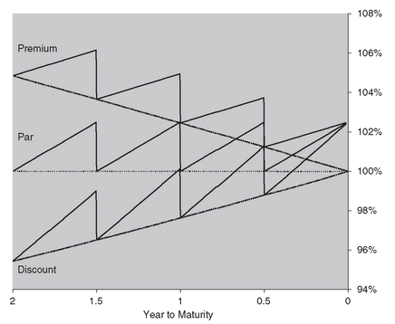
The graph of a dirty price of a bond versus time to maturity T is discontinuous, with drops (equal to paid coupon) on coupon payment dates. This makes sense, since the present value of remaining cash flows should drop when there is one less coupon. For bond traders focused on quoted price of a bond, this drop in price (while real in terms of PV of remaining cash flows) is artificial in terms of worthiness/value of a bond, and they prefer a smoother measure. By subtracting the accrued interest, wC/m from the dirty price, one arrives at the Clean/Quoted Price:

Note that when coupon rate equals yield, C = y, the term in the square brackets becomes 1, and the formula simplifies to
On coupon payment dates the accrued fraction w equals zero, and the price is par: P = 1 = 100%. In between coupon payment dates, even when C = y, the price is not exactly par. This is because the above formula is based on the Street Convention where fractional periods are adjusted using the formula suggested by compounded interest rates: 1/(1 + y/m)-w = (1 + y/m)w . If instead, we had used simple interest rates for first period, we would get the clean price using the Treasury Convention (TC): and then the price of a bond when C = y would be par (100%) at all times.

Figure 1.2 shows the evolution of the clean and dirty prices for a 2y 5% semiannual coupon bond as we get closer to maturity while holding yields constant for 3 yield scenarios: y = 7.5% leading to a Premium bond (C < y), y = 2.5% leading to a Discount bond (C > y), and y = 5% leading to a par (C = y) bond. Notice the Pull-To-Par Effect for the bond regardless of the assumed yield scenario: A discount bond gets pulled up to par, while a premium bond gets pulled down to par.
In order to flesh out the calculation details, for the remainder of the chapter, we will focus on the 2y U.S. Treasury note issued on 1-Oct-2007, with CUSIP (Committee on Uniform Security Identification Procedures) number 912828HD5, shown in Table 1.1. From Announcement date till Auction date, these 2-year notes will be considered When-Issued (WI) and trade based on yield since the coupon rate is only known at Auction time. After the auction they start trading based on price, and become the current 2y-notes, replacing the old 2y-note. Until the Issue Date, they will have a forward settlement date of Mon 1-Oct-2007, and thereafter they will have a T + 1 settlement date. The 4 coupon dates are: 31-Mar-2008, 30-Sep-2008, 31-Mar-2009, and final coupon and redemption on 30-Sep-2009. Note that U.S. treasury securities follow month-end convention, so if the maturity is at month-end, then the (assumed) coupon dates are also at month-end (March-31st, rather than March-30th).
FIGURE 1.2 Clean/Dirty Price Evolution for a 2y 5% Semiannual Coupon Bond in Unchanging Yield Scenarios
Example 1. On Tue, 2-Oct-2007, the current 2y U.S. Treasury (CT2 from now on) is trading at clean price of 100-02+ for (T+1) settlement date of Wed 3-Oct-2007:
PClean = (100 + 2.5/32)/100 = 100.078125% = 1.00078125
TABLE 1.1 Current U.S. 2y Treasury Note for Oct 2007

Although this bond′s issue date is Mon, 1-Oct-2007, it starts accruing interest (dated date) on Sun, 30-Sep-2007, and hence has 3 days of accrued interest on settlement date. U.S. Treasury securities use the ″Actual/Actual″ convention for fractional first periods and accrued interest:

Its accrued interest is then (.04/2) × (3/183) and the dirty price is:
Its semiannual yield (3.95866%) is computed by backing out (trial and error, or Newton-Raphson root-search method) the y that solves: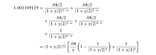

If you bought $50M face/principal of this treasury on 2-Oct-2007, then you need to pay $50,055,455.94 (= 50,000,000 × 1.001109119) to seller on 3-Oct-2007 by 3 p.m. (before the Fed-Wire closes).
True Yield
The standard bond price formula assumes that coupons are paid on specific dates, even if they are holidays. In reality, a coupon is paid on the next good business day after the assumed coupon date. Since one is paying the same amount up front, but getting the coupons later, the standard yield backed out from the bond equation potentially overstates the yield. This overstatement is more relevant for short-term bonds (sometimes referred to as short coupons), say with maturity less than 2 years, and especially when the maturity date falls on a holiday, and can be as high as a few basis points. True yield (sometimes referred to as yield adjusted for bad days) is the typically lowered yield when actual payment dates are taken into consideration. The usual formula used to back out the true yield is: where
where and Ti is the i -th true (holiday-adjusted) future payment date. Note that this replaces the exponent term for the i -th cash flow from i - w to ti , and can lead to a potentially different yield, even if all nominal payment dates are good business days. For example, for the CT2 in Example 1, even though all its nominal coupon dates fall on good business days, the True Yield using the above formula gives 3.95316% versus 3.95866% using the standard formula. As such, the above formula should mainly be used to back out the true yield adjustment.


Zero-Coupon Bonds
Treasuries can be stripped into principal (P-strip) and coupon strips (C-strip) to come up with single cash flows. One can buy these as zero-coupon bonds by paying an up-front fee (quoted price) and receiving the principal at maturity. Their yield is quoted using the standard bond equation, but with the coupon set to zero: where N is the number of hypothetical coupon periods left if the bond was paying periodic (m coupons per year) coupons, and w is the hypothetical accrued fraction. Similar to coupon bonds, we can also compute the true yield of zeros.

PV01, PVBP, CONVEXITY
Much space is wasted in the bond gospels on Macaulay Duration (sometimes abbreviated to Duration): ″In 1938, Frederick Macaulay constructed a measure. . . . In practice, nobody cares about Macaulay Duration! All we care about is the price sensitivity to changes in interest rates, that is, the derivative of the PV to yields/rates. It is the standard to consider price changes due to 1 basis-point (bp, 0.0001 = 1% of 1%) move in yields/rates, giving rise to PV01: present value of 1 basis-point increase in interest rates, sometimes called risk, or DV01 for dollar-centric folks. For a bond,
In Bond-land, PV01 is defined as the negative of the previous equation, so that a positive PV01 signifies a long position in the bond. We will stay with the true definition for the rest of the book, so a positive PV01 implies one is short the market.
Since accrued interest does not depend on yield y, the P in the above can either be the dirty or the clean price of a bond. A little bit of algebra gets us

Modified Duration is defined as the percentage change in bond price, that is, and has unit of years. While it makes sense for bonds, since swaps can have zero PV, it does not extend to swaps, swaptions, . . . , and that′s why we will stay with PV01.
A concept similar to PV01, but not identical to it is PVBP : Present value of 1 bp. This is the change in the price due to changing the coupon rate by 1 bp:

Since PVBP is the change in price, it is equivalent to PV′ing a 1 bp per annum annuity, paid m times a year, it is also called the Annuity Formula:

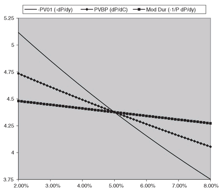
For par bonds (C = y), receiving 1 bp extra in coupon is almost equivalent to yields dropping by 1 bp, and that′s why PV01 and PVBP are (wrongly) used interchangeably in practice. For nonpar bonds, the difference can be significant, see Figure 1.3, and the appropriate formula should be used depending on the application.
FIGURE 1.3 PV01, PVBP, Modified Duration for a 5y, 5% Semiannual Coupon Bond
The convexity of a bond is a measure of the curvature of the price-yield graph, and is defined as that is, the rate of change of PV01:

PV01 and convexity can be used via a Taylor Series expansion (see Appendix A) to estimate the price change due to a small change (Δy) in yields:

In practice, one is primarily interested in the PV01, ignoring the convexity effect except for long maturity bonds, or for large rate movements. Using only the first order term in the Taylor series expansion, one gets
where Δy is expressed in basis points. The change in price, Δ P , is usually expressed in cents, that is, units of 1/10,000, or for a principal of $100 = 10,000 cents. For example, when holding a $1,000,000 face of a security, and the price changes by 5 cents, one has made $1,000,000 × 5 × 0.0001 = $500.
ΔP = P (y + Δy) - P (y) ≈ P V01 × Δy
For U.S. Treasuries, units of 1/32 of 1% (1/3200) (also called treasury ticks, or ticks for short) are usually used. In this case, when holding a $1,000,000 face of a bond, and the price moves by 1 tick, one has made $1,000,000 × 1 × (1/3200) = $312.50 = 3.125 cents. Therefore, each U.S. Treasury tick (1/32 of 1%) equals 3.125 cents.
Since we will be dealing with interest rate derivatives later, we will stay with cents, sometimes called bp′s upfront, or just bp′s. Using the previous first order approximation, one can relate the changes in yields to
TABLE 1.2 U.S. Treasury Currents for 3-Oct-2007 Settlement

P&L: Each 1 bp change in yields translates to approximately PV01 cents change in value.
Table 1.2 shows an example of PV01s and convexities of benchmark U.S. Treasuries.
Example 2. Continuing with Example 1, let us compute the above sensitivity measures for U.S. CT2 trading at 100-02+ (y = 3.95866%) for settlement on 3-Oct-2007 with dirty price of 100.1109119%. Using the previous formulae (N = 4, w = 3/183, C = .04), we get: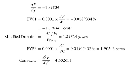

We can estimate the price change due to a small, say 10 bp, change in yields: leading to an estimate of P (y + 10 bp) = 99.88852049%. Compared to actual P (y + 10 bp) = 99.88852026%, we see that the difference is quite small (0.0007% of 1/32nd, or $0.22 for $100M face!).

PV01 is the basic measure of market risk, either for outright purchase and sale of U.S. treasuries, or for trades based on the slope of the yield curve.
Example 3. Yield Curve Trade Using prices in Table 1.2, we observe that the 2′s-10′s curve is trading at 46.35 bp (= 4.42213% - 3.95866%), which a trader might feel is too flat compared to their historical relationship. The trader can express a yield curve steepening view by buying CT2 and selling CT10 in PV01-equal amounts, that is, 4.2413 (= 8.050/1.898) units of CT2 for each unit of CT10. For example, if one buys $424.13M CT2 versus selling $100M of CT10, one is long a spread-PV01 risk of $80,500 (= $100M × 8.050 × 0.0001) per each 1 bp steepening of 2′s-10′s treasury yield curve.
Another common trade is a butterfly trade which is a way of expressing a view on the difference between slopes of the yield curve at different points, that is, on the curvature of the yield curve. For example, if one feels that 2′s/5′s is too flat compared to 5′s/10′s (5-year yields are too low in relationship to 2y, 10y yields), one can buy a 2-5-10 butterfly by buying CT2, selling CT5, and buying CT10 so that each spread leg (CT2-CT5, CT5-CT10) is PV01-equivalent.
Example 4. Butterfly Trade Using prices in Table 1.2, the 2-5-10 butterfly is trading at
which a trader might think is too low compared to history. A simple trade would be to buy the butterfly by buying the 2′s-5′s curve and selling 5′s-10′s curve in equal spread-PV01 amounts: buy N1 CT2 versus selling N2 CT5 (2′s-5′s curve), while simultaneously buying N2 CT5 versus buying N3 CT10 (5′s-10′s curve), so that
-21.6 bp = (4.42213% - 4.08233%) - (4.08233% - 3.95866%)
N2/N1 = P V01(2y)/P V01(5y)
N2/N3 = P V01(10y)/P V01(5y)
N2/N3 = P V01(10y)/P V01(5y)
For example, for a $100M sale of CT5, one has to buy $118.38M CT2 and $27.92M CT10 for an equal-weight butterfly trade.
A more common trade is to volatility-weight each curve leg. For example, if a regression analysis shows that for each 1 bp movement in 2′s-5′s, there is typically a 0.8p movement in 5′s-10′s, then one would weight the butterfly so that
that is, one has to overweight the 5′s-10′s leg due to its lower volatility, resulting in purchase of $105.23M CT2 and $31.02M CT10 for a sale of $100M CT5.
P V01(2′s - 5′s)/ P V01(5′s - 10′s) = 0.8
In general, a regression-weighted butterfly between 3 points of yield curve is expressed as where m is the regression slope of y3- y2 versus y2 - y1:
 with the principals satisfying:


REPO, REVERSE REPO
While real-money investors buy/sell bonds by tendering/receiving the requisite funds on settlement date, most trading desks will instead borrow/lend the requisite funds by entering into a repo, reverse repo transaction, that is, a collateralized loan. A typical purchase of a bond is then followed by selling it in repo: lending the bond, and borrowing funds in a loan collateralized by that bond. A typical short sale of a bond is followed by buying it in a reverse repo: borrowing the bond and lending funds in a loan collateralized by that bond.
Let us consider a typical overnight repo transaction for a 1-day holding (buy at T/sell at T + 1) of a UST bond; longer holding periods can conceptually be reduced to this case via a series of 1-day holding periods, where the bond position is closed out and reopened at same price on each intermediate date. Of course, if the plan is to hold the bond for a period longer than one day, then one can finance it in a term repo transaction.
On trade date T, a dealer buys a UST bond from Bank A for the gross price of P (T) for settlement T1 = T + 1, which means that the transaction has to be settled by 3 p.m. (when the Fed-Wire closes) on T1. On the morning of T1—typically before noon for cash/same-day settle to secure funds by that day′s 3 p.m.—the repo desk will fund this position by selling/delivering the bond as collateral for an overnight [T1 , T2 = T1 + 1] loan for P (T1) to a repo counterparty, while simultaneously agreeing to buy the bond back on T2 for P
 × (1 + r/360). The repo rate r is the financing cost of this bond and follows the money market convention in each currency, Act/360 in USD. Notice that the amount owed to Bank A P(T) on T1-settlement does not necessarily equate the amount of funds secured by the repo desk P
 for that time, resulting in residual cash balance, P
 - P(T), which is typically funded at some rate rCash different than the repo rate r. After a 1-day holding period, on T1 the dealer closes out the position by selling it to Bank B for the gross sale price of P(T1), to be settled at T2.
The sequence of cash flows on the opening leg, settled on T1 by 3 p.m. are as follows: Receive bond from Bank A, Deliver cash P(T) to Bank A, Receive cash P from repo counterparty in exchange for delivering bond as collateral. The sequence of cash flows on the closing leg, settled on T2 by 3 p.m. are as follows: Pay P
 × (1 + r/360) to repo counterparty, receive bond (collateral) back, deliver bond for P (T1) to bond-buyer (Bank B), and clear the residual cash balance
 - P(T)] × rCash /360
resulting in a net P&L of:
Daily P&L = [ P (T1) - P(T)] - P × r/360
+(P - P (T)) × rCash/360
+(P
If only the purchase price is financed, P (T) = , then the daily P&L becomes
that is, the net of the capital gains, P(T1) - P (T), versus the (repo) financing cost. In practice, since the residual cash term—even if the amount borrowed is not exactly the purchase price—is very small compared to the other terms, it is usually ignored, and the previous simplified equation is considered as the daily P&L of a bond.
Daily P&L = [P(T1) - P (T)] - P (T) × r/360
In a repo transaction, the terms seller, buyer, lending, borrowing can be confusing. The best way to remember is to follow the security (bond) at the opening leg of the transaction. After buying a bond, it is funded in a repo transaction by selling, lending it, and receiving cash. As such, the bond buyer becomes the repo-seller. Conversely, after a short sale of a bond, one has to buy, borrow, reverse-in the bond from a bond-lender in exchange for lending them cash. Hence, the expression ″Lend Low, Borrow High″: When lending the bond and receiving cash, the lower the repo rate, the better; when borrowing (reversing-in) the bond and lending cash, the higher (reverse-)repo rate, the better.
Example 5. Continuing with U.S. Treasury CT2, let a leveraged investor buy $100M face of the bond at a clean price of P = 100 - 02+, on trade date Tue, 2-Oct-2007, so he owes $100,110,911.89 to the seller by 3 p.m. on settlement date Wed, 3-Oct-2007. On Wed morning, when the repo trader is looking to fund this position, let us assume that the bond has increased in value and is trading at clean price of 100-05, and the repo trader funds the $100M position overnight (Wed night) in a cash (same day) settlement repo agreement at a repo rate of 3.4%. The gross price based on Wed clean price 100-05 for Wed settlement (not Thu, since cash-settlement on repo) is:
$100M × [(1 + 0.05/32) + 3/183 × .04/2] = $100,189,036.89
By 3 p.m. on Wed, $100M face of the bonds are received for payment of P (T) = $100,110,911.89, and then delivered to repo counterparty in exchange for a loan of = $100,189,036.89, incurring a positive cash balance (overborrowing) of $78,125. Let the overnight cash rate applied to this balance be the Fed-Funds rate, say 3.50%.
During the trading day on Wed, assume the bond is increasing in price, and the leveraged investor decides to sell the $100M face of the bond at clean price of 100-08, for Thu, 4-Oct-2007 settlement. The gross price to be received on Thu 4-Oct-2007, by 3 p.m., is
$100M × [(1 + .08/32) + 4/183 × .04/2] = $100,293,715.85
On Thu by 3 p.m., the repo counterparty delivers the bonds back, receives
and the bonds are then delivered to the buyer after receiving $100,293.715.85. The capital gains are:
while the repo financing cost is $9,462.30, and the interest on positive cash balance is $7.60, resulting in 1-day P&L of $173,349.26 = $182,803.96- $9,462.30 + $7.60.
$100,198,499.18 = $100,189,036.89 × (1 + .034/360)
$100,293,715.85 - $100,110,911.89 = $182,803.96
FORWARD PRICE/YIELD, CARRY, ROLL-DOWN
The price-yield formulae were based on spot (T + 1 for U.S.) transactions. If instead one wants to agree on a Forward Price today, but take ownership of a bond at a later (forward) date, one is entering into a forward transaction. Since the forward price has to be set today, one resorts to a cash-and-carry argument to arrive at the fair forward price.
The forward seller can conceptually buy the bond today, finance it to the forward delivery date, and deliver the bond to buyer, receive the previous agreed-upon forward price, settle the financing cost, and be free. Also, if there are any coupon payments before the forward date, then a (fair) seller needs to future-value these coupon payments to the forward date. Hence the fair forward price, FP, of a bond is:
FPDirty = PDirty + Financing cost - FV(Coupon Income)
As bonds are usually financed via repo markets, the future value of any coupon income is calculated using the repo rate, r . Hence, for UST bonds, we have: where T1 , . . . , TM are the payment dates of the intermediate coupons (if any) from the settlement date Ts to the forward date TF wd.

The forward yield is the implied YTM of the forward price using the forward settlement date.
The price carry (sometimes called dollar-carry, or just carry), is the difference between the current (spot) clean price and the forward clean price: while the yield carry (again sometimes just called carry), is the difference between the forward and spot yields:
Yield Carry = Forward Yield - Spot Yield
Example 6. Continuing with UST CT2 with P = 100 - 02+, y = 3.95866% with gross price of 100.11091% as of the spot settlement date 3-Oct-2007, let us compute its forward price/yield 6 months forward, for forward settlement date 3-Apr-2008, using an Act/360 repo rate of 3.75%. Note that there is a coupon payment on 31-Mar-2008 between the spot and forward settlement dates. We have where N1 = 183 is the number of days from spot to forward settlement dates, and N2 = 3 is the number of days from next coupon date to forward date. On the forward date, the accrued interest would be for 3 days (31-Mar-2008 to 3-Apr-2008), out of 183 days (31-Mar-2008 to 30-Sep- 2008) and is computed as
 leading to the forward clean price of
and forward yield of 4.00963%.


FPClean(3 - Apr - 2008) = FPDirty(3 - Apr - 2008) - w f = 99.985864%
If there are no intermediate coupon payments between settlement date and forward date, we can simplify the general forward price formula as: where D is the actual number of days in the current coupon period.
If the yield carry is positive, then one can buy the bond spot, finance it in repo to forward date, and as long as its actual yield on the forward date is lower than the forward yield, one can close out the position by selling the bond for a net profit. Hence, the yield carry is a measure of the cushion in yield movements (from spot) for a long position in this bond to be profitable. A high positive carry is a signal that yields have to move by a lot from their spot (today′s) values before a long position in a bond loses money. Note that when analyzing carry strategies, one should focus on yield rather than price carry as the latter ignores the pull-to-par effect.
In general, for a positively sloped yield curve where spot yields are higher than repo rates (after adjusting for the difference in their quote convention, Act/Act vs. Act/360), purchasing a bond and earning the higher yield while financing it via the lower repo rate leads to positive carry. This investment strategy is sometimes called ″riding the yield curve″ which in essence is equivalent to betting against the forward yields: the ride is profitable if future yields turn out to be lower than what was implied by the forwards.
Yield carry is sometimes called the amount of unfavorable parallel shift in the yield curve before one loses money. This is not exactly correct, since it ignores the roll-down effect, that is, it ignores the fact that the bond on the forward date has a shorter maturity than when bought today. Therefore one is comparing the spot yield of a longer bond to the forward yield of a shorter bond. To compare apples to apples, one then computes the yield roll-down (sometimes just called roll-down) as the difference between spot yield of the bond, to the spot yield of another bond whose maturity is shorter by the length of the investment horizon (Forward Date - Spot Date):
where T is the maturity of the bond under consideration, and y(T) its YTM. The amount of parallel shift protection is the sum of yield carry and yield roll-down.
″n″ - Month Roll-Down = y(T) - y(T - ″n″-Months)
Example 7. Continuing with U.S. Treasury CT2 with clean price quoted at P = 100 - 02+, y = 3.95866% on trade date 2-Oct-2007, and settlement date 3-Oct-2007, let us compute its forward price/yield 3 months forward, for forward settlement date 3-Jan-2008, using a repo rate of 3.5%, quoted Act/360. Since there is no intermediate coupon between settlement date and forward date, we can compute the forward clean price as where N is the actual number of holding days (3-Oct-2007 to 3-Jan-2008), and D is the number of days in the current coupon period (30-Sep-2007 to 31-Mar-2007). We get N = 92, D = 183, and
 leading to a forward yield of 4.01678%. The price carry is 0.11102% or 3.55 ticks, and the yield carry is 5.81 bp′s. If there was a bond today with maturity 30-Jun-2009, with a yield of 3.92866% (3 bp′s lower), then the 3m-roll-down would be computed as 3 bp, for a total of 8.81 bp parallel shift (carry + roll-down) protection.

A quick formula to estimate yield carry is where ΔT is the length of holding period in years, and 365/360 is to convert the Act/360 repo rate to Act/365 which is an approximation for Act/Act. Applying this formula to Example 7, we estimate yield carry as
 which is not that far from the correct value (5.81 bp′s). Note that in this approximate formula, we need to use yields rather than coupon rates to incorporate the pull-to-par effect.


Repo-Adjusting Specials
When the repo rate for a certain treasury issue is different (typically lower) than other treasury issues, it is said to be trading special. This is usually due to high demand for a particular issue that has been shorted and needs to be borrowed in a reverse-repo. Since the lender of the issue is borrowing money, the extra demand for the particular treasury drives down the repo rate, and he can pay a lower interest for temporarily availing the scarce treasury issue. For all nonspecial treasury issues, their repo rate is the general collateral (GC) rate.
Many investors demand to be invested in current treasuries (2y, 5y, 10y, . . .) and roll their holdings into a new current after each auction. Therefore, current treasuries usually trade special until they are replaced by a new current, when they become the old issue. For example, since new 2y treasury notes are issued every month, the current CT2 is replaced by a new issue in 1 month, and becomes the Old 2, and after another month becomes the Old Old 2, double-old, and so on.
Issues trading special are generally bid up, and hence their yields are lower than comparable nonspecial issues. For relative-value strategies, when comparing yields of a special issue versus comparable non-special issues, the yield can artificially appear to be lower. A common method to adjust for its specialness is to repo-adjust its yield as follows: One first assumes that after passage of some time, the issue will not trade special any more and will join the GC pool. For example, it is plausible to assume that the current CT2 will not trade special in 3 months when it has become the triple-old 2y. With this assumption, one computes the 3m-forward price of CT2 using its 3m special term repo rate, and then backs out an implied price today if instead one had used the 3m GC term repo rate. The resulting price is then converted to yield, and is called its repo-adjusted yield.
Example 8. Continuing with U.S. Treasury CT2 with clean price of P = 100 - 02+, y = 3.95866% for settlement date 3-Oct-2007, its forward price for forward settlement date 3-Jan-2008, using a repo rate of 3.5% is 0.99967105 (y = 4.01678%). If the 3m GC rate is 3.75%, we can back out its today′s clean price that would give the same forward price: resulting in repo-adjusted yield of 3.99233%, which is 3.37 bp higher than its unadjusted yield (3.95866%). A quick and dirty way of getting a ball-park estimate for the adjustment is


..................Content has been hidden....................
You can't read the all page of ebook, please click here login for view all page.
