CHAPTER 5
Derivatives Pricing: Risk-Neutral Valuation
While derivatives (forwards, options) have been around for a long time, and many attempts were made to value them, the first successful pricing formula was derived by Fisher Black, Myron Scholes, and Robert Merton.1 The resulting formula is the celebrated Black-Scholes-Merton Formula, and was derived via an application of stochastic calculus by setting up and solving a partial differential equation relating the price of a derivative to the underlying. While the techniques used are rather daunting, the basic idea is simple and powerful: You can replicate an option payoff by taking a position in the underlying asset and financing this position. Therefore the value of an option is the value of its replicating portfolio. The only nuance is that the portfolio is not static, and needs to be dynamically rebalanced (delta-hedged) in response to changes in the underlying.
The original derivation of Black-Scholes-Merton Formula and its variants (Black′s Formula) somewhat obscured this dynamic. In a 1979 paper,2 Cox, Ross, and Rubenstein (CRR) distilled the replication argument to a simple binomial tree model, and showed that the Black-Scholes-Merton Formula can be obtained as the number of time steps in the tree tends to infinity. This constructive algorithm did away with the stochastic calculus machinery and highlighted the dynamic replicating portfolio.
Extensions of the CRR binomial tree model to more general settings were swift. While the original CRR paper was for single tradeable assets (stocks, FX, commodities) under deterministic interest rates, Harrison and Kreps3 (in discrete-time setting) followed by Harrison and Pliska4 (continuous-time) generalized the CRR insights to cover multiple assets. Since interest rate options depend on multiple underlyings (zero coupon bonds, or discount factors as their prices), this allowed for a consistent framework for their pricing and risk management. Moreover, Harrison and colleagues′ papers formalized and generalized the principles in CRR, and showed the price of an option—which is the price of its dynamically replicated portfolio—can also be obtained by taking expected discounted value of the option payoff in a risk-neutral world. This valuation framework has become known as Risk-Neutral Valuation, and has introduced terms as martingales, numeraires, market completeness, change-of-measure, . . . into option pricing. Their result can be tersely summarized as follows: In an arbitrage-free market, there exists an equivalent market measure where assets′ prices relative to some numeraire are martingales. If the market is complete, this martingale measure is unique, and option prices are expected relative (to the numeraire) prices! While a mouthful, we will show that each component of this statement has a direct counterpart in CRR′s simple binomial model.
The works of Harrison et al. were further extended by Geman and colleagues5 who highlighted the flexibility in choosing the numeraire. This gave rise to a slew of new insights and extensions, the most famous being risk-neutral valuation under forward measures, and the ability to interchange discounting and taking expectation for interest-rate options. This interchange ability somewhat validated the long-term market practice of misapplying Black′s formula for interest-rate options.
EUROPEAN-STYLE CONTINGENT CLAIMS
Given an underlying asset, derivatives or contingent claims are contracts with specified payoffs based on the value of the underlying. The simplest contingent claim—after a forward contract—is a European-style exercise option that has a specified payoff at a single exercise time te in the future. For example, a call, C(t), with strike K on an asset A(t) has the following payoff: C(te) = max(0, A(te)—K ), while a put, P (t), has payoff P (te ) = max(0, K -A (te)). While the value of the contingent claim is known at expiration, the goal of contingent-claim pricing is to determine its value prior to expiry.
Risk-neutral valuation is the modern framework for contingent claim valuation. As most of the core concepts of risk-neutral valuation have a direct counterpart in the CRR binomial model, we will present their model with a slight adaptation to allow for nondeterministic (random) interest rates.
ONE-STEP BINOMIAL MODEL
Given today′s t = t0 price of an underlying asset A(t), consider a European-style contingent claim C(t) with a single expiration time te in the future. Assume that the underlying asset has no cash flows over the period [t0, te], and let us consider the simplest case where the underlying asset at expiration can only take on two values Au, Ad, as shown in Figure 5.1. Let Cu and Cd denote the corresponding then-known values of the contingent claim in each state at expiration.
FIGURE 5.1 A One-Step Binomial Model
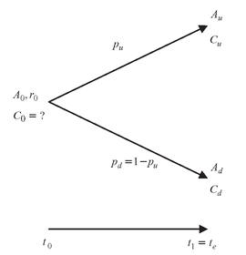
Our goal is to construct a portfolio today (t = t0) so that its value at expiration, te, replicates the value of the contingent claim. Therefore if we are the seller of the option, we can replicate the option′s contingent cash flows at expiration via this replicating portfolio. The fair price of the option today, C0, would be the cost of setting up the portfolio.
Our portfolio consists of taking a position in the asset, Δ units of it, by financing it via a risk-free loan of size L at the prevalent risk-free rate r until expiration date te, so the value of the loan at expiration would be L(1 + r × (te - t0)) = L/ D(t0, te ) regardless of the state of the world.
At expiry, te, if we are in Au state of the world, we want this portfolio to be worth Cu:
Δ × Au + L/ D(t0, te ) = Cu
Similarly, if we are in Ad state of the world, we want the portfolio to be worth Cd:
Δ × Ad + L/D(t0, te ) = Cd
We have two equations and two unknowns (Δ, L). Solving for these, we get:

Therefore, today′s value of the contingent claim is:

The seller of the option can charge C0 as above, make a loan of size L as above, and use these proceeds to buy Δ units of the asset at spot price A0. At expiration, in either state of the world, Au or Ad, the value of his holdings (Δ units of the asset) exactly offsets his liabilities: repayment of loan plus interest, and cash-settlement value of the option (Cu or Cd).
Note that in the preceding setup, we did not have to consider the probability of either state happening! As long as Au, Ad can happen and are the only two possibilities, we are golden!
A bit of algebra allows us to rewrite the formula for C0 as follows:
where
C0 = D(t0, te ) [ puCu + (1—pu)Cd]
No Arbitrage
Lack of arbitrage is equivalent to pu being a probability,
0 ≤ pu ≤ 1
Consider the case pu > 1, which means that A(0)/D(t0, te) > Au > Ad. We can sell the asset short today, and lend the proceeds, A0, until expiration. At expiration, we receive A0/D(t0, te), and need to pay either Au or Ad to cover our short. Regardless, we have made money with no risk!
Similarly, if pu < 0, then A0/D(t0, te ) < Ad < Au. In this case, we take a loan of A0 to buy the asset today. At expiration, we owe A0/ D(t0, te) while we own an asset that is worth Ad or Au. Regardless, we can sell the asset and pay off the loan for positive profit and no risk! Therefore, if there is no arbitrage in the above simple economy, pu can be considered as a probability, and today′s value of the option is simply the expected discounted value of the option payoff under this probability.
Risk-Neutrality
We obtained C0 by constructing a portfolio that replicates the option payoff, regardless of the probability of each state. We then showed that we can get the same value by taking the expected value under a probability pu. Other than a mathematical identity—pu is the probability that gets you the correct option value, as long as you know the option value!—is there another way of interpreting pu? The answer is in the affirmative: pu is the probability that a risk-neutral investor would apply to the above setting.
Most people are risk-averse: between a guaranteed return and a risky investment with identical expected returns, they would opt for the former. That is why risky investments (stocks, real-estate, . . . ) need to have higher-than-average expected returns. Otherwise, one could simply put one′s money in the bank and have the same return with no volatility.
On the other hand, most of us have bought a lottery ticket or played in casinos, investments whose expected gain is less than what we paid for. These types of investing are examples of risk-taking, where although risky, we are batting for the fences.
In between, there is an investment behavior that considers any investments with the same expected return as equivalent, and does not require a risk premium for risky bets. Consider such an investor given a choice between two investments: (1) invest A0 at the bank, and get A0/D(t0, te) at te, or (2) buy an asset at A0 and either get Au or Ad at te. For a risk-neutral investor, these two investments would be equivalent if
or equivalently, when
pu Au + (1 - pu) Ad = A0 / D(t0 , te)

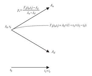
FIGURE 5.2 No-Arbitrage Requirement
Therefore, rather than setting up a replicating portfolio and computing its value today, we can simply take the expected discounted value of the option payoff using risk-neutral probabilities.
Relationship to Forwards
Recall that for an asset with no interim cash flows, its forward price on t0 for te-delivery, FA(t0, te), equals A(t0)/D(t0, te). Therefore, a geometric way to interpret lack of arbitrage is that future states must bracket forward prices, that is, lack of arbitrage is equivalent to
(see Figure 5.2).
Ad ≤ F A(t0, te) ≤ Au)
Similarly, we observe that in our simple risk-neutral world, one-step expected future prices must equal forward prices:
Et0 [A(te )] = F A(t0 , te )
FROM ONE TIME-STEP TO TWO
The two-state setup is obviously too simplistic. Assets can take a variety of values at expiration. However, using the previous setup as a building block, we can arrive at more complex cases. The trick is to subdivide the time from now till expiration into multiple intervals, and for each state in each interval, generate two new arbitrage-free future states. With enough subdivisions, we can arrive at a richer and more real-life terminal distribution for the asset.
FIGURE 5.3 A Two-Step Binomial Model
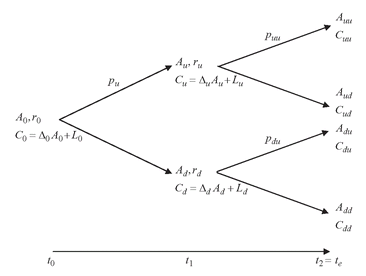
Consider the two-step model shown in Figure 5.3. If we have moved to the up state (Au, ru) by time t1, we have: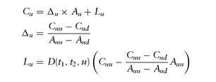 where D(t1, t2, u) is derived from the financing rate ru of the asset in the up-state for [t1, t2]:


We can get the same value via risk-neutral probabilities:

Similar equations hold if we have moved to the down state (Ad, rd) by time t1: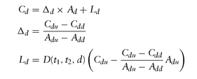 or expressed via risk-neutral probabilities:
 where
where


Having obtained Cu, Cd at time t1, we are back in familiar territory, and can solve for C0: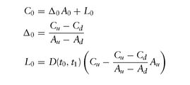 or equivalently,
 where
where


Rewriting the above equations, we have that risk-neutral probabilities must satisfy: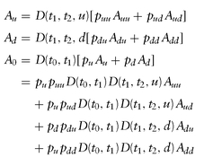

The above equations are written in short hand as: where ω denotes the generic random future path (uu, ud, du, dd).

Once we have computed risk-neutral probabilities satisfying the preceding, today′s and future′s price of any contingent claim is

Notice the similarity in the form of these equations for the underlying asset and contingent claims. As the asset itself can be considered as a trivial contingent claim—a claim whose payoff equals the underlying asset, C(t, ω) = A(t, ω)—the equations for the contingent claim are all we need to both characterize risk-neutral probabilities, and to value all contingent claims.
Path Discounting
Note that the preceding terms D(t1, t2, ω) are state-dependent, and reflect the short-term financing rates (expressed as discount factors) in each state:

This means that each final payoff C(t2, ω) has to get discounted back to today along the path of short-term financing rates (or discount factors) that lead to that final state. This is referred to as stochastic discounting or path discounting. We arrive at the core idea of risk-neutral valuation: The value of any contingent claim at any time, state, (t, ω), is the risk-neutral expectation of its stochastically discounted future cash flows.
Self-Financing, Dynamic Hedging
As we subdivide the time to expiration into finer partitions, we have to ensure that the original portfolio can be dynamically managed to replicate the option value. At each state, we can change the amount of asset we hold by securing requisite funds at the prevailing financing rates. As we do this dynamic rebalancing (changing Δs), we have to ensure that the value of the portfolio entering into each state equals the value of the portfolio leaving the state, that is, the replicating portfolio should be self-financing.
Consider the up state ( Au, ru). As we enter it, we hold a portfolio that consists of Δ0 units of the asset (now worth Au at t1), and a loan of size L0 plus its interest (worth L0/D(t0, t1) at time t1). Therefore the value of the portfolio value is:
Cu = Δ0 Au + L0 / D(t0 , t1 )
On the other hand, Cu = Δu Au + Lu, since (Δu, Lu ) is the required portfolio to replicate the option payoffs (Cuu, Cud) at the next time step t2. Therefore, we need to change our holding of the asset from Δ0 to Δu only by changing the size of our loan from L0/D(t0, t1) to Lu, that is, the change in the underlying holding should only be financed by the loan:
ensuring that the portfolio is self-financing.
(Δu - Δ0) Au = Lu - L0/ D(t0, t1)
Example in Two-Period Setting
To make the previous ideas clear, we consider a 2-month call option on $100M 2-year 5% semi-annual bond struck at par (K = 100%), where the time to expiration has been broken into two 1-month periods, Figure 5.4.
The seller of the option can replicate the option cash flows as follows:
( A0, r0) - Receive the option premium $0.945M today, borrow (in repo) $53.527M at 1-month repo rate of 4%, and use the proceeds, $54.472M (= $0.945M + $53.527M), to buy $54.472M face of the bond trading at full price of 100%. In 1 month, he will owe (repo) financing of $53.705M (= $53.527M × (1 + 0.04/12)), and will own $54.472M face of the bond.
FIGURE 5.4 Example of Option Pricing in a Two-Period Setting
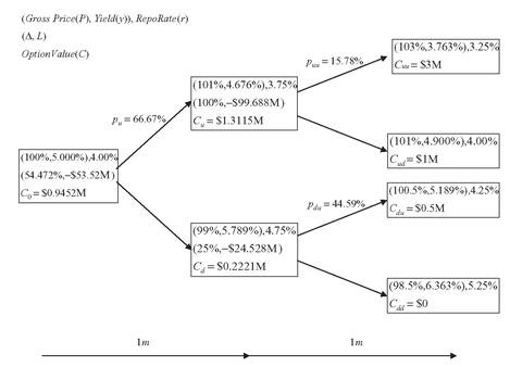
(Au, ru) - If we end up in the ( 101 %, 3.75 % )-state, the incoming value of our replicating portfolio is $1.312M = $54.472M × 101% - $54.472M. To replicate the option payoffs for the next period, we need to adjust our holding of the bond and the (repo) loan to (Δu, Lu) = (100%, -$99.688M), that is, we buy an additional $45.528M face of the bond at full price of 101% and finance $99.688M at 1-month repo rate of 3.75% to owe $100M = $99.688M × (1 + 3.75%/12) while owning $100M face of the bond in 1 month. In either future state, ( Auu, Aud), the value of our bond ($103M, $101M), minus the financing cost $100M, is exactly what we owe the option buyer: $3M, or $1M. Notice that while we rebalanced the portfolio, the outgoing value $1.312M (= $100M × 101% - $99.688M) is the same as incoming value, that is, the portfolio is self-financing.
(Ad, rd) - If instead, we end up in the (99%, 4.75%)-state, we need to reduce our bond position to Δd = $25M face, and change the repo borrowing to Ld = -$24.528M. Regardless of what happens 1 month later, the option seller will owe the (repo) financing of $24.625M (= $24.528M × (1 + 0.0475/12)), and own $25M face of the bond. If we end up in Adu = 100.5%, the option will be exercised for cash value of $0.5M, while we can sell the bond for $25.125M (= $25M × 100.5%), and pay $24.625M for financing, a wash. If instead, we end up in Add = 98.5% state, the option will not get exercised. The seller liquidates his $25M face of bond trading at 98.5% for $24.625M (= $25M × 98.5%), and uses these proceeds to settle exactly the financing cost ($24.625M). Again note that the incoming value, $0.222M (= $54.472M × 99% - $54.472M) is the same as outgoing portfolio value $0.222M (= $25M × 99% - $24.528M).
FROM TWO TIME-STEPS TO...
We can continue to subdivide the interval [t0, te ] into smaller short intervals. Let be partition of [t0 , te ] into N intervals, with 0 = t0 < t1 < · · · < tN = te , and let ri (ω) denote the financing rate at ti for [ti , ti +1], along ω, the random future state/path of the world. Then sitting at today t = 0, we only know r0, and if interest rates are nondeterministic, r1(ω), r2(ω), . . . , r N-1(ω) are all random. The generalized version of risk-neutral formula becomes
 where
where


Hence, each random payoff at expiration, C(tN, ω), has to get discounted along the series of random short-term financing rates that lead to that state of the world. Once we collect all these random payoffs and their corresponding random PVs, we can average over all possible states ω to arrive at today′s value.
RELATIVE PRICES
Focusing on the term multiplying the final payoff, we observe that the term
can be interpreted as the stochastic discount factor over the interval [t0, tN], while its inverse, M(t0, tN, ω), is the stochastic future value:
D(t0, t1, ω) × · · · D(tN-1, tN, ω)

As M(t0, tN, ω) is simply the value of unit currency reinvested at successive short term rates ri (ω), it is usually called the money-market account. Since M(t0, t0, ω) = 1, the risk-neutral formula can be rewritten as:

Expressed this way, we observe that the risk-neutral formula is just a simple condition on relative prices, that is, the value of any contingent claim relative to the money-market account, C(t, ω)/M(t0, t, ω).
No Expected Change in Relative Prices
In terms of relative prices, a characterization of risk-neutral probabilities is that at any point of time t0, the expected future relative prices, Et0 [C(tN)/M(t0 , tN)], are the same as the current relative prices, C(t0 )/ M(t0, t0). Relative prices have no expected profit/loss in a risk-neutral world.
This characterization evokes fair games from probability theory. For example, if we continually toss a fair coin with payoff of ±1 if heads/tails, then at any point, our expected future stake is whatever our current stake is, since the expected gain from each coin toss is 0. In probability theory, this is called the martingale property. In general, martingales are an abstraction of fair games, that is, processes that have zero expected change. In this language, relative prices are martingales under risk-neutral probabilities.
RISK-NEUTRAL VALUATION: ALL RELATIVE PRICES MUST BE MARTINGALES
We now have all the concepts for risk-neutral valuation. While the above discussion has been focused on a single risky asset, the arguments can be generalized to multiple risky assets, as established in papers by Harrison et al., and we refer the interested reader to them. We will be content with the following variant of their results: In a risk-neutral setting with multiple risky assets, all relative prices relative to the money-market account must be martingales. The all in the previous statement includes both the underlyings and contingent claims on them.
Focusing on the underlying tradeable assets in fixed income, that is, zero-coupon bonds, and their prices expressed as discount factors, since a te -expiry zero-coupon bond has unit value at te , the risk-neutral probabilities must satisfy

With this setup, risk-neutral valuation reduces to ensuring that the above is satisfied for all te ≥ t0 ≥ 0, and valuing contingent claims via:

Continuous-Time
By letting the number of time intervals N go to infinity, we arrive at the continuous-time version of risk-neutral formula. We let M(t, ω) denote the money-market account: started today (t = 0) with unit currency: M(0) = 1, where r (u, ω) denotes the instantaneous financing rate over [u, u + du] along the future random path ω. The martingale condition becomes
 for all futures dates t and maturities T, including any particular expiry T = te. This can also be expressed as

The above applies to all contingent claims. In particular, since discount factors at any time t are prices of unit currency at future dates T ≥ t, we have and today′s (t = 0) discount factors must satisfy
INTEREST-RATE OPTIONS ARE INHERENTLY DIFFICULT TO VALUE
Notice that as we were laying out scenarios for the future states of the world, for each state we had to specify both the underlying tradeable asset value and the short-term financing rates in that same state, that is, we had to consider the co-evolution of financing rates and the underlying tradeable asset. For example, for the 2-month bond call option, at each state we had to consider the bond price/yield and the repo rate. If instead we were looking to price an option on a swap, we would have to consider the underlying (forward) swap value and the financing (Libor) rate. As the value of a swap depends on the discount factor curve at each state, we would have to consider the evolution of the whole discount factor curve, a multidimensional problem. Of course, we can collapse all the information from the discount curve to the relevant underlying instrument (swap rate, swap value, bond price/yield), but still we would have to co-evolve this information with the financing rates.
This is in sharp contrast to pricing options on single stocks, FX, commodities, where the underlying is a single asset (1-dimensional), and since most of the risk is in the underlying, interest rates are conveniently assumed to be deterministic. For deterministic (nonrandom) interest rates, the stochastic discount factor can be replaced by its nonstochastic counterpart:
In this case, the discount factor can be taken outside the expectation, simplifying risk-neutral formula to:

For deterministic interest rates, contingent claim valuation then reduces to computing discounted expected payoffs, an easier feat than calculating expected discounted payoffs, which would require co-evolution of assets and interest rates. As we will in later chapters, by assuming certain terminal distributions (Normal, Log-Normal) for the underlying asset, we can get closed-form formulae (Black) for simple European options such as calls, puts, digitals. Due to their relatively simple structure and ease of quoting—much like flat yield-to-maturity for quoting bonds—these Black formulae and their variants are commonly used even for interest-rate options, despite the inconsistency of simultaneously assuming deterministic discounting and nondeterministic interest rates at expiration.
FROM BINOMIAL MODEL TO EQUIVALENT MARTINGALE MEASURES
We stated, ″In an arbitrage-free market, there exists an equivalent measure where assets′ prices relative to some numeraire are martingales. If the market is complete, this martingale measure is unique, and option prices are expected relative (to the numeraire) prices.″
Let us try to see if we can now parse the above and see their primordial counterparts in our simple CRR binomial model:
″Arbitrage-Free″: We showed that lack of arbitrage is equivalent to pu being a probability, 0 ≤ pu ≤ 1.
″Equivalent″: The asset possibility-space Au, Ad was fixed. We ignored the real probabilities, and focused on new (risk-neutral) probabilities. Note that we can only do this as long as we are interested in pricing contingent claims. The risk-neutral probabilities are not true-world probabilities, and should not be used to forecast future expected outcomes (although many people do!).
″Complete″: The assumption that option payoffs can be replicated via underlyings.
″Unique″: We set up two equations and two unknowns, and we could solve for Δ, L. If we had more unknowns than equations, the solution would be indeterminate, and hence not unique.
″Numeraire″: The currency relative to which asset prices are expressed. We selected the rolled-over money-market account, M(0, t, ω), as our choice of numeraire.
″Relative prices are martingales″: Et [C(T, ω)/M(T, ω)] = C(t)/M(t). This compact formula completely characterizes the risk-neutral probabilities, relating them to the assumed underlying asset value evolution, and also is the pricing operator for contingent claims.
Indeed, the two-step binomial model captures all the key ingredients of option pricing, and is all one really needs to understand the concept of risk-neutral valuation.
A final note is that the money-market account choice of numeraire, although common, is not required, and any positive-valued process can serve as the numeraire. For interest rate options, we chose the money-market account as this is the most common and intuitive numeraire. Chapter 11 picks up the discussion on the choice of other numeraires.
..................Content has been hidden....................
You can't read the all page of ebook, please click here login for view all page.
