Most modern web applications perform a relatively small number of writes but a large number of reads. This chapter will look into the most common activity your application will perform and how RavenDB supports it. We will learn the basics of Raven Query Language and the basics of querying using it.
Querying in RavenDB Studio
A screenshot of the documents page of the Raven D B studio. A list of collections and tabs labelled patch and query are on the left, and a number of documents are listed on the right.
Query Option Below List of Collections
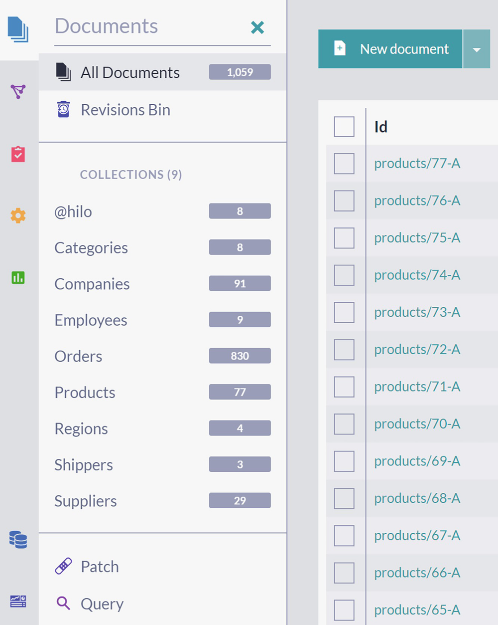
A screenshot of the query page has 2 panels. The top panel depicts a text box to enter the query. The bottom panel depicts space to display the results. To the right of the top panel is a play button, and 3 more buttons at the top.
Query Panel in RavenDB Studio
As you can see, this panel has two fields – the upper one where you write your queries and the lower one where the result of the query execution is displayed.
After you write a query, you can run it by pressing ctrl+enter on your keyboard or clicking on the Play button to the right.
The following section will look into the basics of querying with Raven Query Language.
RavenDB Query Language Basics
Raven Query Language or RQL is a SQL-like query language of RavenDB. Chapter 1 mentioned that relational databases share a standardized query language called Structured Query Language - SQL. This common declarative language was one of the significant success factors for RDBMS.
Compared to that, NoSQL databases do not have standardized query language. Considering the dynamic and decentralized nature of the NoSQL ecosystem, there is a low chance any standard will ever emerge. Hence, every time a new NoSQL database is incepted, authors have the tedious task of coming up with a query language for their database. And this assignment brings a heavy burden – once you decide and create language, developers will start using it to build applications. From that point onward, changes you can make to your query language are limited – any significant design change will break backward compatibility and annoy your users.
The team behind RavenDB faced the very same challenge. In the end, a decision was made to use SQL as a basis but to make several extensions and modifications that would make RQL a powerful language. That way, developers familiar with relational databases and SQL would recognize similar concepts and learn the basics of RQL quickly. Let us not forget – querying is the main activity we perform in applications, and fast queries directly contribute to the perception of your application speed.
Keyword “from”

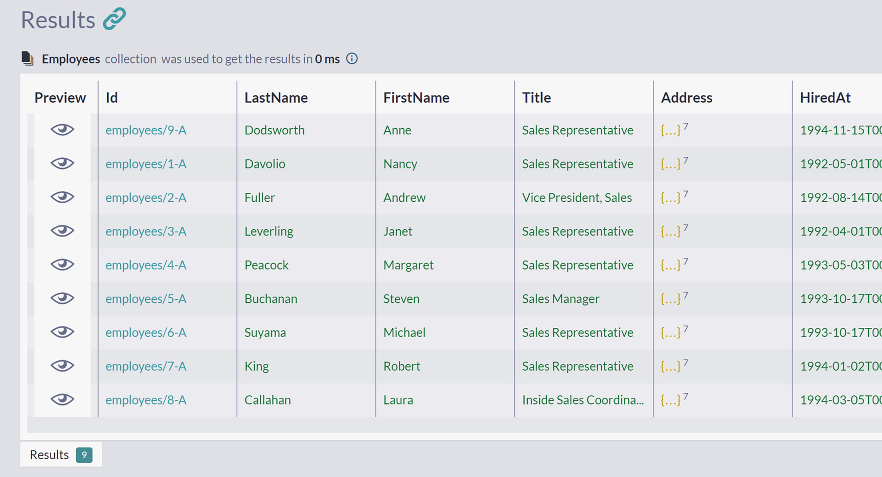
A screenshot of the query page has 2 panels. The text typed on the top panel reads from employees. The results panel at the bottom depicts 9 documents under the label employees, which are listed under 11 columns.
Selecting All Documents from Employees Collection

A screenshot of the result panel has 5 options at the top that are, delete documents, statistics, export as C S V, display, and expand result, in which display is selected. The selected options in the display are I d, last name, first name, title, address, and hired at.
Adjusting Visibility of Employee Properties
The initial configuration of visible properties will show you only some of them. If you would like to preview the whole document, there is a Preview icon in the first column of the table. Click on it, and you will get a complete JSON preview for a specific document.
Filtering
In the previous section, we learned from, first, and essential RQL keyword. It will be a part of every RQL query you make. We saw it used with a collection name, from Employees, to return all nine Employee documents.
Keyword “where”
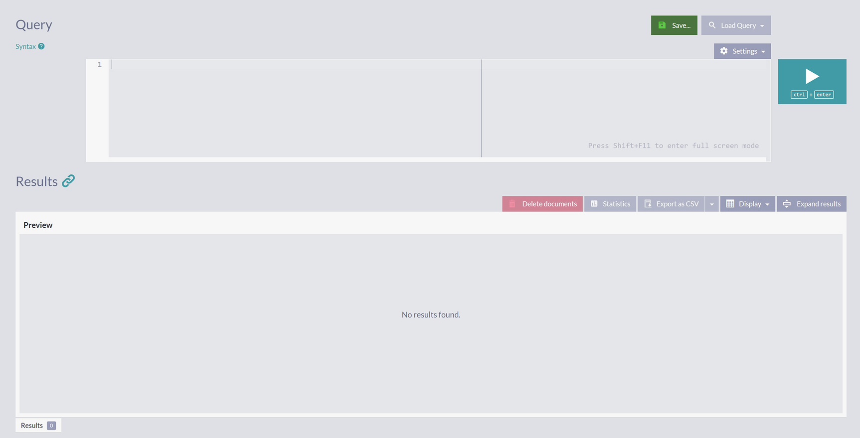
A screenshot of the query page has 2 panels. The text in the top query panel reads, from employees where last name equals fuller. The results panel at the bottom depicts a document in which the last name is fuller.
Filtering Employees by the Value of LastName Property
Filtering all Employees with the first name Andrew
Executing this query will produce the same result of just one document – Andrew Fuller has a unique first and last name on the company level .
which will produce the same result.
Query by Nonexistent Property
Filtering all Employees by absent property
In Listing 3-4, we made an intentional typo – FistName. If you are a developer accustomed to relational databases, you will expect to receive an error upon executing this query.
However, in RavenDB, an attempt to filter a collection by the nonexistent property name will not produce any errors. You will get an empty result set. Why is that? If you recall, RavenDB is a schemaless database. In relational databases, a schema is a set of mandatory fields for each table. The schemaless nature of RavenDB collections means the absence of any compulsory structure imposed upon documents belonging to the same collection. There is no such thing as a set of mandatory properties such documents must have. Hence, filtering by any property name you can think of will not produce an error – it may only make an unexpected empty result set.
Query by Non-string Properties
Filtering by Complex Properties
Structure of Employee JSON Document
Filtering all Employees by nested property
Query from Listing 3-6 will select all employees living in the United States. Pay attention to the format of the property name Address.Country – looking at the JSON from Listing 3-5, you will observe that Country is a nested property within Address property.
Transforming the nested structure of JSON properties into a linear form suitable for filtering queries is straightforward. You will write parent property on the first level (in this case, Address), and then add desired property from the second level (in this case, Country), separated by a dot.
The same approach is applied with properties on deeper levels. Hence, to filter by Latitiude property visible in Listing 3-5, we will first state top-level ancestor Address and then descend over Location to the Latitude. Every time we go one level deeper, we will add a dot as a separator between property names. Hence, our final flattened form is Address.Location.Latitude. When reading this concatenated property from left to right, you descend one level every time you run into a dot.
and will return all employees living along specified Latitude.
Filtering by Id
will return an empty result set, even though we can inspect that employee with id employees/2-A exists.
Why is this the case? As we saw in the previous chapter, an identifier is a unique property called @id located within @metadata. However, this is a default location of an identifier which is also configurable. Because of this, you need to use function id() that will return the name of the property holding the document identifier .
and results will show this is our old friend, Andrew Fuller.
Cross-Collection Query
will find all documents across all collections with a FirstName property containing value Andrew. This query result is the same as Listing 3-3, where we specified the collection name. The reason for this is apparent – only Employee documents have FirstName property.
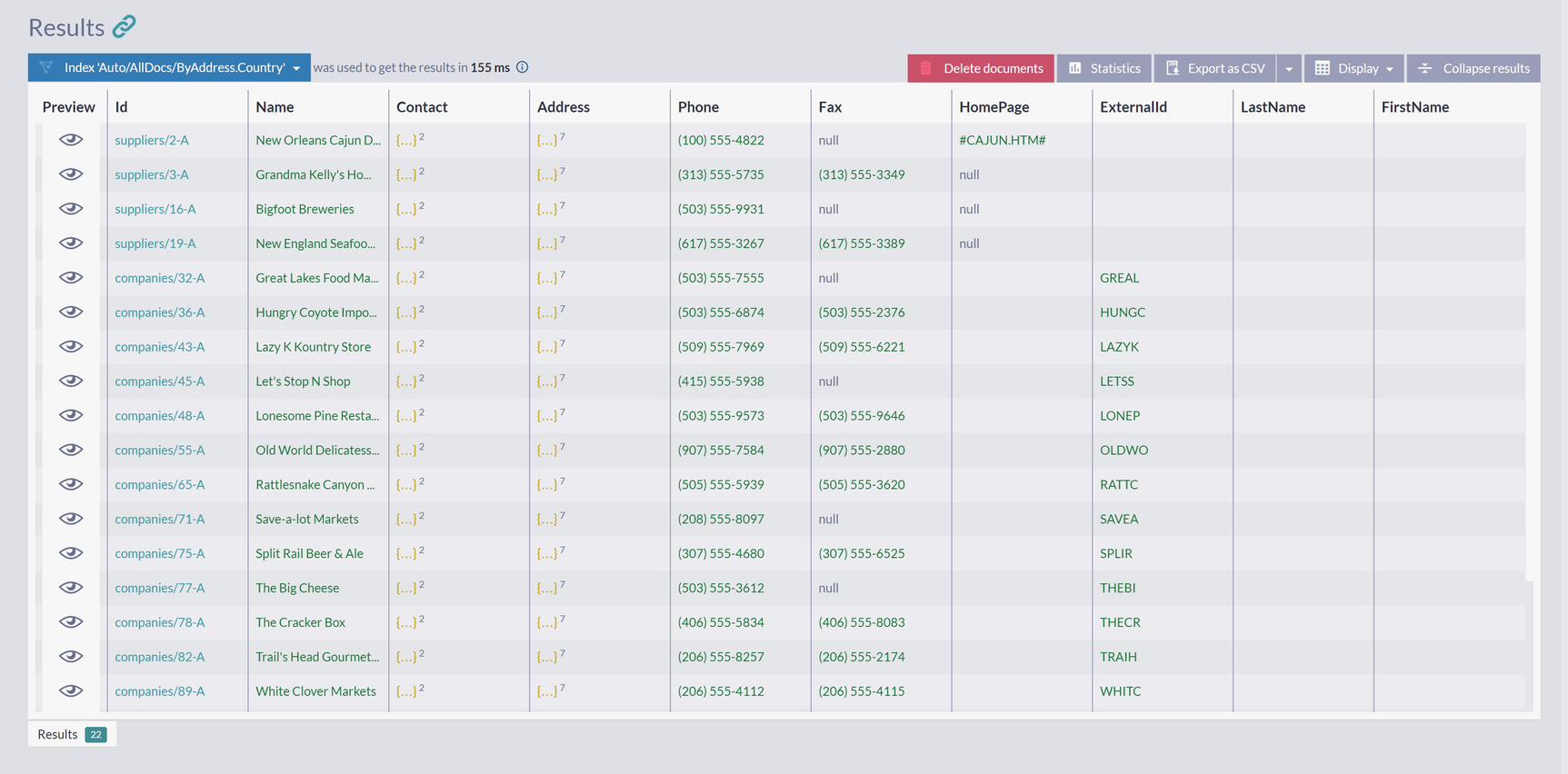
A screenshot of the results panel on the query page has a list of documents under the label, index auto slash all docs slash by address country. The documents are listed under the column labels: preview, I d, name, contact, address, phone, fax, home page, external I d, last name, and first name.
Result of a Query Across All Collections
This query returned 22 documents in total from Suppliers, Companies, and Employees collection. All these documents represent business entities located in the United States.
will return a total of 129 documents that contain Country property within Address property. However, pay attention that this will also return those documents containing a null value for a specific property. From the perspective of RavenDB, nothing is distinguishing null – it is a regular value property can have. Hence, exists() will check the presence of a specified property, ignoring its content .
Inequality Query
will select all Employees where the first name is not Andrew.
Logical Operators
IN operator accepts a list of values and will return true if the stated property has any of the values from the list.
This query will return two products, products/34-A and products/67-A, which have 16 units in stock and cost 14 per unit.
and shorten it. However, a query like this will always return an empty result set – you cannot have a property with two values at once. And, indeed, the single value of a simple property cannot, but complex property that contains multiple values can.
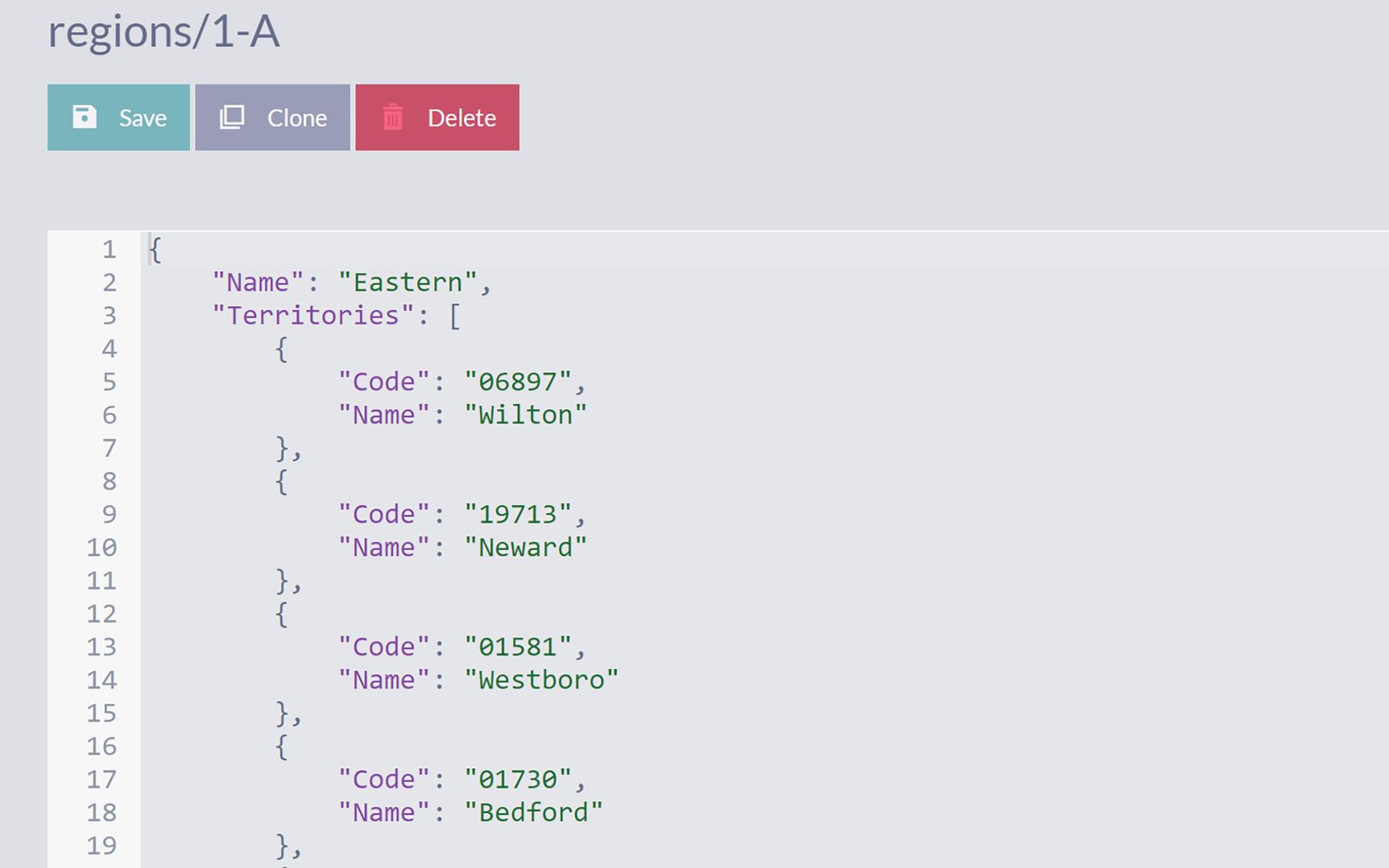
A screenshot depicts a document titled regions slash 1 A. The options below the title are, save, clone, and delete. The document depicts 19 lines of code.
Region Document
We can observe two interesting features here. The first one is ALL IN operator that provides a way to match multiple values against an array. The second one is the expression Territories[].Name which is taking all elements of Territories collection and extracting Name property from every element.
A typical use case of the ALL IN operator is selecting all documents tagged with a specified set of tags .
Range Queries
So far, we have been using equality and inequality operator to filter by exact matches. It is also possible to use additional operators to create range queries .
will list all products with 26 or more units in stock. We will leave as an exercise usage of analogous operators < and <=.
lists all products that have one, two, or three units in stock.
Note that BETWEEN is inclusive on the lower and higher end of an interval .
Casing
Even though you might expect no results, since we capitalized all letters in the name, this query will return Andrew Fuller as the only result. Why is that?
RavenDB defaults to case-insensitive matching in queries. In this case, the value of the filtering condition was different from the actual property in the document, but Andrew and ANDREW matched since RavenDB ignores casing differences. This case insensitivity was a conscious decision since, in most scenarios, case-insensitive comparison of strings will produce results as you desire.
Full-Text Searching
The ability to perform a full-text search over data is one of the standard features in modern applications. This kind of search will inevitably be present in most of the applications you will be building over time. Fortunately, this is one of the areas where RavenDB excels. We will provide more information in chapters to come, but for now, let’s just say that RavenDB uses Lucene.net internally for indexing purposes. Lucene is one of the best indexing engines available today, and over the years, it has established itself as a reliable and standard solution. As a part of an infrastructure, it has been present in several brand-name products, like Solr and Elastic Search. So, RavenDB can provide you with first-class full-text searching capabilities and eliminate a need for any additional solution that would provide you with this.
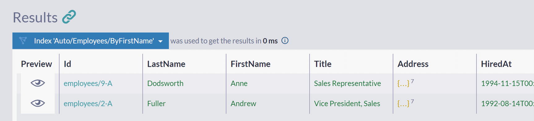
A screenshot of the results panel in the query window has 2 documents under the label, index auto slash employees slash by first name. The first names in the 2 documents are Anne and Andrew, respectively.
Searching Employees by the Prefix of FirstName
We got two results, two employees, both having first names that start with “an.” Note that in this case, we have a case-insensitive query as well.
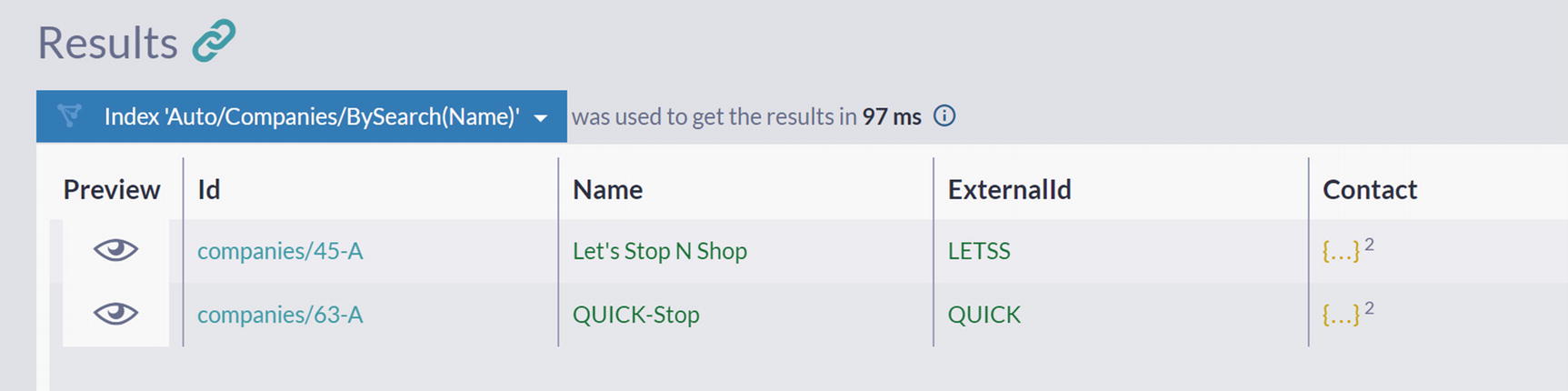
A screenshot of the results panel in the query window has 2 documents under the label, index auto slash companies slash by search name. The names in the 2 documents are let’s stop N shop and quick stop respectively.
Searching Companies by the Name Content
Both of these companies contain the word “stop” as a part of their name .
It is clear what happens when we perform equality filtering, where exact matching is done, but what happens behind the scene in this case, where partial matching on the arbitrary position can happen? To provide this functionality, RavenDB will take the Name of the company and apply tokenization: the name will be split into words, and every such word will be indexed. As an example, the company name “Let’s Stop N Shop” would be divided into four tokens: “Let”, “Stop”, “N”, “Shop”. After you execute a full-text search query, RavenDB will match your search term against a set of tokens and show you results. So, you could say that full-text search is still exact matching, but not against full property value – instead, components (tokens) are matched.
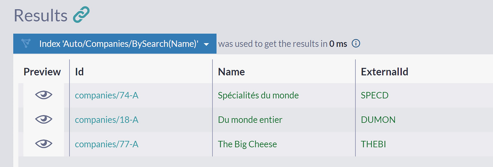
A screenshot of the results panel in the query window depicts 3 documents under the label, index auto slash companies slash by search name. The names in the 3 documents are spécialités du monde, Du monde entire, and the big cheese respectively.
Searching Companies by the Name Content with Multiple Terms
you will get a list of companies located in London or Sweden. As you can see, all properties of the Address are indexed, so the full-text search is simultaneously checking both City and Country fields .
Sorting
A screenshot of the results panel in the query window has 9 documents under the label, employees. The documents are listed under the column labels: preview, I d, last name, first name, title, address, and hired at.
Unsorted Listing of All Employees
will apply secondary sorting by the first name in all those cases when two employees have the same last name.

A screenshot of the results panel in the query window has a list of documents. The documents are listed under the column labels: preview, I d, name, supplier, category, quantity per unit, and price per unit.
Sorted Listing of All Products
However, looking closely at the column PricePerUnit reveals it is not sorted in the descending order as we expect. Why is this happening , and how to correctly sort Products by this column?
The cause of this lies in the way that RavenDB treats stored data. Fields are not typed, and without us expressing intention, RavenDB will default to lexical ordering, i.e., fields are treated as strings by default. With descending lexical ordering, 81 will come before 9, and that explains the sorting order we got.
Paging
will filter companies from the United States, order them by name in ascending order, skip the first five, and take the next five .
Advanced Querying
In the previous section, we saw an introduction to RQL and basic filtering, ordering, and paging operations. Now we will look into advanced functions – projections, aggregations, and includes.
Projecting Results
Usage of select keyword
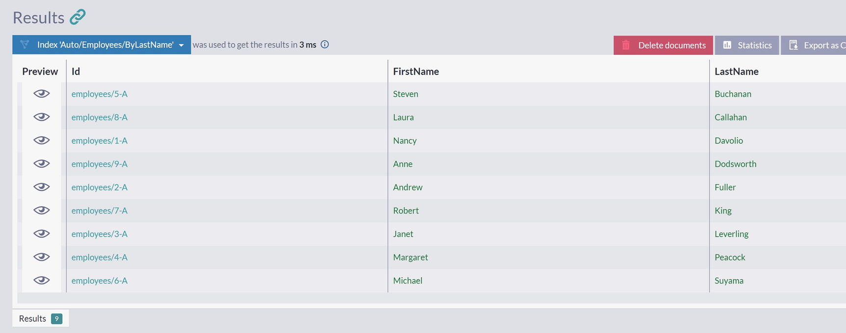
A screenshot of the results panel in the query window has 9 documents under the label, index auto slash employees slash by last name. The last names in the list of documents are in ascending order.
Results of Using Select Keyword
As you can see , select is very similar to the SQL variant – it will select and return only a subset of fields.
ShipTo object is selected as it is, and Products property contains projection composed of product name selected from all order lines.
Projecting with Object Literals
Projecting with object literal
As you can see, we used a simple path to select shipping country and complex expressions to perform a deep selection of first and last product from order lines collection. Notice that in Listing 3-8, we had to use an alias as o to be able to reference o in complex projection expressions.
Projecting with JavaScript within object literal
Id – calling function id() that is taking document as an argument and determines its identifier.
Year – calling JS constructor for Date object with ISO 8601 string as an argument. After that, method Date.getFullYear() returns year.
Fullname – concatenates two properties of the document with a separator.
Declaring Functions in Queries
Calling JavaScript function from object literal
In this example, we extracted code that was joining first and last name into function getFullname() , which is then called from object literal .
Example of complex JavaScript code in object literal
Aggregation
Aggregation is the process of grouping data. In this section, we will examine how RQL can provide data aggregations and enable you to sum up your documents in various ways.
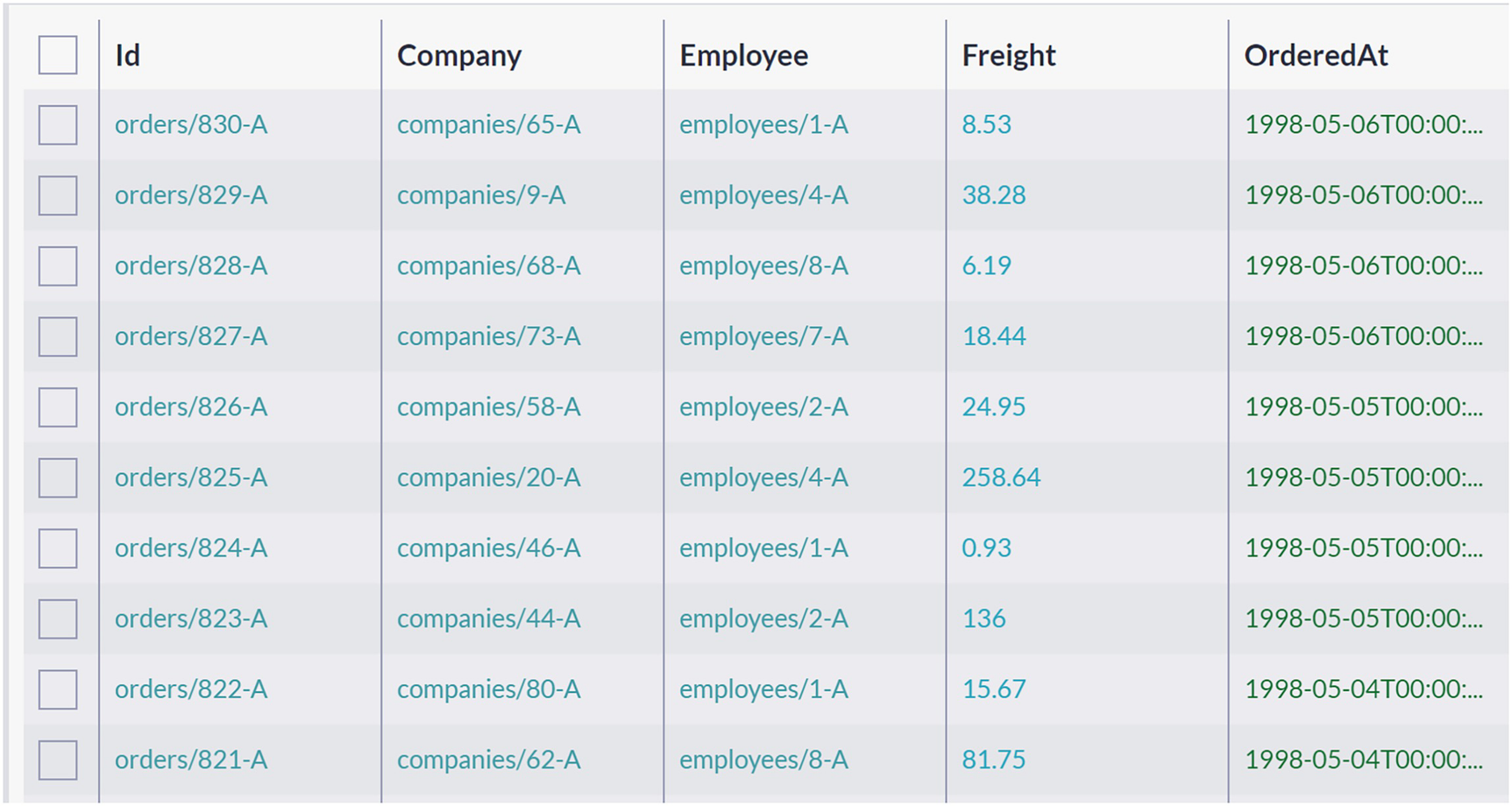
A screenshot of a table has 5 columns and 10 rows. The column labels are I d, company, employee, freight, and ordered at.
Orders have Company Property with Company Identifier
Grouping orders by companies

A screenshot of the results panel in the query window has 7 documents under the label, index auto slash orders slash by count reduced by company. The documents are listed under the column labels: preview, company, and count.
Orders Grouped by the Company
Compared with the previous query, you will notice a new line load Company as c. Load command will instruct RQL to load the document with id contained in property Company and assign it alias c. After this is done, we can access the company’s name in the last line by referencing c.Name. Finally, we can show our users that “Save-a-lot Markets,” “Ernst Handel,” and “QUICK-Stop” are 3 companies with more than 20 orders.
In most applications, aggregation queries are the primary tool for fetching helpful information from the database. RQL aggregating basics we just demonstrated are one way of summing up data. RavenDB has another much more powerful mechanism, which will be covered in chapters to come .
Handling Relationships
In the previous chapter on Modeling, we learned about suitable and appropriate modeling principles that will result in documents with a balanced level of independency, isolation, and coherency. However, even with such documents, you will still need to combine them into view models that combine properties from two or more documents into a form suitable for visual representation . Let’s look at how RavenDB can support you in such scenarios.
Accessing Related Documents
Displaying the order in this form to the user does not bring too much value – the user would have to check which company hides behind id companies/65-A manually.
Loading reference Company and Employee
As you can see in Listing 3-13, we provided load with a list of references and aliases for dereferenced documents. After that, in select projection, we can use documents c and e.
From
Where
Load
Select
RavenDB will take the from-where part of the query and run it, producing interim results. After that, RavenDB will execute load() to fetch documents referenced from interim results. Finally, select will create a projection that is the final result set of this query. It is essential to note the order here – load is applied in the end, after results have been filtered and fetched and basic query execution completes. Because of this, load() does not impact the cost of the query.
If you compare this with relational databases, you will see that the order of execution is significantly different. You would write a query that would first perform join that would provide access to referenced rows and then apply filtering on joined tables. However, please pay attention that we would join all rows from these tables and then perform filtering. In other words, the RDBMS engine would spend cycles joining rows, only to discard them after filtering is applied. RavenDB optimizes not only on this but also on many other things. As a result, your applications will be faster, and the amount of work for the same queries will be lower.
Include

A screenshot of the results panel in the query window has a document under the label, orders. The document is listed under the column labels: preview, I d, company, employee, freight, and lines.
Order with Included Company and Employee
At the bottom of Figure 3-16, you can see two more result sets. Since we have just one order returned, these two collections contain just one company and just one employee.
Include syntax is intended to be used when you want to fetch the complete document from the database and pull along all related documents in the same round trip to the database. You will then perform some additional operations on these documents without being forced to make any more requests to the database.
Summary
In this chapter, we covered writing queries in RavenDB. Besides filtering, querying, and paging, we also covered advanced topics - projections, aggregations, and dereferencing relations.
In the next chapter, we will introduce indexes, a crucial data structure all databases use to optimize and speed up queries.