We already mentioned the full-text search capabilities of RavenDB in Chapter 3, and this chapter will expand on the concepts introduced there. We will show basic search capabilities, including operators, wildcards, and ranking. You will learn what lies under the hood and how RavenDB indexes process text internally to provide all these capabilities. Finally, we will demonstrate how you can take more control over the indexing process and apply advanced techniques with static indexes.
Basics of Full-Text Search
Looking at standard features in modern applications, you will quickly realize that ability to perform a full-text search is high on this list. Almost every application needs it. With a large amount of data, the ability to search becomes crucial; information that is not readily retrievable is essentially unusable.
In previous chapters, we saw how to perform filtering based on the exact match – you would specify the property name and value, and the database would return one or more documents where a property has that value.
The beauty of full-text search is partial matching – you can search for a particular term that is part of a text. For example, you can locate all books with a title containing “London” or all products with “chocolate” in the name. You can also specify prefixes or suffixes and get all matching documents. It is possible to pass multiple terms, and the database will return a union of documents containing any of those terms.
Let’s look at various ways you can search text with RavenDB.
Single Term
A table of 11 product names and identification. The products I D are 77-A, 76-A,75-A, 74-A, 73-A, 72-A, 71-A, 70-A, 69-A, 68-A, and 67-A.
Names of Products
This query will return products with the names Tofu and Longlife Tofu. A term you search for can be at the beginning, the end, or anywhere inside the product name; RavenDB will easily match any position.
With default settings, the full-text search feature in RavenDB is case insensitive.
“tofu”
“ tofu “
“-tofu,”
Multiple Terms

A table of the results of the term tofu vegie. The labeled index are preview, identification, name, supplier, category, and quality per unit.
Search Results for the Terms “tofu vegie”
thus, including products containing any of these terms in the Name property .
Searching over Complex Objects
A nested structure of Address property of Employee document
In this case, RavenDB correctly processed complex nested structures by flattening them and indexing all properties from various levels.
Wildcards
Partial matching of full-text search provides a way to specify a word for searching within the text. Wildcards can increase the power of partial searching – you can replace one or more letters in situations where the beginning or end of a search term is unknown.
Executing this query will return Andrew and Anne.
This query will return Steven Buchanan and Laura Callahan from our sample dataset.
This infix full-text search will return Anne, Nancy, Andrew, and Janet.
When using wildcards, one more critical factor to consider is performance. Using a leading wildcard drastically slows down searching. Of course, this slowdown will not be significant on small datasets (like the current sample dataset we are using). Still, it may become a factor as the number of documents in your database increases. Hence, you should bear that in mind and evaluate every suffix full-text search scenario, both for justification and for potential negative impact .
Create a static index where you would index reversed text, thus transforming leading wildcard searches (search by suffix) into trailing wildcard searches (search by prefix).
Create a static index with a non-default analyzer.
Later in this chapter, we will cover the second technique .
Suggestions
Selecting suggestions

An algorithm depicts the results and searches the suggestion for the term 'chai', and 'chang'. The labeled indexes are preview and name.
Suggestions for the Word “chaig”
Suggest function will find words similar to the term passed, based on the calculated distance algorithm value. This is handy if you want to implement Google-style “Did you mean?” suggestions.
Operators
and will return all employees living either in Seattle or London.
will return no results since there is no Employee with both cites in the address.
This query will return employees who either are managers or speak both Spanish and Portuguese languages.
What Happens Inside?
Looking at various ways to perform partial searching demonstrated in the previous section may lead you to think many complex things are going on. And even though the full-text search is not a simple mechanism, most of the inner implementation concepts are relatively simple. As we already saw with filtering, ordering, and aggregations - it all comes down to using appropriate data structures. Next, to avoid computation during query time, which is always dangerous since the query’s execution time depends on the dataset’s size, RavenDb will prepare index entries upfront. As a result, full-text search is efficient and fast. A certain amount of work is imminent, but doing it at most once, ahead of time, and storing the outcome for reuse is the key to performant queries.
Text Analysis
During indexing , RavenDB will use an analyzer to separate text into segments. These segments are called tokens, and they will form index terms. Later, when you perform a full-text search, your search term is matched against tokens contained in an index. Hence, this approach will transform a partial match of a search term against text into an exact match against the collection of tokens produced during the analysis of the text. Of course, this statement simplifies the whole process but conceptually describes the matching mechanism well.
Primarily, the analyzer performs tokenization of the text. Tokenization breaks text into lexical units, also called tokens. Tokens are the shortest searchable units, and the tokenization process converts input text into a token stream.
Additionally , tokens produced by a tokenizer are passed through one or more filters. Filters will examine the token stream and may leave tokens intact, modify them, discard them, or even create new ones. Alterations may include normalizing characters to all lower case or a version without diacritics. Punctuation and stop words like the and is are often removed, as are other unhelpful tokens that might impact the search quality.
Tokenizers and filters are usually combined into a pipeline (also called chain sometimes) where the output of one is input for another. The analyzer is simply a term for a sequence of tokenizers and filters that take text as input and produce a set of tokens.
Standard Analyzer
RavenDB comes with several analyzers, with Standard Analyzer as a default one. Standard Analyzer consists of Standard Tokenizer and two filters – LowercaseToken Filter and StopToken Filter.
Standard Tokenizer will perform segmentation of text by treating whitespaces, newlines, interpunction, and other special characters as token boundaries. Such generated stream of tokens is passed through LowercaseToken Filter, which will normalize them to all small letters. Finally, StopToken Filter will remove English stop words from the token stream. Examples are a, the, and is – these are so-called function words , which are ambiguous or have little lexical meaning in the context of full-text search.
This process will remove exclamation marks and common words like a and the. Additionally, all tokens are lowercased.
As we have seen in previous chapters, running various queries will trigger RavenDB to create appropriate indexes to serve those queries efficiently. Likewise, RavenDB will create an automatic full-text search index when you run a full-text search query. Standard Analyzer will be applied to one or more searched fields. Their content will be tokenized, and a set of index entries will be generated.
RavenDB will apply Standard Analyzer to string “Andrew Anne” transforming it into a token stream [andrew], [anne] and only then perform actual matching of these tokens to indexing terms. This rule has one exception – if a search term contains a wildcard, it will remain. An analyzer is not applied to search terms containing wildcards .
Keyword Analyzer
LowerCase Whitespace Analyzer
NGram Analyzer
Simple Analyzer
Stop Analyzer
Whitespace Analyzer
You can use some of these to populate your full-text search index with differently shaped tokens. We will cover one such case later in this chapter.
Finally, RavenDB supports custom analyzers. Depending on the circumstances, you may have specific needs for tokenization and filtering. In such situations, you can write your custom analyzer and supply it to RavenDB. A typical example is the analysis of content in different languages. You can already guess that set of stop words is language-dependent. For example, the English word car is among the stop words in the French language. Custom analyzers are out of the scope of this book, but it is good to be aware of the highly customizable nature of RavenDB.
Ranking
For full-text search results to be helpful and for users of your application to be satisfied, most relevant results should be ranked at the top, followed by less relevant results. How does RavenDB determine relevancy?
Let’s look at some examples.
you will notice results are sorted in reverse order compared to the previous query, following the order of search terms – first employee from Redmond and then two from Seattle.
Searching for multiple terms
This query will rank London employees first and then Seattle employees, and finally, any Redmond employees will be at the bottom of the list.

An algorithm for the index score of document employee/4-A. The labeled query is address city, metadata, flags, identification, last-modified, change-vector, projection, and index-score.
The Indexing Score Located Within the Metadata

An algorithm for the ranking scores of employees. The labeled index are show, identification, and explanation. The I D are employees/4-A, employees/8-A, and employees/1-A.
Explanation Column with Ranking Scores

An algorithm depicts the detailed explanation of the index scoring for employees/4-A.
A Detailed Explanation of the Indexing Score
This decomposition can help you determine why specific results ordering is the way it is.
Boosting
Not all search terms are created equal. Sometimes, you would like to value specific search terms more than others. Boosting is a process of altering weight factors – so you will be able to make some search terms more relevant compared to others. As we saw in a previous section, RavenDB will assign a weight factor to each word and use it to calculate the index score for every matched document.
Each search term can also be associated with a boosting factor. The higher the boost factor, the more relevant the search term will be. This feature can improve the accuracy of the results, ordering documents so that more relevant ones are at the top of the result list.
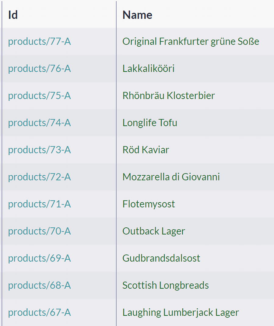
Full-text search query with boost() function applied
A table of results for the 9 companies. The labeled index is the preview, identification, and address/city. The companies and addresses are 57-A, 74-A as Paris, 4-A,11-A, 16-A,19-A, 53-A, and 72-A as London, and 89-A as Seattle.
Result Ordering Modified with boost() Function
Boosting query with included explanations

An algorithm depicts the explanation tab with computed scores for 9 companies. The labeled index are show, identification, and explanation.
Explanation Tab with Computed Scores
You can click on the Show icon for a further breakdown of how these scores were calculated .
One more possibility to leverage boosting is to make specific fields more relevant. For example, we might need to locate all employees with managerial capabilities. A good candidate for searching is Title and Notes field. However, these two fields are substantially different – while Title contains a current position with the company, Notes contains an employee’s description that may mention various skills and previous jobs. Employees in current managerial positions are more relevant than those with administrative functions in the past .
Boosting of Title over Notes

An algorithm depicts the results of the execution of employees. The labeled index are preview, identification, last name, first name, title, and notes.
Results of Boosting Title over Notes
As you can see, Steven is ranked higher than Andrew since he has the word Manager in the Title field. Using this approach, you can fine-tune ranking and provide better accuracy.
Static Index: One Field
Products/ByName index
Before saving the definition of this new index, there is one more step you need to take – specifying that Name is not an ordinary field but a full-text search field. You need to mark the index field Name as a field that will be treated as a full-text search field.

A table of field options. The labeled field is name, store, highlighting, spatial, advanced, term vector, analyzer, full-text search, suggestions, and indexing.
Field Options
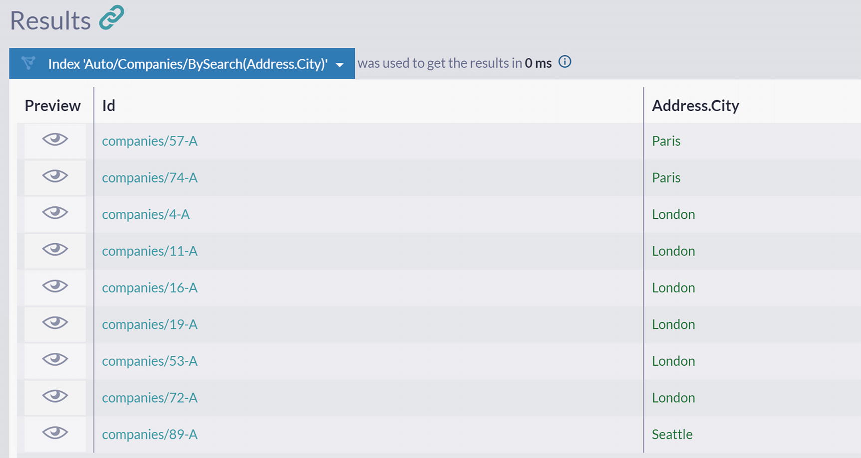
A table of the standard analyzer index terms for products and names. The index process 16 products.
Standard Analyzer Index Terms

An algorithm depicts raw index entries. The labeled entries are cache enabled, don't create a new auto-index, show stored index field only, show raw index entries instead of matching documents, and ignore the index query size limit.
Raw Index Entries
Static Index: Different Analyzers
In one of the previous sections, we mentioned that using wildcard prefixes can have a significant impact on performance. The static index gives us total flexibility, so we can configure the indexing process to overcome challenges like this.
One possible solution would be to alter the way index terms are calculated. We can change tokenization - instead of Standard Analyzer, we can use NGram Analyzer.
But what does the word NGram means? NGram is a sliding window that moves across the text and produces tokens of the specified length. For example, word “brown” can be split into the following 3-grams: [bro], [row], [own]. Similarly, applying 2-grams tokenization to “jumps” results in stream [ju], [um], [mp], [ps].
NGram tokenizer available in RavenDB will slide windows of sizes 2, 3, 4, 5, and 6 to produce tokens of various sizes. Along with this tokenizer, the NGram analyzer will use StopWords and Lowercase filters.
For example, for sentence
The quick brown fox jumped over the lazy dogs.
The StopWords filter will eliminate two occurrences of “the” and the full stop.
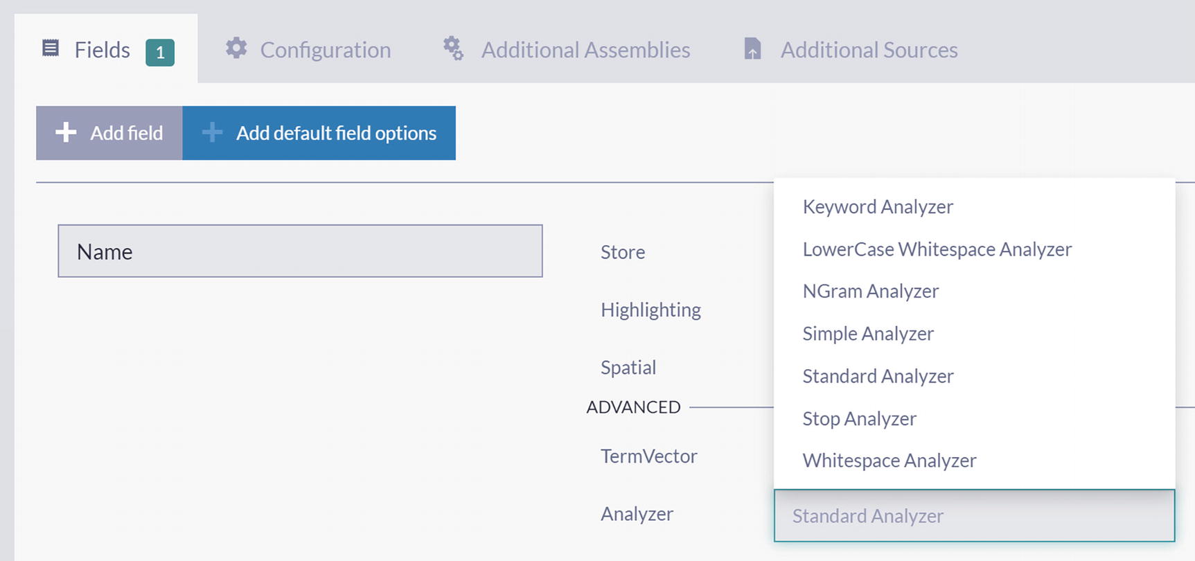
An index depicts changing index analyzer. The labeled analyzer are keyword, lowercase whitespace, N-gram, simple, standard, stop, and whitespace analyzer.
Changing Index Analyzer
After selecting NGram Analyzer, save redefined index.

A table of the N-gram index terms for the products and names. There are 16 labeled terms.
NGram Index Terms
These index terms are different compared with tokens generated by Standard Analyzer. Index terms produced by the NGram analyzer are the union of 2-grams, 3-grams, 4-grams, 5-grams, and 6-grams over product names.
which will return the same result set but without any performance penalties.
Static Index: Multiple Fields
We defined and configured an index covering just one field in the previous two sections. This section will show how you can expand it to process multiple fields from documents belonging to one or more collections.
Indexing Property from Multiple Collections
We can expand Products/ByName into an index that will provide a way to search not only products by name but also Suppliers and Companies by name. This way, we will create one index that will cover the content of the documents from three collections.
Start by cloning the Products/ByName index – click the Clone button and change the name to Search/ByName.
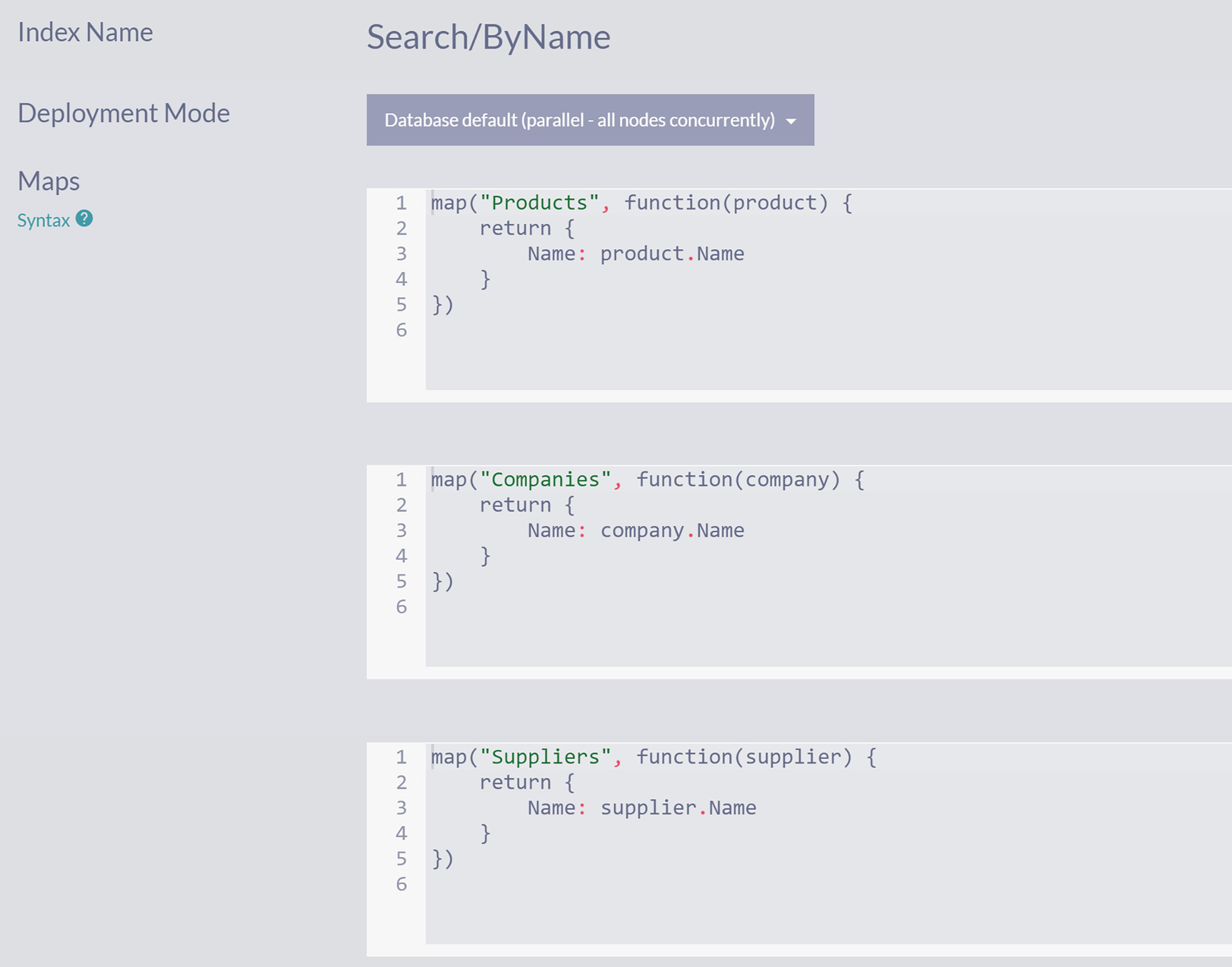
Three algorithms depict the index definition of the product, companies, and suppliers. The labeled fields are index name, search/by name, deployment mode, and maps.
Search/ByName Index
Since we started by cloning the existing index Products/ByName, your newly created index supports full-text indexing on the Name field out of the box.
Now you can execute search queries that will span content from three collections.
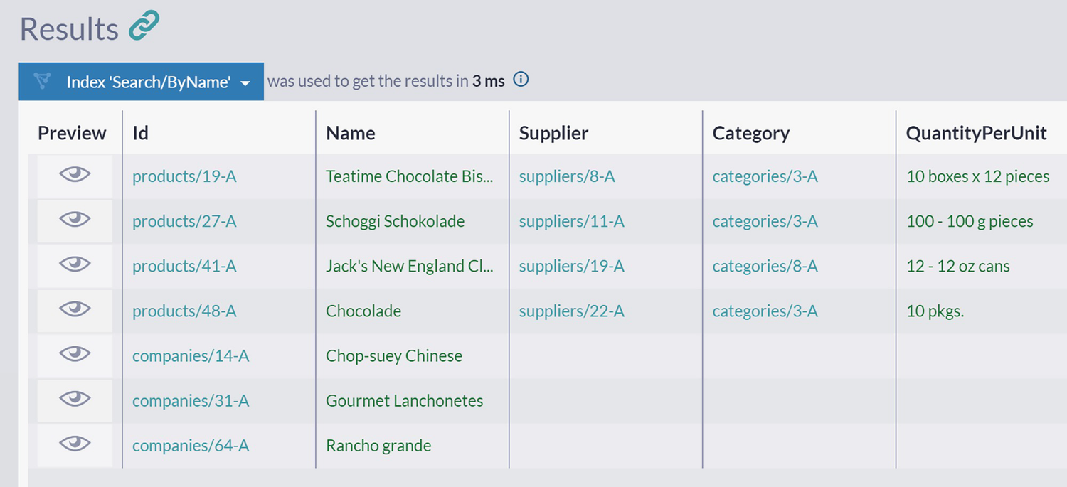
A table depicts the search results consisting of products and companies. The labeled index are preview, identification, name, supplier, category, and quality per unit.
Search Results Consisting of Products and Companies
will return products, companies, and suppliers with 3-gram ost in the Name field.
Indexing Multiple Fields from a Single Collection
It can be handy to provide a way to index (and later search) multiple properties of the documents from the same collection. When coding static indexes, you can construct an array that will hold several values. RavenDB will correctly process such arrays, creating multiple index terms per document.
Employees/ByFirstNameByLastName index
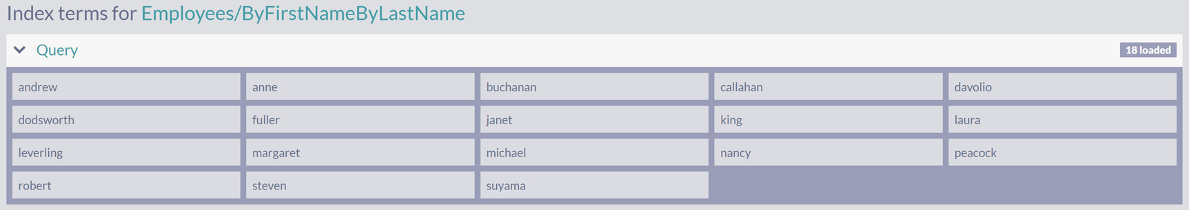
A table of the first and last names is extracted and inserted as index terms of the employees.
Indexing Terms Consisting of First and Last Names of Employees
Indexing Multiple Fields from Multiple Collections
The approach demonstrated in the previous section can be expanded further. Since you can load referenced documents during the indexing process, you can collect information from different collections to offer Omni search capabilities.
Orders/Search index
Let’s analyze this index.
Furthermore, the referenced company is loaded for every order processed, and its name is added to the query array – same for referenced employees, considering they have first and last names. Finally, we iterate over order lines, fetch their product, and load a supplier for every product, adding their names to an array .
- Order
Company
Employee
- OrderLine
Product
Supplier
We are descending three levels of references, loading referenced documents, and indexing their properties. Indexing terms will include names of companies, employees, products, and suppliers. With this index, you can search orders by various criteria.
Hence, you now have a single index that can serve queries by various criteria.
Summary
In this chapter, we covered the full-text search features of RavenDB. Besides introducing essential elements, we explained the inner workings of full-text search indexes. Finally, you learned about advanced indexing options and how to take more control over indexing with manually written static indexes.