Chapter 1

Vector Algebra

Vectors play a crucial role in computer graphics, collision detection, and physical simulation, all of which are common components in modern video games. Our approach here is informal and practical; for a book dedicated to 3D game/graphics math, we recommend [Verth04]. We emphasize the importance of vectors by noting that they are used in just about every demo program in this book.

Objectives:

    To learn how vectors are represented geometrically and numerically.

    To discover the operations defined on vectors and their geometric applications.

    To become familiar with the D3DX library’s vector math functions and classes.

1.1 Vectors

A vector refers to a quantity that possesses both magnitude and direction. Quantities that possess both magnitude and direction are called vector-valued quantities. Examples of vector-valued quantities are forces (a force is applied in a particular direction with a certain strength — magnitude), displacements (the net direction and distance a particle moved), and velocities (speed and direction). Thus, vectors are used to represent forces, displacements, and velocities. We also use vectors to specify pure directions, such as the direction the player is looking in a 3D game, the direction a polygon is facing, the direction in which a ray of light travels, or the direction in which a ray of light reflects off a surface.

A first step in characterizing a vector mathematically is geometrically: We graphically specify a vector by a directed line segment (see Figure 1.1), where the length denotes the magnitude of the vector and the aim denotes the direction of the vector. We note that the location in which we draw a vector is immaterial because changing the location does not change the magnitude or direction (the two properties a vector possesses). That is, we say two vectors are equal if and only if they have the same length and they point in the same direction. Thus, the vectors u and v drawn in Figure 1.1a are actually equal because they have the same length and point in the same direction. In fact, because location is unimportant for vectors, we can always translate a vector without changing its meaning (since a translation changes neither length nor direction). Observe that we could translate u such that it completely overlaps with v (and conversely), thereby making them indistinguishable — hence their equality. As a physical example, the vectors u and v in Figure 1.1b both tell the ants at two different points, A and B, to move north ten meters from their current location. Again we have that u = v. The vectors themselves are independent of position; they simply instruct the ants how to move from where they are. In this example, they tell the ants to move north (direction) ten meters (length).

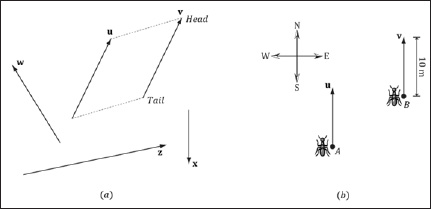
Figure 1.1: (a) Vectors drawn on a 2D plane. (b) Vectors instructing ants to move ten meters north.

1.1.1 Vectors and Coordinate Systems

We could now define useful geometric operations on vectors, which can then be used to solve problems involving vector-valued quantities. However, since the computer cannot work with vectors geometrically, we need to find a way of specifying vectors numerically instead. So what we do is introduce a 3D coordinate system in space, and translate all the vectors so that their tails coincide with the origin (Figure 1.2). Then we can identify a vector by specifying the coordinates of its head, and write v = (x, y, z)as shown in Figure 1.3. Now we can represent a vector with three floats in a computer program.

Figure 1.2: We translate v so that its tail coincides with the origin of the coordinate system. When a vector’s tail coincides with the origin, we say that it is in standard position.

Figure 1.3: A vector specified by coordinates relative to a coordinate system.

Consider Figure 1.4, which shows a vector v and two frames in space. (Note that we use the terms frame, frame of reference, space, and coordinate system to mean the same thing in this book.) We can translate v so that it is in standard position in either of the two frames. Observe, however, that the coordinates of the vector v relative to frame A are different from the coordinates of the vector v relative to frame B. In other words, the same vector has a different coordinate representation for distinct frames.

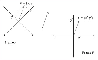
Figure 1.4: The same vector v has different coordinates when described relative to different frames.

The idea is analogous to, say, temperature. Water boils at 100° Celsius or 212° Fahrenheit. The physical temperature of boiling water is the same no matter the scale (i.e., we can’t lower the boiling point by picking a different scale), but we assign a different scalar number to the temperature based on the scale we use. Similarly, for a vector, its direction and magnitude, which are embedded in the directed line segment, does not change; only the coordinates of it change based on the frame of reference we use to describe it. This is important because it means whenever we identify a vector by coordinates, those coordinates are relative to some frame of reference. Often in 3D computer graphics we will utilize more than one frame of reference and, therefore, will need to keep track of which frame the coordinates of a vector are described relative to; additionally, we will need to know how to convert vector coordinates from one frame to another.

 

Note:    We see that both vectors and points can be described by coordinates (x, y, z) relative to a frame. However, they are not the same; a point represents a location in 3-space, whereas a vector represents a magnitude and direction. Points are discussed further in §1.5.

1.1.2 Left-Handed Versus Right-Handed Coordinate Systems

Direct3D uses a so-called left-handed coordinate system. If you take your left hand and aim your fingers down the positive x-axis, and then curl your fingers toward the positive y-axis, your thumb points roughly in the direction of the positive z-axis. Figure 1.5 illustrates the differences between a left-handed and right-handed coordinate system.

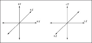
Figure 1.5: On the left we have a left-handed coordinate system. Observe that the positive z-axis goes into the page. On the right we have a right-handed coordinate system. Observe that the positive z-axis comes out of the page.

Observe that for the right-handed coordinate system, if you take your right hand and aim your fingers down the positive x-axis, and then curl your fingers toward the positive y-axis, your thumb points roughly in the direction of the positive z-axis.

1.1.3 Basic Vector Operations

We now define equality, addition, scalar multiplication, and subtraction on vectors using the coordinate representation.

    Two vectors are equal if and only if their corresponding components are equal. Let u = (u_x, u_y, u_z) and v = (v_x, v_y, v_z). Then u = v if and only if u_x = v_x, u_y = v_y, and u_z = v_z.

    We add vectors componentwise; as such, it only makes sense to add vectors of the same dimension. Let u = (u_x, u_y, u_z) and v = (v_x, v_y, v_z). Then u + v = (u_x + v_x, u_y + v_y, u_z + v_z).

    We can multiply a scalar (i.e., a real number) and a vector, and the result is a vector. Let k be a scalar, and let u = (u_x, u_y, u_z), then ku = (ku_x, ku_y, ku_z). This is called scalar multiplication.

    We define subtraction in terms of vector addition and scalar multiplication. That is, u – v = u + (–1 · v) = u + (–v) = (u_x – v_x, u_y – v_y, u_z – v_z).

Example 1.1

Let u = (1, 2, 3), v = (1, 2, 3), w = (3, 0, –2), and k = 2. Then,

    u + w = (1, 2, 3) + (3, 0, –2) = (4, 2, 1);

    u = v;

    u – v = u + (–v) = (1, 2, 3) = (–1, –2, –3) = (0, 0, 0) = 0;

    kw =2(3, 0, –2) = (6, 0, –4).

The difference in the third line illustrates a special vector, called the zero-vector, which has zeros for all of its components and is denoted by 0.

Example 1.2

We’ll illustrate this example with 2D vectors to make the drawings simpler. The ideas are the same as in 3D; we just work with one less component in 2D.

    Let v = (2, 1). How do v and –1/2v compare geometrically? We note –1/2v = (–1, –1/2). Graphing both v and –1/2v (Figure 1.6a), we notice that –1/2v is in the direction directly opposite of v and its length is 1/2 that of v. Thus, geometrically, negating a vector can be thought of as “flipping” its direction, and scalar multiplication can be thought of as scaling the length of the vector.

    Let u = (1, 1/2) and v = (1, 2). Then v + u = (3, 5/2). Figure 1.6b shows what vector addition means geometrically: We parallel translate u so that its tail coincides with the head of v. Then, the sum is the vector originating at the tail of v and ending at the head of u. (We get the same result if we keep u fixed and translate v so that its tail coincides with the head of u. In this case, u + v would be the vector originating at the tail of u and ending at the head of the translated v.) Observe also that our rules of vector addition agree with what we would intuitively expect to happen physically when we add forces together to produce a net force: If we add two forces (vectors) in the same direction, we get another stronger force (longer vector) in that direction. If we add two forces (vectors) in opposition to each other, then we get a weaker net force (shorter vector). Figure 1.7 illustrates these ideas.

    Let u = (2, 1/2) and v = (1, 2). Then v–u = (–1, 3/2). Figure 1.6c shows what vector subtraction means geometrically. Essentially, the difference v–u gives us a vector aimed from the head of u to the head of v. If we instead interpret u and v as points, then v – u gives us a vector aimed from the point u to the point v; this interpretation is important as we will often want the vector aimed from one point to another. Observe also that the length of v – u is the distance from u to v, when thinking of u and v as points.

Figure 1.6: (a) The geometric interpretation of scalar multiplication. (b) The geometric interpretation of vector addition. (c) The geometric interpretation of vector subtraction.

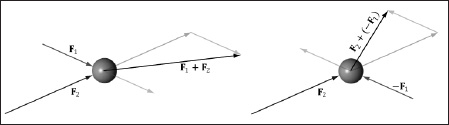
Figure 1.7: Forces applied to a ball. The forces are combined using vector addition to get a net force.

1.2 Length and Unit Vectors

Geometrically, the magnitude of a vector is the length of the directed line segment. We denote the magnitude of a vector by double vertical bars (e.g., denotes the magnitude of u). Now, given a vector v = (x, y, z), we wish to compute its magnitude algebraically. The magnitude of a 3D vector can be computed by applying the Pythagorean theorem twice; see Figure 1.8.

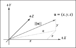
Figure 1.8: The 3D length of a vector can be computed by applying the Pythagorean theorem twice.

First, we look at the triangle in the xz-plane with sides x, z, and hypotenuse a. From the Pythagorean theorem, we have . Now look at the triangle with sides a, y, and hypotenuse . From the Pythagorean theorem again, we arrive at the following magnitude formula:

For some applications, we do not care about the length of a vector because we want to use the vector to represent a pure direction. For such direction-only vectors, we want the length of the vector to be exactly one. When we make a vector unit length, we say that we are normalizing the vector. We can normalize a vector by dividing each of its components by its magnitude:

To verify that this formula is correct, we can compute the length of $ û:

So $ û is indeed a unit vector.

Example 1.3

Normalize the vector v = (–1, 3, 4). We have . Thus,

To verify that is indeed a unit vector, we compute its length:

1.3 The Dot Product

The dot product is a form of vector multiplication that results in a scalar value; for this reason, it is sometimes referred to as the scalar product. Let u = (u_x, u_y, u_z) and v = (v_x, v_y, v_z); then the dot product is defined as follows:

In words, the dot product is the sum of the products of the corresponding components.

The dot product definition does not present an obvious geometric meaning. Using the law of cosines, we can find the relationship,

where θ is the angle between the vectors u and v such that 0 ≤ θ ≤ π (see Figure 1.9). So, Equation 1.4 says that the dot product between two vectors is the cosine of the angle between them scaled by the vectors’ magnitudes. In particular, if both u and v are unit vectors, then u · v is the cosine of the angle between them (i.e., u · v = cosθ).

Equation 1.4 provides us with some useful geometric properties of the dot product:

    If u · v = 0, then uv (i.e., the vectors are orthogonal).

    If u · v > 0, then the angle θ between the two vectors is less than 90° (i.e., the vectors make an acute angle).

    If u · v < 0, then the angle θ between the two vectors is greater than 90° (i.e., the vectors make an obtuse angle).

 

Note:    The word “orthogonal” can be used as a synonym for “perpendicular.”

Figure 1.9: On the left, the angle θ between u and v is an acute angle. On the right, the angle θ between u and v is an obtuse angle. When we refer to the angle between two vectors, we always mean the smallest angle, that is, the angle θ such that 0≤θ≤π.

Example 1.4

Let u = (1, 2, 3) and v = (–4, 0, –1). Find the angle between u and v. First we make the following computations:

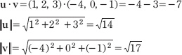
Now, applying Equation 1.4 and solving for theta, we get:

Example 1.5

Consider Figure 1.10. Given v and the unit vector n, find a formula for p using the dot product.

Figure 1.10: The orthogonal projection of v on n.

First, observe from the figure that there exists a scalar k such that p = kn; moreover, since we assumed ||n||=1, we have ||p|| = ||kn|| = |k|||n|| = |k|. (Note that k may be negative if and only if p and n aim in opposite directions.) Using trigonometry, we have that k = ||v||cosθ|; therefore, p = kn = (||v||cosθ|. However, because n is a unit vector, we can say this in another way:

In particular, this shows k = v · n, and this illustrates the geometric interpretation of v · n when n is a unit vector. We call p the orthogonal projection of v on n, and it is commonly denoted by

p = proj_n (v)

If we interpret v as a force, p can be thought of as the portion of the force v that acts in the direction n. Likewise, the vector w = v – p is the portion of the force v that acts orthogonal to the direction n. Observe that v = p + w, which is to say we have decomposed the vector v into the sum of two orthogonal vectors p and w.

If n is not of unit length, we can always normalize it first to make it unit length. Replacing n by the unit vector gives us the more general projection formula:

1.4 The Cross Product

The second form of multiplication vector math defines is the cross product. Unlike the dot product, which evaluates to a scalar, the cross product evaluates to another vector; moreover, the cross product is only defined for 3D vectors (in particular, there is no 2D cross product). Taking the cross product of two 3D vectors u and v yields another vector, w that is mutually orthogonal to u and v. By that we mean w is orthogonal to u, and w is orthogonal to v (see Figure 1.11). If u = (u_x, u_y, u_z) and v = (v_x, v_y, v_z), then the cross product is computed like so:

Figure 1.11: The cross product of two 3D vectors, u and v, yields another vector, w, that is mutually orthogonal to u and v. If you take your left hand and aim the fingers in the direction of the first vector u, and then curl your fingers toward v along an angle 0 ≤ θ ≤ π, then your thumb roughly points in the direction of w = u × v; this is called the left-hand-thumb rule.

Example 1.6

Let u = (2, 1, 3) and v = (2, 0, 0). Compute w = u×v and z = v×u, and then verify that w is orthogonal to u and that w is orthogonal to v. Applying Equation 1.5 we have,

and

This result makes one thing clear, generally speaking: u × v ≠ v × u. Therefore, we say that the cross product is anti-commutative. In fact, it can be shown that u × v = –v × u. You can determine the vector returned by the cross product by the left-hand-thumb rule. If you curve the fingers of your left hand from the direction of the first vector toward the second vector (always take the path with the smallest angle), your thumb points in the direction of the returned vector, as shown in Figure 1.11.

To show that w is orthogonal to u and that w is orthogonal to v, we recall from §1.3 that if u · v = 0, then u v (i.e., the vectors are orthogonal). Because

w · u = (0, 6, –2) · (2, 1, 3) = 0·2 + 6·1 + (–2)·3 = 0

and

w · v = (0, 6, –2) · (2, 0, 0) = 0·2 + 6·0 + (–2)·0 = 0

we conclude that w is orthogonal to u and that w is orthogonal to v.

1.5 Points

So far we have been discussing vectors, which do not describe positions. However, we will also need to specify positions in our 3D programs; for example, the position of 3D geometry and the position of the 3D virtual camera. Relative to a coordinate system, we can use a vector in standard position (see Figure 1.12) to represent a 3D position in space; we call this a position vector. In this case, the location of the tip of the vector is the characteristic of interest, not the direction or magnitude. We will use the terms “position vector” and “point” interchangeably since a position vector is enough to identify a point.

Figure 1.12: The position vector, which extends from the origin to the point, fully describes the location of the point relative to the coordinate system.

One side effect of using vectors to represent points, especially in code, is that we can do vector operations that do not make sense for points; for instance, geometrically, what should the sum of two points mean? On the other hand, some operations can be extended to points. For example, we define the difference of two points q – p to be the vector from p to q. Also, we define a point p plus a vector v to be the point q obtained by displacing p by the vector v. Conveniently, because we are using vectors to represent points relative to a coordinate system, no extra work needs to be done for the point operations just discussed as the vector algebra framework already takes care of them (see Figure 1.13).

Figure 1.13: (a) The difference q – p between two points is defined as the vector from p to q. (b) A point p plus the vector v is defined to be the point q obtained by displacing p by the vector v.

 

Note:    Actually there is a geometrically meaningful way to define a special sum of points, called an affine combination, which is like a weighted average of points. However, we do not use this concept in this book.

1.6 D3DX Vectors

In this section, we spend some time becoming familiar with the D3DXVECTOR3 class, which is the class we often use to store the coordinates of both points and vectors in code relative to some coordinate system. Its class definition is:

Note that D3DXVECTOR3 inherits its coordinate data from D3DVECTOR, which is defined as:

Also observe that the D3DXVECTOR3 overloads the arithmetic operators to do vector addition, subtraction, and scalar multiplication.

In addition to the above class, the D3DX library includes the following useful vector-related functions:

    FLOAT D3DXVec3Length(                    // Returns ||v||
        CONST D3DXVECTOR3 *pV);    // Input v

    FLOAT D3DXVec3LengthSq(                // Returns ||v||²
        CONST D3DXVECTOR3 *pV);    // Input v

    FLOAT D3DXVec3Dot(                        // Returns v₁ · v₂
        CONST D3DXVECTOR3 *pV1,   // Input v₁
        CONST D3DXVECTOR3 *pV2);  // Input v₂

    D3DXVECTOR3 *D3DXVec3Cross(
        D3DXVECTOR3 *pOut,              // Returns v₁ · v₂
        CONST D3DXVECTOR3 *pV1,  // Input v₁
        CONST D3DXVECTOR3 *pV2); // Input v₂

    D3DXVECTOR3 *WINAPI D3DXVec3Normalize(
        D3DXVECTOR3 *pOut,              // Returns v / ||v||
        CONST D3DXVECTOR3 *pV,    // Input v

 

Note:    Remember to link the d3dx10.lib (or d3dx10d.lib for debug builds) library file with your application to use any D3DX code; moreover, you will also need to #include <d3dx10.h>.

The following short code provides some examples on how to use the D3DXVECTOR3 class and four of the five functions listed above.

Figure 1.14: Output for the above program.

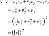
While we’re on the subject of working with vectors on a computer, we should be aware of the following. When comparing floating-point numbers, care must be taken due to floating-point imprecision. Two floating-point numbers that we expect to be equal may differ slightly. For example, mathematically, we’d expect a normalized vector to have a length of 1, but in a computer program, the length will only be approximately 1. Moreover, mathematically, 1^p = 1 for any real number p, but when we only have a numerical approximation for 1, we see that the approximation raised to the pth power increases the error; thus, numerical error also accumulates. The following short program illustrates these ideas:

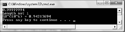
Figure 1.15: Output for the above program.

To compensate for floating-point imprecision, we test if two floating-point numbers are approximately equal. We do this by defining an EPSILON constant, which is a very small value we use as a “buffer.” We say two values are approximately equal if their distance is less than EPSILON. In other words, EPSILON gives us some tolerance for floating-point imprecision. The following function illustrates how EPSILON can be used to test if two floating-point values are equal:

1.7 Summary

    Vectors are used to model physical quantities that possess both magnitude and direction. Geometrically, we represent a vector with a directed line segment. A vector is in standard position when it is translated parallel to itself so that its tail coincides with the origin of the coordinate system. A vector in standard position can be described numerically by specifying the coordinates of its head relative to a coordinate system.

    If u = (u_x, u_y, u_z) and v = (v_x, v_y, v_z), then we have the following vector operations:

Addition: u + v = (u_x + v_x, u_y + v_y, u_z + v_z)

Subtraction: u – v = (u_x – v_x, u_y – v_y, u_z – v_z)

Scalar multiplication: ku = (ku_x, ku_y, ku_z)

Length:

Normalization:

Dot product:

Cross product:

    The D3DXVECTOR3 class is used to describe a 3D vector in code. This class contains three float data members for representing the x-, y-, and z-coordinates of a vector relative to some coordinate system. The D3DXVECTOR3 class overloads the arithmetic operators to do vector addition, subtraction, and scalar multiplication. Moreover, the D3DX library provides the following useful functions for computing the length of a vector, the squared length of a vector, the dot product of two vectors, the cross product of two vectors, and normalizing a vector:

1.8 Exercises

1.    Let u = (1, 2) and v = (3, –4). Perform the following computations and draw the vectors relative to a 2D coordinate system:

a.    u + v

b.    u – v

c.    2u + 1/2v

d.    –2u + v

2.   Let u = (–1, 3, 2) and v = (3, –4, 1). Perform the following computations:

a.    u+v

b.    u–v

c.    3u+2v

d.    –2u+v

3.    This exercise shows that vector algebra shares many of the nice properties of real numbers (this is not an exhaustive list). Assume u = (u_x, u_y, u_z), v = (v_x, v_y, v_z), and w = (w_x, w_y, w_z). Also assume that c and k are scalars. Prove the following vector properties:

a.    u + v = v + u                       (Commutative property of addition)

b.    u+ (v + w) = (u + v) + w    (Associative property of addition)

c.    (ck)u = u(ku)                   (Associative property of scalar multiplication)

d.    k(u + v = ku + kv            (Distributive property 1)

e.    u(k + c) = ku + cu          (Distributive property 2)

Hint: Just use the definition of the vector operations and the properties of real numbers. For example,

4.   Solve the equation equation 2((1, 2, 3)–x)–(–2, 0, 4) = –2(1, 2, 3)for x.

5.    Let u = (–1, 3, 2)and v = (3, –4, 1). Normalize u and v.

6.   Let k be a scalar and let u = (u_x, u_y, u_z). Prove that ||ku|| = |k|||u||.

7.   Is the angle between u and v orthogonal, acute, or obtuse?

a.    u = (1, 1, 1), v = (2, 3, 4)

b.    u = (1, 1, 0), v = (–2, 2, 0)

c.    u = (–1, –1, –1), v = (3, 1, 0)

8.    Let u = (–1, 3, 2) and v = (3, –4, 1). Find the angle θ between u and v.

9.   Let u = (u_x, u_y, u_z), v = (v_x, v_y, v_z), and, w = (w_x, w_y, w_z). Also let c and k be scalars. Prove the following dot properties:

a.    u · v = v · u

b.    u · (v+w) = u · v+u · w

c.    k(u · v) = (ku) · v = u · (kv)

d.    v · v = ||v||²

e.    0 · v =0

Hint: Just use the definition, for example,

            

10.   Use the law of cosines (c² = a² + b² = 2abcos θ, where a, b, and c are the lengths of the sides of a triangle and θ is the angle between sides a and b) to show:

            

Hint: Consider Figure 1.9 and set and use the dot product properties from the previous exercise.

11.   Let n = (–2, 1). Decompose the vector g = (0, –9.8) into the sum of two orthogonal vectors, one parallel to n and the other orthogonal to n. Also, draw the vectors relative to a 2D coordinate system.

12.   Let u = (–2, 1, 4) and v = (3, –4, 1). Find w = u × v, and show w · u = 0 and w · v = 0.

13.   Let the following points define a triangle relative to some coordinate system: A = (0, 0, 0), B = (0, 1, 3), and C = (5, 1, 0). Find a vector orthogonal to this triangle.

Hint: Find two vectors on two of the triangle’s edges and use the cross product.

14.   Prove that ||u × v|| = ||u|| ||v||sin θ. Hint: Start with ||u|| ||v||sin θ and use the trigonometric identity ; then apply Equation 1.4.

15.   Prove that ||u × v|| gives the area of the parallelogram spanned by u and v (see Figure 1.16).

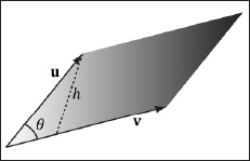
Figure 1.16: Parallelogram spanned by two 3D vectors u and v; the parallelogram has base ||v|| and height h.

16.   Give an example of 3D vectors u, v, and w such that u × v × w) ≠ (u × v) × w. This shows the cross product is generally not associative. Hint: Consider combinations of the simple vectors i = (1, 0, 0), j = (0, 1, 0), and k = (0, 0, 1).

17.   Prove that the cross product of two nonzero parallel vectors results in the null vector; that is, u × ku = 0. Hint: Just use the cross product definition.

18.   The D3DX library also provides the D3DXVECTOR2 and D3DXVECTOR4 classes for working with 2D and 4D vectors. We will later use 2D vectors to describe 2D points on texture maps. The purpose of 4D vectors will make more sense after reading the next chapter when we discuss homogeneous coordinates. Rewrite the program in §1.6 twice, once using 2D vectors (D3DXVECTOR2) and a second time using 4D vectors (D3DXVECTOR4). Note that there is no 2D cross product function, so you can skip that. (Hint: Search the index for these keywords in the DirectX SDK documentation: D3DXVECTOR2, D3DXVECTOR4, D3DXVec2, and D3DXVec4.)