Chapter 7

Texturing

Our demos are getting a little more interesting, but real-world objects typically have more details than per-vertex colors can capture. Texture mapping is a technique that allows us to map image data onto a triangle, thereby enabling us to increase the details and realism of our scene significantly. For instance, we can build a cube and turn it into a crate by mapping a crate texture on each side (see Figure 7.1).

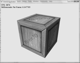
Figure 7.1: The Crate demo creates a cube with a crate texture.

Objectives:

    To learn how to specify the part of a texture that gets mapped to a triangle.

    To find out how to create and enable textures.

    To learn how textures can be filtered to create a smoother image.

    To discover how to tile a texture several times with address modes.

    To find out how multiple textures can be combined to create new textures and special effects.

    To learn how to create some basic effects via texture animation.

7.1 Texture and Resource Recap

Recall that we learned about and have been using textures since Chapter 4; in particular, that the depth buffer and back buffer are 2D texture objects represented by the ID3D10Texture2D interface. For easy reference, in this first section we review much of the material on textures we have already covered in Chapter 4.

A 2D texture is a matrix of data elements. One use for 2D textures is to store 2D image data, where each element in the texture stores the color of a pixel. However, this is not the only usage; for example, in an advanced technique called normal mapping, each element in the texture stores a 3D vector instead of a color. Therefore, although it is common to think of textures as storing image data, they are really more general-purpose than that. A 1D texture (ID3D10Texture1D) is like a 1D array of data elements, and a 3D texture (ID3D10Texture3D) is like a 3D array of data elements. The 1D, 2D, and 3D texture interfaces all inherit from ID3D10Resource.

As will be discussed later in this chapter, textures are more than just arrays of data; they can have mipmap levels, and the GPU can do special operations on them, such as applying filters and multisampling. However, textures are not arbitrary chunks of data; they can only store certain kinds of data formats, which are described by the DXGI_FORMAT enumerated type. Some example formats are:

    DXGI_FORMAT_R32G32B32_FLOAT: Each element has three 32-bit floating-point components.

    DXGI_FORMAT_R16G16B16A16_UNORM: Each element has four 16-bit components mapped to the [0, 1] range.

    DXGI_FORMAT_R32G32_UINT: Each element has two 32-bit unsigned integer components.

    DXGI_FORMAT_R8G8B8A8_UNORM: Each element has four 8-bit unsigned components mapped to the [0, 1] range.

    DXGI_FORMAT_R8G8B8A8_SNORM: Each element has four 8-bit signed components mapped to the [–1, 1] range.

    DXGI_FORMAT_R8G8B8A8_SINT: Each element has four 8-bit signed integer components mapped to the [–128, 127] range.

    DXGI_FORMAT_R8G8B8A8_UINT: Each element has four 8-bit unsigned integer components mapped to the [0, 255] range.

Note that the R, G, B, A letters stand for red, green, blue, and alpha, respectively. However, as we said earlier, textures need not store color information; for example, the format

has three floating-point components and can therefore store a 3D vector with floating-point coordinates (not necessarily a color vector). There are also typeless formats, where we just reserve memory and then specify how to reinterpret the data at a later time (sort of like a cast) when the texture is bound to the rendering pipeline. For example, the following typeless format reserves elements with four 8-bit components, but does not specify the data type (e.g., integer, floating-point, unsigned integer):

A texture can be bound to different stages of the rendering pipeline; a common example is to use a texture as a render target (i.e., Direct3D draws into the texture) and as a shader resource (i.e., the texture will be sampled in a shader). A texture resource created for these two purposes would be given the bind flags:

indicating the two pipeline stages the texture will be bound to. Actually, resources are not directly bound to a pipeline stage; instead their associated resource views are bound to different pipeline stages. For each way we are going to use a texture, Direct3D requires that we create a resource view of that texture at initialization time. This is mostly for efficiency, as the SDK documentation points out: “This allows validation and mapping in the runtime and driver to occur at view creation, minimizing type checking at bind time.” So for the example of using a texture as a render target and shader resource, we would need to create two views: a render target view (ID3D10RenderTargetView) and a shader resource view (ID3D10ShaderResource-View). Resource views essentially do two things: They tell Direct3D how the resource will be used (i.e., what stage of the pipeline you will bind it to), and if the resource format was specified as typeless at creation time, then we must now state the type when creating a view. Thus, with typeless formats, it is possible for the elements of a texture to be viewed as floating-point values in one pipeline stage and as integers in another.

 

Note:    The August 2008 SDK documentation says: “Creating a fully-typed resource restricts the resource to the format it was created with. This enables the runtime to optimize access […].” Therefore, you should only create a typeless resource if you really need it; otherwise, create a fully typed resource.

In order to create a specific view to a resource, the resource must be created with that specific bind flag. For instance, if the resource was not created with the D3D10_BIND_SHADER_RESOURCE bind flag (which indicates the texture will be bound to the pipeline as a depth/stencil buffer), then we cannot create an ID3D10ShaderResourceView to that resource. If you try, you’ll likely get a Direct3D debug error like the following:

In this chapter, we will only be interested in binding textures as shader resources so that our pixel shaders can sample the textures and use them to color pixels.

7.2 Texture Coordinates

Direct3D uses a texture coordinate system that consists of a u-axis that runs horizontally to the image and a v-axis that runs vertically to the image. The coordinates, (u, v) such that 0 ≤ u, v ≤ 1, identify an element on the texture called a texel. Notice that the v-axis is positive in the “down” direction (see Figure 7.2). Also, notice the normalized coordinate interval, [0, 1], which is used because it gives Direct3D a dimension-independent range to work with; for example, (0.5, 0.5) always specifies the middle texel no matter if the actual texture dimension is 256×256, 512×1024, or 2048×2048 in pixels. Likewise, (0.25, 0.75) identifies the texel a quarter of the total width in the horizontal direction, and three-quarters of the total height in the vertical direction. For now, texture coordinates are always in the range [0, 1], but later we explain what can happen when you go outside this range.

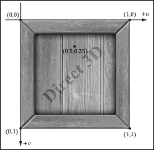
Figure 7.2: The texture coordinate system, sometimes called texture space.

For each 3D triangle, we want to define a corresponding triangle on the texture that is to be mapped onto the 3D triangle (see Figure 7.3).

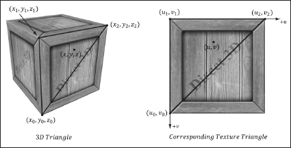
Figure 7.3: On the left is a triangle in 3D space, and on the right we define a 2D triangle on the texture that is going to be mapped onto the 3D triangle. For an arbitrary point (x, y, z)onthe 3D triangle, its texture coordinates (u, v) are found by linearly interpolating the vertex texture coordinates across the 3D triangle. In this way, every point on the triangle has a corresponding texture coordinate.

To do this, we modify our vertex structure once again and add a pair of texture coordinates that identify a point on the texture. So now every 3D point has a corresponding 2D texture point. Thus, every 3D triangle defined by three vertices also defines a 2D triangle in texture space (i.e., we have associated a 2D texture triangle for every 3D triangle).

7.3 Creating and Enabling a Texture

Texture data is usually read from an image file stored on disk and loaded into an ID3D10Texture2D object (see D3DX10CreateTextureFromFile). However, texture resources are not bound directly to the rendering pipeline; instead, you create a shader resource view (ID3D10ShaderResourceView) to the texture, and then bind the view to the pipeline. So two steps need to be taken:

1.   Call D3DX10CreateTextureFromFile to create the ID3D10Texture2D object from an image file stored on disk.

2.   Call ID3D10Device::CreateShaderResourceView to create the corresponding shader resource view to the texture.

Both of these steps can be done at once with the following D3DX function:

    pDevice: Pointer to the D3D device to create the texture with.

    pSrcFile: Filename of the image to load.

    pLoadInfo: Optional image info; specify null to use the information from the source image. For example, if we specify null here, then the source image dimensions will be used as the texture dimensions; also a full mipmap chain will be generated (§7.4.2). This is usually what we always want and a good default choice.

    pPump: Used to spawn a new thread for loading the resource. To load the resource in the working thread, specify null. In this book, we will always specify null.

    ppShaderResourceView: Returns a pointer to the created shader resource view of the texture loaded from file.

    pHResult: Specify null if null was specified for pPump.

This function can load any of the following image formats: BMP, JPG, PNG, DDS, TIFF, GIF, and WMP (see D3DX10_IMAGE_FILE_FORMAT).

 

Note:    Sometimes we will refer to a texture and its corresponding shader resource view interchangeably. For example, we might say we are binding the texture to the pipeline, even though we are really binding its view.

For example, to create a texture from an image called WoodCrate01.dds, we would write the following:

Once a texture is loaded, we need to set it to an effect variable so that it can be used in a pixel shader. A 2D texture object in an .fx file is represented by the Texture2D type; for example, we declare a texture variable in an effect file like so:

As the comment notes, texture objects are placed outside of constant buffers. We can obtain a pointer to an effect’s Texture2D object (which is a shader resource variable) from our C++ application code as follows:

Once we have obtained a pointer to an effect’s Texture2D object, we can update it through the C++ interface like so:

As with other effect variables, if we need to change them between draw calls, we must call Apply:

 

Note:    A texture resource can actually be used by any shader (vertex, geometry, or pixel). For now, we will just be using them in pixel shaders. As we mentioned, textures are essentially special arrays, so it is not hard to imagine that array data could be useful in vertex and geometry shader programs too.

7.4 Filters

7.4.1 Magnification

The elements of a texture map should be thought of as discrete color samples from a continuous image; they should not be thought of as rectangles with areas. So the question is: What happens if we have texture coordinates (u, v) that do not coincide with one of the texel points? This can happen in the following situation: Suppose the player zooms in on a wall in the scene so that the wall covers the entire screen. For the sake of example, suppose the monitor resolution is 1024×1024 and the wall’s texture resolution is 256×256. This illustrates texture magnification — we are trying to cover many pixels with a few texels. In our example, between every texel point lies four pixels. Each pixel will be given a pair of unique texture coordinates when the vertex texture coordinates are interpolated across the triangle. Thus there will be pixels with texture coordinates that do not coincide with one of the texel points. Given the colors at the texels we can approximate the colors between texels using interpolation. There are two methods of interpolation graphics hardware supports: constant interpolation and linear interpolation. In practice, linear interpolation is almost always used.

Figure 7.4 illustrates these methods in 1D: Suppose we have a 1D texture with 256 samples and an interpolated texture coordinate u = 0.126484375. This normalized texture coordinate refers to the 0.126484375 × 256 = 32.38 texel. Of course, this value lies between two of our texel samples, so we must use interpolation to approximate it.

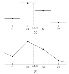
Figure 7.4: (a) Given the texel points, we construct a piecewise constant function to approximate values between the texel points; this is sometimes called nearest neighbor point sampling, as the value of the nearest texel point is used. (b) Given the texel points, we construct a piecewise linear function to approximate values between texel points.

2D linear interpolation is called bilinear interpolation and is illustrated in Figure 7.5. Given a pair of texture coordinates between four texels, we do two 1D linear interpolations in the u-direction, followed by one 1D interpolation in the v-direction.

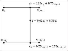
Figure 7.5: Here we have four texel points c_ij, c_i,j+1, c_i+1,j, and c_{i + 1, j + 1}. We want to approximate the color of c, which lies between these four texel points, using interpolation. In this example, c lies 0.75 units to the right of c_ij and 0.38 units below c_ij. We first do a 1D linear interpolation between the top two colors to get c_T. Likewise, we do a 1D linear interpolation between the bottom two colors to get c_B. Finally, we do a 1D linear interpolation between c_T and c_B to get c.

Figure 7.6 shows the difference between constant and linear interpolation. As you can see, constant interpolation has the characteristic of creating a blocky looking image. Linear interpolation is smoother, but still will not look as good as if we had real data (e.g., a higher resolution texture) instead of derived data via interpolation.

Figure 7.6: We zoom in on a cube with a crate texture so that magnification occurs. On the left we use constant interpolation, which results in a blocky appearance; this makes sense because the interpolating function has discontinuities (Figure 7.4a), which makes the changes abrupt rather than smooth. On the right we use linear filtering, which results in a smoother image due to the continuity of the interpolating function.

One thing to note about this discussion is that there is no real way to get around magnification in an interactive 3D program where the virtual eye is free to move around and explore. From some distances, the textures will look great, but will start to break down as the eye gets too close to them. Using higher resolution textures can help.

 

Note:    In the context of texturing, using constant interpolation to find texture values for texture coordinates between texels is also called point filtering. And using linear interpolation to find texture values for texture coordinates between texels is also called linear filtering. Point and linear filtering is the terminology Direct3D uses.

7.4.2 Minification

Minification is the opposite of magnification. In minification, too many texels are being mapped to too few pixels. For instance, consider the following situation where we have a wall with a 256×256 texture mapped over it. The eye, looking at the wall, keeps moving back so that the wall gets smaller and smaller until it only covers 64×64 pixels on screen. So now we have 256×256 texels getting mapped to 64×64 screen pixels. In this situation, texture coordinates for pixels will still generally not coincide with any of the texels of the texture map, so constant and linear interpolation filters still apply to the minification case. However, there is more that can be done with minification. Intuitively, a sort of average downsampling of the 256×256 texels should be taken to reduce it to 64×64. The technique of mipmapping offers an efficient approximation for this at the expense of some extra memory. At initialization time (or asset creation time), smaller versions of the texture are made by downsampling the image to create a mipmap chain (see Figure 7.7). Thus the averaging work is precomputed for the mipmap sizes. At run time, the graphics hardware will do two different things based on the mipmap settings specified by the programmer:

    Pick and use the mipmap level that best matches the screen geometry resolution for texturing, applying constant or linear interpolation as needed. This is called point filtering for mipmaps because it is like constant interpolation — you just choose the nearest mipmap level and use that for texturing.

    Pick the two nearest mipmap levels that best match the screen geometry resolution for texturing (one will be bigger and one will be smaller than the screen geometry resolution). Next, apply constant or linear filtering to both of these mipmap levels to produce a texture color for each one. Finally, interpolate between these two texture color results. This is called linear filtering for mipmaps because it is like linear interpolation — you linearly interpolate between the two nearest mipmap levels.

By choosing the best texture levels of detail from the mipmap chain, the amount of minification is greatly reduced.

Figure 7.7: A chain of mipmaps; each successive mipmap is half the size, in each dimension, of the previous mipmap level of detail down to 1 × 1.

7.4.2.1 Creating Mipmaps

Mipmap levels can be created by artists directly, or they can be created by filtering algorithms.

Some image file formats like DDS (DirectDraw Surface format) can stores mipmap levels directly in the data file; in this case, the data simply needs to be read — no run-time work is needed to compute the mipmap levels algorithmically. The DirectX Texture Tool can generate a mipmap chain for a texture and export it to a DDS file. If an image file does not contain a complete mipmap chain, the functions D3DX10CreateShaderResourceView-FromFile or D3DX10CreateTextureFromFile will create a mipmap chain for you using some specified filtering algorithm (see D3DX10_IMAGE_LOAD_INFO and in particular the MipFilter data member in the SDK documentation). Thus we see that mipmapping is essentially automatic. The D3DX10 functions will automatically generate a mipmap chain for us if the source file doesn’t already contain one. And as long as mipmapping is enabled, the hardware will choose the right mipmap level to use at run time.

7.4.3 Anisotropic Filtering

Another type of filter that can be used is called an anisotropic filter. This filter helps alleviate the distortion that occurs when the angle between a polygon’s normal vector and a camera’s look vector is wide (e.g., when a polygon is orthogonal to the view window). This filter is the most expensive, but can be worth the cost for correcting the distortion artifacts. Figure 7.8 shows a screenshot comparing anisotropic filtering with linear filtering.

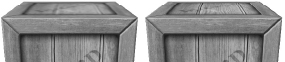
Figure 7.8: The top face of the crate is nearly orthogonal to the view window. (Left) Using linear filtering, the top of the crate is badly blurred. (Right) Anisotropic filtering does a better job of rendering the top face of the crate from this angle.

7.5 Sampling Textures

We saw that a Texture2D object represents a texture in an effect file. However, there is another object associated with a texture, called a SamplerState object (or sampler). A sampler object is where we define the filters to use with a texture. Here are some examples:

You can figure out the other possible permutations from these examples, or you can look up the D3D10_FILTER enumerated type in the SDK documentation. We will see shortly that other properties are associated with a sampler, but for now this is all we need for our first demo.

Now, given a pair of texture coordinates for a pixel in the pixel shader, we actually sample a texture using the following syntax:

As you can see, to sample a texture, we use the Texture2D::Sample method. We pass a SamplerState object for the first parameter, and we pass in the pixel’s (u, v) texture coordinates for the second parameter. This method returns the interpolated color from the texture map at the specified (u, v) point using the filtering methods specified by the SamplerState object.

7.6 Textures as Materials

In Chapter 6, “Lighting,” we specified diffuse and specular materials per vertex, with the understanding that the diffuse material would also double as the ambient material. Now with texturing, we do away with per-vertex materials and think of the colors in the texture map as describing the materials of the surface. This leads to per-pixel materials, which offer finer resolution than per-vertex materials since many texels generally cover a triangle. That is, every pixel will get interpolated texture coordinates (u, v); these texture coordinates are then used to sample the texture to get a color that describes the surface materials of that pixel.

With this setup, we need two texture maps: a diffuse map and a specular map. The diffuse map specifies how much diffuse light a surface reflects and absorbs on a per-pixel basis. Likewise, the specular map specifies how much specular light a surface reflects and absorbs on a per-pixel basis. As we did in the previous chapter, we set the ambient material to be equal to the diffuse material; thus no additional ambient map is required. Figure 7.9 shows the advantage of having a specular map — we can get very fine per-pixel control over which parts of a triangle are shiny and reflective and which parts are matte.

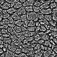
Figure 7.9: A specular map used to control the specular material at a pixel level.

For surfaces that are not shiny or for surfaces where the shininess is already baked into the diffuse map (i.e., the artist embedded specular highlights directly into the diffuse map), we just use a black texture for the specular map. Our calculations could be made more efficient by introducing a constant buffer flag and some code like this:

Thus we could skip specular lighting calculations if the application indicated it was unnecessary to perform them. However, for the purposes of our demos, we will just leave things as is, and do the calculations with a default black texture if the surface reflects zero specular light.

 

Note:    Even though our shader code works with specular maps, in this book we will not take full advantage of the per-pixel control this offers. The main reason for this is that specular maps take time to author, and should really be done by a texture artist.

7.7 Crate Demo

We now review the key points of adding a crate texture to a cube (as shown in Figure 7.1). This demo builds off of the Colored Cube demo of Chapter 5 by replacing coloring with lighting and texturing.

7.7.1 Specifying Texture Coordinates

The Box::init method is responsible for creating and filling out the vertex and index buffers for the box geometry. The index buffer code is unchanged from the Colored Cube demo, and the only change to the vertex buffer code is that we need to add normals and texture coordinates (which are shown in bold). For brevity, we only show the vertex definitions for the front and back faces.

Refer back to Figure 7.3 if you need help seeing why the texture coordinates are specified this way.

7.7.2 Creating the Texture

We create the diffuse and specular map textures from files (technically the shader resource views to the textures) at initialization time as follows:

7.7.3 Setting the Texture

Texture data is typically accessed in a pixel shader. In order for the pixel shader to access it, we need to set the texture view (ID3D10ShaderResource-View) to a Texture2D object in the .fx file. This is done as follows:

where mfxDiffuseMapVar and mfxSpecMapVar are of type ID3D10EffectShaderResourceVariable; that is, they are pointers to the Texture2D objects in the effect file:

7.7.4 Texture Effect

Below is the texture effect file, which ties together what we have discussed thus far.

One constant buffer variable we have not discussed is gTexMtx. This variable is used in the vertex shader to transform the input texture coordinates:

Texture coordinates are 2D points in the texture plane. Thus, we can translate, rotate, and scale them like any other point. In this demo, we use an identity matrix transformation so that the input texture coordinates are left unmodified. However, as we will see in §7.9 some special effects can be obtained by transforming texture coordinates. Note that to transform the 2D texture coordinates by a 4×4 matrix, we augment it to a 4D vector:

After the multiplication is done, the resulting 4D vector is implicitly cast back to a 2D vector by throwing away the z and w components. That is,

is equivalent to:

One other line of code we must discuss is:

Recall that the alpha channel of the specular map stores the specular power exponent. However, when a texture is sampled, its components are returned in the normalized [0, 1] range. Thus we must rescale this interval to a value that is reasonable for a specular power exponent. We decided on the scaling range [0, 256]. This means we can have a maximum specular power exponent of 256, which is high enough in practice.

7.8 Address Modes

A texture, combined with constant or linear interpolation, defines a vector-valued function (r, g, b, a) = T(u, v). That is, given the texture coordinates (u, v) ∈ [0, 1]², the texture function T returns a color (r, g, b, a). Direct3D allows us to extend the domain of this function in four different ways (called address modes): wrap, border color, clamp, and mirror.

    Wrap: Extends the texture function by repeating the image at every integer junction (see Figure 7.10).

    Border color: Extends the texture function by mapping each (u, v) not in [0, 1]² to some color specified by the programmer (see Figure 7.11).

    Clamp: Extends the texture function by mapping each (u, v) not in [0, 1]² to the color T(u₀, v₀), where (u₀, v₀) is the nearest point to (u, v) contained in [0, 1]² (see Figure 7.12).

    Mirror: Extends the texture function by mirroring the image at every integer junction (see Figure 7.13).

Figure 7.10: Wrap address mode.

Figure 7.11: Border color address mode.

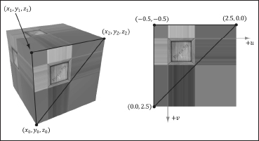
Figure 7.12: Clamp address mode.

Figure 7.13: Mirror address mode.

Since an address mode is always specified (wrap mode is the default), texture coordinates outside the [0, 1] range are always defined.

The wrap address mode is probably the most often employed; it allows us to tile a texture repeatedly over some surface. This effectively enables us to increase the texture resolution without supplying additional data (although the extra resolution is repetitive). With tiling, it is often desirable for the texture to be seamless. For example, the crate texture is not seamless, as you can see the repetition clearly. Figure 7.14 shows a seamless brick texture repeated 2×3 times.

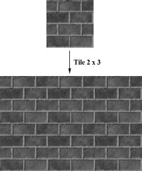
Figure 7.14: A brick texture tiled 2 × 3 times. Because the texture is seamless, the repetition pattern is harder to notice.

Address modes are specified in sampler objects. The following examples were used to create Figures 7.10 to 7.13:

 

Note:    Observe that you can control the address modes in the u and v directions independently. The reader might try experimenting with this.

7.9 Transforming Textures

As stated earlier, texture coordinates represent 2D points in the texture plane. Thus, we can translate, rotate, and scale them like we could any other point. Here are some example uses for transforming textures:

    A brick texture is stretched along a wall. The wall vertices currently have texture coordinates in the range [0, 1]. We scale the texture coordinates by 4 to scale them to the range [0, 4], so that the texture will be repeated 4×4 times across the wall.

    We have cloud textures stretched over a clear blue sky. By translating the texture coordinates as a function of time, the clouds are animated over the sky.

    Texture rotation is sometimes useful for particle-like effects; for example, to rotate a fireball texture over time.

Texture coordinate transformations are done just like regular transformations. We specify a transformation matrix, and multiply the texture coordinate vector by the matrix. For example:

Note that since we are working with 2D texture coordinates, we only care about transformations done to the first two coordinates. For instance, if the texture matrix translated the z-coordinate, it would have no effect on the resulting texture coordinates.

7.10 Land Tex Demo

In this demo, we add textures to our land and water scene. The first key issue is that we tile a grass texture over the land. Because the land mesh is a large surface, if we simply stretched a texture over it, then too few texels would cover each triangle. In other words, there is not enough texture resolution for the surface; we would thus get magnification artifacts. Therefore, we repeat the grass texture over the land mesh to get more resolution. The second key issue is that we scroll the water texture over the water geometry as a function of time. This added motion makes the water a bit more convincing. Figure 7.15 shows a screenshot of the demo.

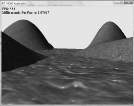
Figure 7.15: Screenshot of the Land Tex demo.

7.10.1 Grid Texture Coordinate Generation

Figure 7.16 shows an m×n grid in the xz-plane and a corresponding grid in the normalized texture space domain [0, 1]². From the figure, it is clear that the texture coordinates of the ijth grid vertex in the xz-plane are the coordinates of the ijth grid vertex in the texture space. The texture space coordinates of the ijth vertex are:

uij = j · Δu

vij = i · Δv

where

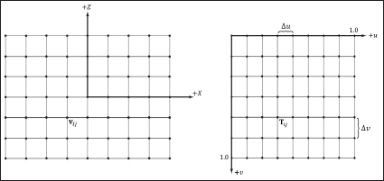
Figure 7.16: The texture coordinates of the grid vertex v_ij in xz-space are given by the ijth grid vertex T_ij in uv-space.

Thus, we use the following code to generate texture coordinates for the land mesh:

7.10.2 Texture Tiling

We said we wanted to tile a grass texture over the land mesh. But so far the texture coordinates we have computed lie in the unit domain [0, 1]², so no tiling will occur. To tile the texture, we specify the wrap address mode and scale the texture coordinates by 5 using a texture transformation matrix. Thus the texture coordinates are mapped to the domain [0, 5]² so that the texture is tiled 5×5 times across the land mesh surface:

7.10.3 Texture Animation

To scroll a water texture over the water geometry, we translate the texture coordinates in the texture plane as a function of time. Provided the displacement is small for each frame, this gives the illusion of a smooth animation. We use the wrap address mode along with a seamless texture so that we can seamlessly translate the texture coordinates around the texture space plane. The following code shows how we calculate the offset vector for the water texture, and how we build and set the water’s texture matrix:

7.11 Compressed Texture Formats

The GPU memory requirements for textures add up quickly as your virtual worlds grow with hundreds of textures (remember we need to keep all these textures in GPU memory to apply them quickly). To help alleviate memory overload, Direct3D supports compressed texture formats: BC1, BC2, BC3, BC4, and BC5.

    BC1 (DXGI_FORMAT_BC1_UNORM): Use this format if you need to compress a format that supports three color channels, and only a 1-bit (on/off) alpha component.

    BC2 (DXGI_FORMAT_BC2_UNORM): Use this format if you need to compress a format that supports three color channels, and only a 4-bit alpha component.

    BC3 (DXGI_FORMAT_BC3_UNORM): Use this format if you need to compress a format that supports three color channels, and an 8-bit alpha component.

    BC4 (DXGI_FORMAT_BC4_UNORM): Use this format if you need to compress a format that contains one color channel (e.g., a grayscale image).

    BC5 (DXGI_FORMAT_BC5_UNORM): Use this format if you need to compress a format that supports two color channels.

For more information on these formats, look up “Block Compression” in the index of the SDK documentation.

 

Note:    A compressed texture can only be used as an input to the shader stage of the rendering pipeline.

 

Note:    Because the block compression algorithms work with 4×4 pixel blocks, the dimensions of the texture must be multiples of 4.

The advantage of these formats is that they can be stored compressed in GPU memory, and then decompressed on the fly by the GPU when needed.

If you have a file that contains uncompressed image data, you can have Direct3D convert it to a compressed format at load time by using the pLoadInfo parameter of the D3DX10CreateShaderResourceViewFromFile function. For example, consider the following code, which loads a BMP file:

Figure 7.17a shows what texDesc looks like in the debugger; we see that it has the desired compressed texture format. If instead we specified null for the pLoadInfo parameter, then the format from the source image is used (Figure 7.17b), which is the uncompressed DXGI_FORMAT_R8G8B8A8_UNORM format.

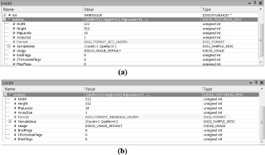
Figure 7.17: (a) The texture is created with the DXGI_FORMAT_BC3_UNORM compressed format. (b) The texture is created with the DXGI_FORMAT_R8G8B8A8_UNORM uncompressed format.

Alternatively, you can use the DDS (DirectDraw Surface) format, which can store compressed textures directly. To do this, load your image file into the DirectX Texture Tool (DXTex.exe) located in the SDK directory: D:Microsoft DirectX SDK (November 2007)UtilitiesBinx86. Then go to Menu>Format>Change Surface Format and choose DXT1, DXT2, DXT3, DXT4, or DXT5. Then save the file as a DDS file. These formats are actually Direct3D 9 compressed texture formats, but DXT1 is the same as BC1, DXT2 and DXT3 are the same as BC2, and DXT4 and DXT5 are the same as BC3. As an example, if we save a file as DXT1 and load it using D3DX10CreateShaderResourceViewFromFile, the texture will have format DXGI_FORMAT_BC1_UNORM:

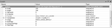
Figure 7.18: The texture is created with the DXGI_FORMAT_BC1_UNORM format.

Note that if the DDS file uses one of the compressed formats, we can specify null for the pLoadInfo parameter, and D3DX10CreateShaderResourceViewFrom-File will use the compressed format specified by the file.

Another advantage of storing your textures compressed in DDS files is that they also take up less disk space.

 

Note:    You can also generate mipmap levels (Menu>Format>Generate Mip Maps) in the DirectX Texture Tool, and save them in a DDS file as well. In this way, the mipmap levels are precomputed and stored with the file so that they do not need to be computed at load time (they just need to be loaded).

 

Note:    Direct3D 10 has extended the DDS format from previous versions to include support for texture arrays. Texture arrays will be discussed and used later in this book.

7.12 Summary

    Texture coordinates are used to define a triangle on the texture that gets mapped to the 3D triangle.

    We can create textures from image files stored on disk using the D3DX10CreateShaderResourceViewFromFile function.

    We can filter textures by using the minification, magnification, and mipmap filter sampler states.

    Address modes define what Direct3D is supposed to do with texture coordinates outside the [0, 1] range. For example, should the texture be tiled, mirrored, clamped, etc.?

    Texture coordinates can be scaled, rotated, and translated just like other points. By incrementally transforming the texture coordinates by a small amount each frame, we animate the texture.

    By using the compressed Direct3D texture formats BC1, BC2, BC3, BC4, or BC5, we can save a considerable amount of GPU memory.

7.13 Exercises

1.    Experiment with the Crate demo by changing the texture coordinates and using different address mode combinations.

2.    Using the DirectX Texture Tool, we can manually specify each mipmap level (File>Open Onto This Surface). Create a DDS file with a mipmap chain like the one in Figure 7.19, with a different textual description or color on each level so that you can easily distinguish between each mipmap level. Modify the Crate demo by using this texture and have the camera zoom in and out so that you can explicitly see the mipmap levels changing. Try both point and linear mipmap filtering.

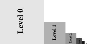
Figure 7.19: A mipmap chain manually constructed so that each level is easily distinguishable.

3.    Given two textures of the same size, we can combine them via different operations to obtain a new image. More generally, this is called multi-texturing, where multiple textures are used to achieve a result. For example, we can add, subtract, or (componentwise) multiply the corresponding texels of two textures. Figure 7.20 shows the result of componentwise multiplying two textures to get a fireball-like result. For this exercise, modify the Crate demo by combining the two source textures in Figure 7.20 in a pixel shader to produce the fireball texture over each cube face. (The image files for this exercise may be downloaded from the book’s website at www.d3dcoder.net and the publisher’s website at www.wordware.com/files/0535dx10.)

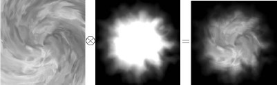
Figure 7.20: Componentwise multiply corresponding texels of two textures (flare.dds and flarealpha.dds) to produce a new texture.

4.    Modify the solution to Exercise 3 by rotating the fireball texture as a function of time over each cube face.

5.    This chapter’s downloadable directory contains a folder with 120 frames of a fire animation designed to be played over 4 seconds (30 frames per second). Figure 7.21 shows the first 30 frames. Modify the Crate demo by playing this animation over each face of the cube. (Hint: Load the images into an array of 120 texture objects. Start by using the first frame texture, and every 1/30th of a second, increment to the next frame texture. After the 120th frame texture, roll back to the first texture and repeat the process.) This is sometimes called page flipping, because it is reminiscent of flipping the pages in a flip book.

Figure 7.21: Frames of a precomputed fire animation.