This chapter will cover 3D modeling, the main feature of any three-dimensional computer graphics. Creating virtual objects gives life to an entirely new world. It is the basis for all the expressive possibilities within Blender.
We will start by creating objects and spaces, analyzing the main modeling methods. Then we will continue by learning other techniques to create three-dimensional objects, from modifiers to sculpting.
Starting in this chapter, we will develop a series of exercises that will demonstrate how to apply the techniques learned in the theoretical part.
Modeling with meshes, curves, surfaces, and other types of objects
Sculpting and the basics of modeling in Sculpt mode
Modeling with modifiers
Preparing to Start Modeling
The main feature of Blender is versatility. We can create practically every digital thing using various available modeling techniques with this software.
Unlike other software born to model only architectural objects—such as SketchUp and Autocad—or specialized in organic modelings such as Z Brush, Blender has sophisticated tools for both inorganic and organic modeling.
In version 3.0, Blender developers added essential modeling tools.
First, Geometry Nodes is a new modifier that introduces a different way of modeling. This tool was introduced in Blender 2.92. Since then, we have had many enhancements from the Blender developer team.
Mesh modeling
Sculpting
Modeling with modifiers
Modeling with armatures and simulations
Procedural modeling
We will learn about the first three techniques in this chapter and the other two in Chapter 3.
Now let’s introduce digital spaces.
Digital Spaces
Before discussing modeling techniques, we will clarify what digital space means.
Blender’s virtual space uses a Cartesian reference system and the Euclidean space.
The point is the base of Euclidean space. A set of points forms lines, planes, circles, triangles, etc. The Cartesian space provides a system of coordinates. The x-axis and the y-axis create a horizontal Cartesian plane. Joining the z-axis, vertical by convention, we define the three-dimensional space. The three axes, oriented and orthogonal, meet at a single point called origin (0.0.0). In this space, we can identify each point with its coordinates. In Blender, we deal with this space.
This world is three-dimensional and gives a precise location and size to our objects because a unit of measure establishes an accurate coordinate for each point of space.
We insert our environments and objects in this space; they are geometric elements defined by functions or algebraic equations. These objects and backgrounds are then, through render engines, transformed into images, videos, or virtual realities.
These elements are the foundation of our worlds in Blender.
Objects, materials, and lights compose a digital space. Virtual objects are Mesh, Curve, Surface, Metaball, Text Object, etc. These objects have different characteristics and details that allow us great versatility and expand our creative possibilities.
First we will learn the primary modeling techniques of Blender.
The essential tool is Mesh. Meshes have more possibilities and options than other objects; for example, some modifiers work only with meshes and not with curves or other elements.
However, as we will see later in this chapter, we can quickly transform a text or a curve into a mesh and vice versa.
Now let’s look at adding different types of objects in Blender 3.0.
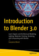
Add Objects (Shift+A)
By clicking the Add item from the Header menu or using the keyboard shortcut Shift+A, we access a window containing all the objects we can create in Blender.

The Add menu
In the first part of the window, we find the modeling objects: Mesh, Curve, Surface, Metaball, Text, Volume, and Grease Pencil.
In the second, we have two animation tools: Armature and Lattice.
In the third, we have Empty (for transformations) and Image.
In the fourth are some objects to light the scene: Light and Light Probe (support lights for Eevee).
Finally, we added Camera, Speaker, Force Field, and Collection Instance objects.
Now let’s start to analyze the different types of modeling objects we can add to our scenes.
Mesh
Meshes are the standard tools in most 3D modeling software and are composed of vertices, edges, and faces. A mesh is a grid of subobjects that defines an object in space.
In Object mode, the mesh appears as a single entity.
A vertex represents a single point in space defined by its position and three Cartesian coordinates (X, Y, Z).
An edge is a line that connects two vertices and indicates the segments common to two faces of a polyhedron, or the sides of these faces.
A face, instead, is the surface enclosed by edges and vertices. The faces can be triangles (tris), quadrilaterals (quads), or polygons with more vertices (n-gons); quadrangles are preferable to other polygons both for modeling and animation for various reasons.
These subobjects create two-dimensional or three-dimensional objects of different types: the primitives. We can modify these objects to create complex virtual forms similar to the real ones.
The following section will deal with the main modeling objects, starting from primitives, the basic geometric objects.
Add Mesh
Blender 3.0 allows us to create several basic primitives. Primitives are the primary objects of any 3D modeling software. The most basic ones are usually the same in all software.
These objects are the first geometric figures to add from the Add menu scene (Shift+A). The window that opens already contains the most common primitives; we will soon see how to add to the same window more complex objects when we need them.
Preinstalled primitives in Blender 3.0
We can add these objects: Plane, Cube, Circle, UV Sphere, ICO Sphere (the two spheres have different geometries), Cylinder, Cone, Torus, Grid (an already subdivided plane), and Susanne, the mascot of Blender.
We can modify these base shapes in Edit mode to create any desired form of them.
When we add these objects to the scene, a dialog box opens on the bottom left of the screen. We can expand it by clicking the arrow on the left.
Here, we can change the created object’s size, position, rotation, and alignment. Finally, we can collapse the dialog box by clicking the down arrow on the left.
This dialog box is available for operation only just after object creation. If we execute other commands, this dialog box vanishes. You can recall it with F9.
Let’s look at the other types of objects, starting with the Curve object.
Curve
Curves represent an essential Blender modeling object and can split into two types.
Bézier curves are mainly suitable for creating tubes, wires, bottles, glasses, texts, logos, etc.
We can also use them for other purposes, such as animated paths.
Nonuniform rational B-splines (NURBS) are more suitable for organic and beveled shapes, vehicles, and industrial design objects. Unfortunately, in Blender, this type of object has many shortcomings and is somewhat limited compared to other software such as Maya, Rhinoceros, etc.
The most crucial difference between Bézier and NURBS objects is that while Bézier objects are approximations, NURBS shapes are exact.
Both are modifiable in Object and Edit modes and composed of control points to adjust them.
The computer calculates curves faster than meshes during modeling because they contain less data, but the calculation time could be longer during rendering.
Now we see how to add and edit curves.
Add Curve

The Add Curve menu in Object mode
Bézier, an open curve
Bézier Circle, a closed circular curve
Nurbs curve, a 2D open arc
Nurbs circle, a 2D closed circular curve
Path, a 3D open curve with five aligned control points
Now let’s see the essential characteristics of Curves.
Explaining Splines
The subobject of the curve is the spline, which is composed of control points. We have three types of splines: Poly, Bézier, and NURBS.
Let’s look at them.
Poly splines are the simplest, and we do not use them to model.
We get them by converting meshes to curves, and they don’t have control points.
- Bézier splines have control points that modify their shape through a central point, a segment that crosses them tangent to the curve, and two handles at the ends, as shown in Figure 2-4.
 Figure 2-4
Bézier curves in Edit mode
Figure 2-4 shows a Bézier curve in Edit mode with various control points selected. The central point moves the segment. The two handles at the end modify the spline curvature.
The Bézier curves have four different handle types to modify the shape of the curve in various ways. We can set them either with the shortcut V or from the Object Context menu by selecting the points we want to modify, clicking with the right mouse button, and choosing the desired type in the window Set Handle Type, as shown in Figure 2-5. Figure 2-5
The Set Handle Type options of the Object context menu
In Figure 2-5, we see five options.- a.
Automatic to get the smoothest curvature
- b.
Vector to obtain sharp corners
- c.
Aligned to keep the three points in line at all times and maintain smooth curves without sharp corners
- d.
Free that creates vertices with independent handles
- e.
Toggle Free/Align, which changes the vertex from free to aligned
NURBS splines have different control points than the Bézier curves because they do not have the two handles but only the center point. Still, they have a weight option that increases or decreases the influence of the control point on the shape of the curve or surface, as shown on the right of Figure 2-6.

A NURBS in Edit mode
We can change this weight in the W Number field of the Transform panel of the Sidebar shown in Figure 2-6. If we select a point and bring the W value from 1 to 0, we see that the curve flattens, and the point no longer affects the shape of the curve. If the window is not visible, we can activate it with N.
Now we can start to modify curves.
Editing a Curve
We must create the curve in Object mode (Shift+A ➤ Curve ➤ Bézier) and then add vertices by selecting and extruding them by clicking E in Edit mode.
Finally, back to Object mode; we chose the Geometry window in the Properties Editor ➤ Object Data Properties.
Here we give shape to our curve by changing the Depth value to 0.1 in the Geometry ➤ Bevel panel.
The Toolbar
The toolbar contains the same tools for both Bézier curves and NURBS.

The Bézier curve and the toolbar in Edit mode
Here are the devices dedicated to Curves to edit them in Edit mode:
Draw outlines a freehand spline and allows us to create the curve directly, drawing fluidly without extruding one vertex at a time.
Extrude ejects new vertices from the selected existing ones.
Radius modifies the thickness of the curves by widening or tightening them at the control points.
Tilt controls the rotation of the curves.
Shear inclines selected vertices along the horizontal screen axis.
Randomize randomizes selected vertices.
We find other exciting tools in the Item window of the Sidebar that we open with N after selecting the control points we want to modify.
For example, for a Bézier curve, Radius modifies the thickness, and Tilt tilts the curve in 3D.
These tools are similar to those in the toolbar but numerically modifiable.
Object Data Properties

The Object Data Properties of the Properties Editor for Bézier curves
In Figure 2-8, in the Shape window, the first buttons, 2D and 3D, allow us to control the development of the curve and transform it from a two-dimensional to a three-dimensional object.
The default option is 3D to distribute the curve three-dimensionally in space. However, if we change the option to 2D, we keep the curve development in the two-dimensional space of the XY plane.
Resolution is an essential value because it allows us to control the definition of our curve and its smoothness: the more the value increases, the more the curve will be dense, rounded, and defined.
Thus, Resolution Preview U is the value in the 3D window, and Render U is the value for rendering.
Expanding the Geometry tab, we find various labels with their respective fields to input values.
The Extrude value allows us to extrude the curve on the z-axis, obtaining a ribbon-type shape. After that, we can choose to fill values for the Offset field. With this, we can move the curve parallel to its normal.
The Geometry window also contains the Taper object that controls the thickness of the curve along the path. For example, this tool can thin the curve toward the ends and expand it in the center.
Then, if we expand the Bevel tab, we can give a thickness to the curve modifying some value.
Round assigns a circular profile to the curve that we can control with Depth and Resolution. By changing the Resolution value, we can alter the smoothness of the angle. We also have the option Fill Caps to fill the curve caps.
The Object option allows us to add another curve to determine the profile of the primary arc. To assign the thickness, we need to add a new curve and then set it in the Object box of the Bevel window. By modifying the second curve, we interactively modify the profile of the first one.
Profile instead provides us with a tool to modify the shape of the selected curve through Depth and Resolution options. It also gives us other essential editing tools, including a graph that we can modify by changing the profile of the curve. In addition, by changing the Resolution value, we can alter the smoothness of the bevel. The options Start and End under Start & End Mapping help shorten and lengthen the curve profile, and we can create keyframes to create cool animations of the curve.
Let us now briefly introduce the Surface object.
Surface
Surfaces are the extension of curves in the three-dimensional space. Still, Blender considers surfaces and curves different entities that we cannot join into a single object.
If we create two separate meshes in Object mode, we can select them both and click Ctrl+J to join them in one object.
Instead, if we do the same thing with curves and surfaces, we can’t join them.
In Blender 3.0, the only objects we can create as surfaces are NURBS. However, if we need a Bézier surface, as we have just seen, it is possible to obtain it directly from the curve’s Object Data Properties.
To add a surface, we must use the same method for meshes and curves, from the Add menu or the shortcut Shift+A.
We have six different surfaces: NURBS Curve, NURBS Circle, NURBS Surface, NURBS Cylinder, NURBS Sphere, and NURBS Torus.
NURBS surfaces have no volume and no thickness. They are only two-dimensional objects, and they have only two interpolation dimensions. The modification systems are similar to those of curves and meshes.
Metaball is another Blender object; it is less known but no less appealing. Let’s see its primary tools.
Metaball
Metaballs are strange and simple objects defined by pure mathematical expressions directly inside Blender. Therefore, we cannot modify them in Edit mode as with meshes or curves and surfaces.
These elements influence each other, and a field of interaction surrounds them.
If Influence is positive, they will exert mutual attraction, while if it is negative, they will apply repulsion.
We can use them to create organic elements or basic shapes for natural forms. Finally, we can convert them into meshes via the Convert To button of the Object tab in the 3D View Header menu.
Object mode displays them with a black circle to select them.
While in Edit mode, they don’t have either vertices or control points but only two colored rings. The green circle allows us to adjust the stiffness, while the pink one selects the sphere and applies the main transformations.
In the Sidebar, we can change the location, the radius, and the stiffness with numerical values. In this bar, we can also change the metaball type.
Object Data Properties

The Object Data Properties of the Properties Editor for metaballs
In the Metaball window, we find the Resolution Viewport that controls the viewport visualization; the Render box determines the resolution in the render. Lowering these two values increases the resolution. Instead, the Influence Threshold option changes the influence of the entire metafamily of Metaball elements.
Objects in the same family affect each other. So to build separate entities, we need to create different families.

Changing the name and family of metaballs
We need to change the object name via the Outliner panel in the Properties Editor. Once we change the name, we create another family from this metaball.

The Active Element window
Figure 2-11 displays the Type box. Also, we have the same tools of the Sidebar. The Stiffness value controls the influence of the selected metaball. With lower stiffness values, the object is influenced and deformed by the other elements from a greater distance. Instead, the Radius value modifies the object’s size.
We now see another helpful object, Text, which is for creating logos, signs, or three-dimensional graphics and animations.
Text
The Text object is composed of mathematically calculated vector data. We use it to create two-dimensional or three-dimensional texts in which the letters are curves filled by surfaces. We write directly in Blender and make words and sentences with this tool.
We can also import text from an external text editor.
We create the Text object in Object mode. Then in Edit mode, we change the letters and write other words as in a text editor.
Finally, we can quickly transform the text into a mesh from the 3D View Header menu; select Object ➤ Convert ➤ Curve/Mesh/Grease Pencil.
Object Data Properties
As in other object cases, an essential edit box for text is the Object Data Properties of the Properties Editor, in which we find many editing tools.
On the Shape tab, we can find the standard Resolution Preview U and Render U values, which determine the resolution of the object in the 3D Viewport and in the render.
The primary text is two-dimensional, but we can give it thickness and make it three-dimensional.
On the Geometry tab, Extrude, Offset, and the other parameters are more or less similar to the Curve Object Data Properties. For example, Offset modifies the text width; Extrude extrudes the text, increasing its depth and making it three-dimensional.
We can also add a Taper object to provide a draft-like appearance such as a Bézier curve to modify the thickness.
With the Bevel tool, we can provide a chamfer feature that enhances the text’s look.
Round assigns to text a circular profile. We can control the depth and resolution. We also have the option Fill Caps.
The Object option allows us to add another object to determine the depth of the text, as with curves.
Profile instead provides us with tools to modify the text shape through the depth and resolution. It also gives us other editing tools. Moreover, by changing the resolution value, we can alter the smoothness of the bevel.
The Blender Text tool already contains many characters, and it also allows us to import external fonts.
In the Font window of the Object Data, we can click the Folder icon to load new fonts. When we click the icon, a window that contains many preinstalled typographical characters opens. In the same window, the Transform section allows us to change the dimension of our text in the Size box and the inclination in the Shear box.

Modified Blender text
In Figure 2-12, we can see the result of the default Blender text with a Bézier circle applied as a Bevel object in the Bevel window. With this operation, we have given three-dimensionality to a text. We have also changed the text’s distribution with another Bézier circle referred to as Text on Curve in the Transform window. Finally, we have converted the text into a mesh with Object ➤ Convert ➤ Mesh.
We can also assign a material to the text in the Materials window of the Properties Editor as we do with all the other objects.
After briefly discussing all the main modeling objects, let’s talk about the different elements we can add from the Add window of the main menu or with the shortcut Shift+A.
Other Blender Objects
We have seen modeling objects and the tools to modify them until now.
We can also add other kinds of objects to our scenes.
Let’s look at these: the main ones are lights and cameras to light and film our sets, or empties and images useful to help us in modeling.
Empty and Image
We begin with the Empty and Image objects.
Empty is a point in space without geometry. There are different types of empties for various purposes: Plain Axes, Arrows, Single Arrow, Circle, Cube, Sphere, Cone, Image.
We can use an empty, for example, as a reference image for modeling, or, as we will see later, to control the modifications of the modifiers, or it can be related to more objects to modify a group of them more quickly and efficiently.
We can also create an image from the menu Empty ➤ Image that opens by clicking Shift+A. In this way, an empty frame appears in the 3D view displayed in wireframe. So, we can import the image from the Properties Editor in the Object Data Properties window by loading it from the Open button of the Image window.
Instead, the Image item of the Add menu (Shift+A) allows us to import a reference image directly.
For example, we can use an image as a reference for modeling.
We can introduce an image into the 3D view both as a reference and as a background. We can also drag an image from a directory to the Blender’s 3D view already aligned with the current view.
The only substantial difference between reference and background is that while the reference image hides in the viewport the objects behind, the background is transparent.
Light
Another object that we create with the Add menu, or with the shortcut Shift+A, is Light (and Light Probe for Eevee), which we use to illuminate the scene. There are four different types of lights (point, sun, spot, and area), each with other characteristics. We will learn about lights in detail in Chapter 4.
Camera
Cameras have the characteristics of real cameras and are used to take photographs or make movies in virtual spaces.
We can add them from the Add menu or with the hotkey Shift+A.
We will see the characteristics of cameras and how to use them in Chapter 4 and throughout the book’s exercises.
This section has dealt with the main Blender 3.0 objects to create three-dimensional spaces and virtual elements. Next, we deepen our knowledge of the modeling of the primary type of object: the mesh.
Understanding Mesh Modeling
There are three modeling modes to edit a mesh: Object, Edit, and Sculpt. Object mode is the general processing way of performing the main transformations on the whole object.
Edit and Sculpt instead allow us to modify an object’s shape in subobject mode, which means acting directly on vertices, edges, and faces.
So, the Blender modeling modes are as follows:
- Object mode allows us to perform basic operations on entities as follows:
- a.
The creation of the object
- b.
The translation, rotation, and scale
- c.
The union of two or more entities
- d.
Other fundamental activities related to visualization, distribution of items in collections, etc.
We make most mesh editing operations in Edit mode by directly acting at the subobject level on vertices, edges, and faces.
Sculpt mode instead allows us to work on the mesh by sculpting it with brushes. To get good results in sculpt mode, we must have enough geometry to work efficiently with the chisels.
Object Mode

The Object items of the 3D View Header menu
Let’s look at the most important of these devices in more detail.
Transform
We can perform transformations on objects with the Transform button of the Object tab. We’ve already seen basic transformations in Chapter 1.
Set Origin
This tool sets the origin of the selected object respect to the geometry.
The origin is the orange point that Blender by default places in the object’s geometric center; it determines its location in the 3D Viewport.
It is the point of calculation of the main transformations.
Some transformations are more straightforward if the object’s origin does not match its geometric center.

The Set Origin tool of the Object menu
We can open the window shown in Figure 2-14 to move the object’s origin to the geometry, the 3D cursor, or other positions.
Mirror
We can reflect the object’s geometry by selecting the entity, clicking the Mirror button of the Object tab or with the keyboard shortcut Ctrl+M, and then pressing the Axis key of the desired transformation (X, Y, or Z).
Clear and Apply
In the Sidebar transform panel, when we create an object in the origin of the Cartesian space (0,0,0) and when this origin corresponds with the object’s origin, the location and rotation values are 0 while the scale is 1.
If we move, rotate, or scale the object, the values change with the modifications made.
Clear resets the changes we have done to the object. With this operation, we cancel the transformations, and the item returns to the original values. Also, the location and rotation values return to 0 and the scale value returns to 1 in the panel transform.
We can perform this operation by clicking Clear from the Object tab or with the keyboard shortcuts Alt+G, Alt+S, Alt+R, and Alt+O.
With the Apply button, we apply the transformations made to an object.
We do not cancel the transformations, and our object stays in the position and maintains the modified rotation and dimension.
Instead, we reset the values of the changes so that Location and Rotation return to 0 and Scale returns to 1.
We can perform this operation by clicking Apply from the Object voice or the shortcut Ctrl-A. This way we apply the main transformations: Location, Rotation, and Scale.
These two commands of the Object tab are essential when we want to animate an object or sculpt or apply modifiers or constraints. For example, in some cases, if the Scale values of X, Y, and Z are not 1, Blender does not apply some changes correctly. This error happens because it cannot interpret the object’s shape if the Scale value is not the default value of 1.
Snap

The Snap tool of the Object menu
This type of transformation snaps the selected object or the 3D cursor to a series of given points. For example, we can choose Selection to Cursor and move the center of the selected object to the 3D cursor, or Cursor to Selected and move the cursor to the center of the chosen object Cursor to World Origin, Cursor to Grid, etc.
Duplicate
We can duplicate our objects with Duplicate Objects or Duplicate Linked in the Object tab.
We create a copy of the object untied from the original by clicking Shift+D or Duplicate Objects. This duplication system is proper when, after the duplication, we want to alter one element without changing the other.
Instead, we can create a linked copy with Alt+D or Duplicate Linked. After that, if we modify one of the elements in Edit mode, we also change all the others; on the other hand, the Object mode transformations on one of the items will not alter the others.
Instead, we separate the two objects in Object mode by selecting one and clicking Object ➤ Relations ➤ Make Single User ➤ Object and Data.
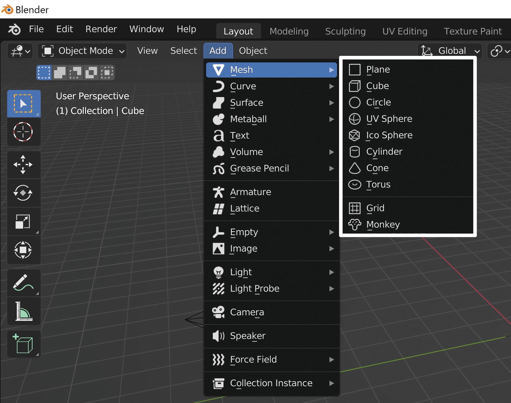
Link/Transfer Data
We can also connect separated objects by selecting them and clicking Link/Transfer Data on the Object Header's menu or with the shortcut Ctrl+L and then choosing Link Object Data in the window.
The two items remain distinct but connected, as in the previous case with Alt+D or Duplicate Linked.
Also, in this case, if we want to separate the two objects again, we can click Object ➤ Relations ➤ Make Single User ➤ Object and Data.
The Link/Transfer Data window
This can save us a lot of time. We must first select (LMB) the object where we want to copy the data, then select the second object (Shift+LMB), press Ctrl+L, and choose, in the window that opens, the data we want to copy.
Join
We can join two objects in Edit mode with the command Join or Ctrl+J. However, they must be objects of the same type; for example, we cannot merge a mesh with a Bézier curve.
If we create, with Add or Shift+A, different objects in Object mode, we build separate items.
But if we create the first one in Object mode and then select it and go to Edit mode, making the second, we create a single object.
In reverse, in Edit mode, we can separate two parts of a single object by selecting the elements to separate, pressing P, and choosing Selection in the window that opens.
Convert

Converting a mesh or a text to a curve and vice versa
In the Header menu under Object, we can select Convert and convert one object into another.
We use this tool mainly to change other objects to meshes.
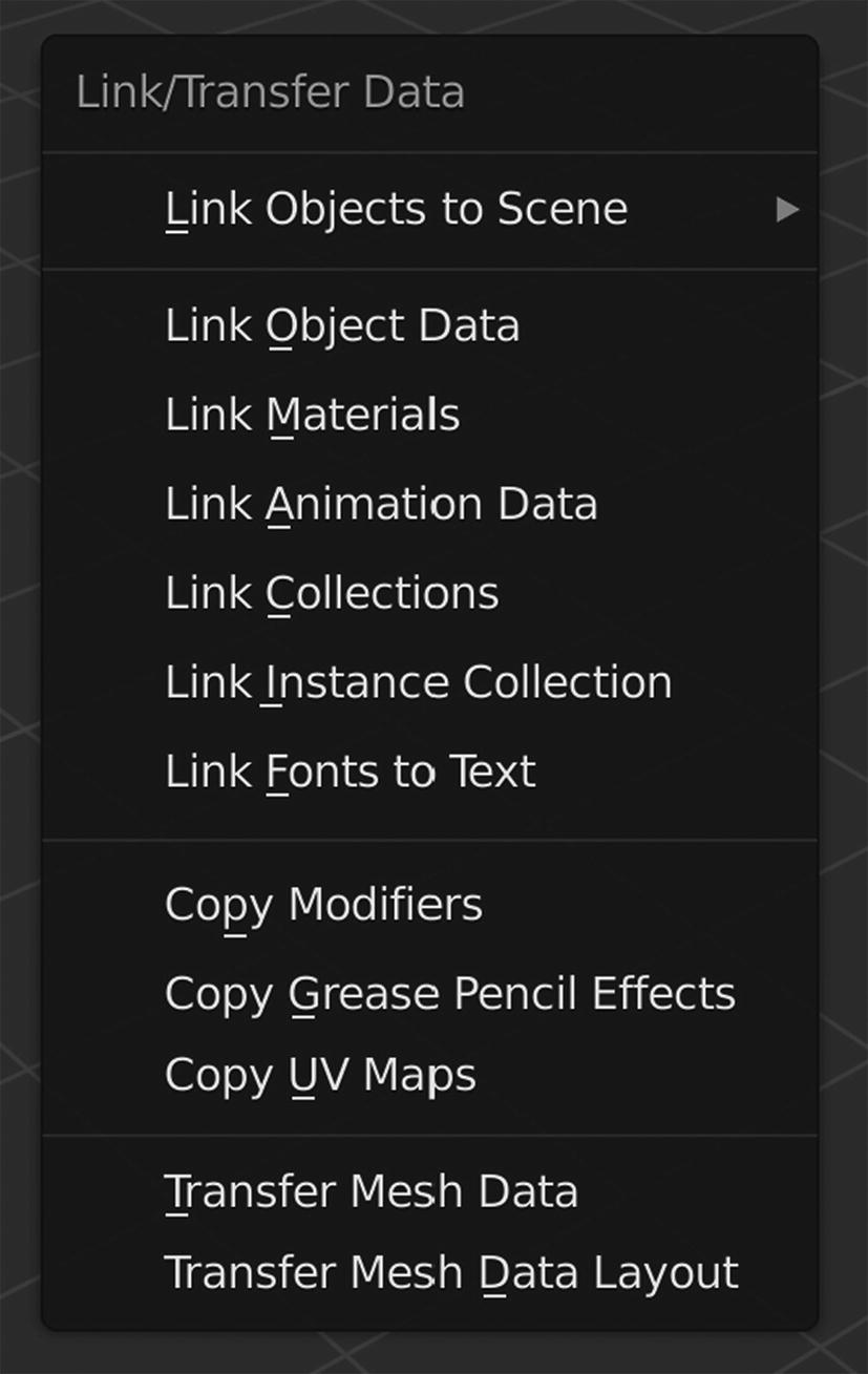
Show/Hide
If we want to work comfortably in the 3D viewport, hiding and showing some objects is essential.
The Collections display buttons
In Figure 2-18, we have highlighted the buttons Hide in Viewport, Disable in Viewports, and Disable in Renders.
For example, in an architecture project, we can separate the environment, the walls, the architectural elements, the furniture, etc., by putting them in different collections, and we can display them separately.
But there is another faster method. We can also control the display of every singular object with the Show/Hide tools. With these commands in the Object panel or with some shortcuts, we hide the selected elements of the scene.
We hide the selected objects with H; we hide the unselected things with Shift+H and show the hidden objects with Alt+H. This method is advantageous when modeling, especially when we have a scene crowded with many things.
Delete
We can delete selected objects from the scene with the command Delete or the shortcut X.
In Edit mode, we can delete vertices, edges, and faces or dissolve them, as we will see in the next session.
We have just seen the essential operations that we can perform in general in Object mode; now, let’s deepen meshes and their editing techniques in Edit mode.
Edit Mode
We can modify meshes in Object or Edit mode, as we have already seen.
We do most of the modeling work in Edit mode, where we shape our models with the many modeling tools Blender makes available.
In this modality, we create, duplicate, move, and scale objects at the subobject level with many different tools to control with the keyboard shortcuts, the 3D View Header menu, and the Object Context menu.
The subobject level involves modifying vertices, edges, and faces with their specific editing tools that we can find in the menu of the 3D view header.
Face tool menu (Ctrl+F)
Edge tool menu (Ctrl+E)
Vertex tool menu (Ctrl+V)
Before proceeding with mesh editing at the subobject level, let’s look at mesh visualization tools.
Mesh Visualization
In Edit mode, we have the tools for correct visualization of the meshes.
We must orient the face’s normals in the right way to correctly visualize an object.
Normals
Normals are the lines perpendicular to the faces. 3D modeling software uses them for the correct visualization of objects. Any 3D modeler visualizes surfaces with the normals directed toward the observer; it does not display those pointing in the opposite direction.

Displaying the normals of an icosphere
We select the object and click Tab to switch to Edit mode. Then, in the 3D View Header, we click the arrow next to the Show Overlays button, and in the window that opens, we go down to Normals and click the icon of the normal we want to display.
Normal Configuration
Normals can be reconfigured with tools and keyboard shortcuts on selected faces in Edit mode.
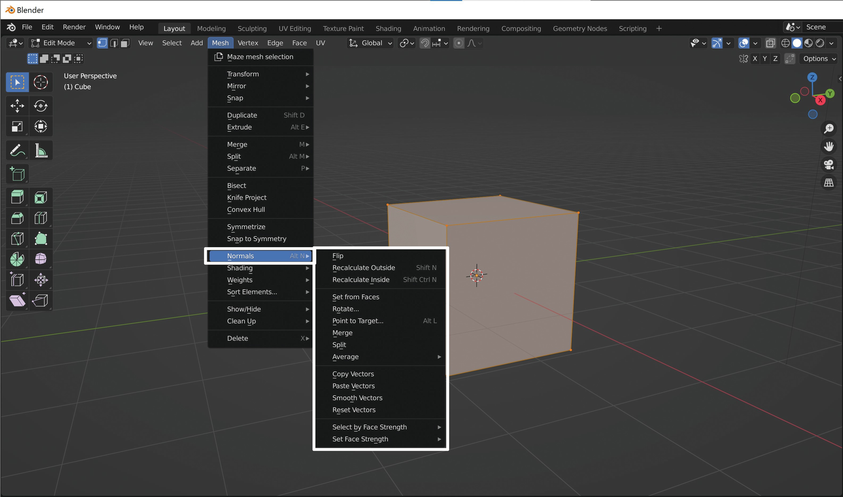
The Normals window of the 3D View Header menu
We can open the Normals window in Edit Mode, in the 3D View Header menu with Mesh ➤ Normals or the shortcut Alt+N. Here we find all the normal editing operations.
For example, with Shift+N, we can Recalculate Normals Outside, and with Ctrl+Shift+N, we can Recalculate Normals Inside. We can also use the Flip key inside the window to reverse the direction of the selected Normals.
Auto Smooth
In the Object context menu, as we saw in Chapter 1, we can choose between Shade Flat and Shade Smooth for the shading of the chosen object.
Instead, if we want to render an object with defined edges and curved parts and we have to put together flat and smooth faces, we can use Auto Smooth. We can achieve auto smoothing by selecting the objects in the 3D View. After that, we go to Object Data Properties. Then, scroll down to the Normals tab. Click the arrow to expand and select the checkbox marked Auto Smooth to enable it.
In this way, Blender automatically modifies the effect from Flat to Smooth by smoothing the edges of faces according to the face’s inclination. By default, the angle is set to 30 degrees.
Using the Angle tool in the Normals window, we can control this angle to leave the sharp corners between the faces above this value.
These results affect the visualization and not the geometry of the objects. So if we have to 3D print an object, we must change the geometry, and we can do this by adding a Bevel modifier to add more defined edges to the thing.
Now let’s see how to edit subobjects with the toolbar.
The Toolbar in Edit Mode

The first part of the toolbar in Edit mode with the main transformations
In the upper part, we have the select box. By clicking and holding down the arrow at the bottom-right corner of the button, we open a submenu that contains the various selection methods: Tweak, Select Box, Select Circle, and Select Lasso. We can choose any of these based on the requirement to select objects in 3D view.
The next button below is Cursor. We can position the cursor anywhere in the 3D view. When we click the Cursor button, its background is highlighted in different colors (depending on the selected theme). We can then left-click anywhere in the 3D view, and we can observe that the cursor goes where we click. It is super easy to place any object in a new position.
Then we have different sets of buttons, the Move, Rotate, and Scale options. With them we can move, rotate, or scale any vertex or selected set of vertices, any edge or set of selected edges, and faces or selected sets of faces. When we click and hold the mouse on the bottom-right corner of the Scale button, there is one more option: Scale Cage. We can select Scale Cage for scaling objects from a particular point or axis.
Next, we find Transform, the tool to perform the three main transformations by clicking the manipulator of the desired transformation on the 3D view. The value of this option is that we can combine all three options in one module. This thing is handy for speeding up the modeling work.

The second part of the toolbar in Edit mode
Annotate is a tool to write and draw freehand in 3D view. By clicking and holding down the arrow at the bottom-right corner of the button, we open a submenu that contains various tools for annotating: Annotate, Annotate Line, Annotate Polygon, and Annotate Eraser.
The Measure tool is also essential in geometry creation, especially in the mechanical and architectural industries. This device allows us to measure objects in the 3D view. We can clear the measurement lines by selecting one of the measured ruler ends and pressing X or Delete on the keyboard. We can also measure angles, thickness, etc.
Instead, if we click and expand Overlays in the 3D View header in Edit mode, we will find particular measurement settings such as Edge Length, Edge Angle, Face Area, and Face Angle.
Then there are other essential modeling tools:
Add Mesh allows us to add Cube, Cone, Cylinder, UVSphere, and IcoSphere objects by clicking and dragging directly on the 3D view, snapping on the grid or the object’s surface.
We have the tool Extrude to extrude vertices, edges, and faces, creating new geometry (see Figure 2-23). With the shortcuts E for extruding and Alt+E for the extruding menu, we can perform all the options of this operation. If we want to extrude a subobject, we must press E and move the mouse. We can press, for example, E ➤ Z+1 and extrude the selected object (a vertex, an edge, or a face) on the z-axis of a unit of measure. Instead, by pressing E ➤ Shift+X, we extrude on the ZY plane.

The Extrude menu (Alt+E)
After pressing Alt+E, we can see the various instruments for the Face subobject in Figure 2-23. In the Extrude menu, we find several items with different extrusion possibilities according to the selected subobject: Extrude Faces, Extrude Faces Along Normals, Extrude Individual Faces, Extrude Edges, Extrude Vertices, Extrude Repeat, and Spin.
If we want to extrude in Edit mode vertices, edges, or faces quickly, we can Ctrl+RMB click where we want the extrusion. With the same method, we can duplicate an object in Edit mode.
Another tool that adds geometry to a selected face by creating a more internal face is Inset Faces, and we can activate it from the toolbar.
Then we have Bevel, which allows us to create new geometry by inserting new loops in the selected elements by chamfering and rounding edges and corners. We can select Bevel in the toolbar and move the yellow widget that appears to create a bevel or chamfer, or we can use the shortcut Ctrl+B.
Instead we add new loops with the Loop Cut tool of the toolbar or by clicking Ctrl+R and turning the mouse wheel to increase or decrease the number of loops.
Knife and Bisect allow us to add geometry by activating the tool and cutting faces by left-clicking an edge or vertex and then dragging the mouse on another edge or vertex and clicking again. When we want to apply the modification, we have to press Enter to exit knife mode (if we’re going to leave without applying the cuts, we have to use the Esc key); passing through other edges will add vertices at the contact points between the wound and the crossed edges. The Knife shortcut is K.
Then we have Poly Build that can create meshes extruding with just the cursor’s movement. To create a shape, delete the base cube and make a plane. Then enter Edit mode, click Poly Build, and get closer to the edges or vertices; when they turn blue, we can create new faces by clicking and dragging the LMB.
Clicking and dragging the blue highlighted edge we create a face with four vertices. Instead, if we drag the mouse while pressing the Ctrl key, a unique triangular face having three vertices is created.
The ultimate tool in this part is Spin, which extrudes the selected elements (face or edge or vertex), rotating around a specific point and axis. By default, the Spin tool has no keyboard shortcut. However, we notice a dialog box appearing just below the 3D View header after pressing the Spin tool. It consists of three settings: Steps, Orientation axis X or Y or Z, and the Drag tools. With these three tools, we control the options. For example, we can select the required orientation axis during the Spin operation.
Nearby the object, we can observe a widget showing two plus signs at the ends. We can move this widget to the required position then applying the transformation.

The third part of the toolbar in Edit mode
Smooth/Randomize is the first tool in the menu from the top.
Smooth blunts the selected object, making it concave and convex.
The Randomize device instead moves the vertices of the chosen object randomly. Both tools need geometry to be effective, so if we have to apply them to the base cube, before we have to select everything in Edit mode, right-click, and subdivide the cube.
Edge and Vertex Slide move an edge loop or a group of vertices in the mesh.
Shrink/Fatten scales the selected vertices, edges, or faces depending on their normal. We can use it by choosing the required subobjects and pressing Alt+S or clicking the menu icon. After that, we can drag the mouse based on the needed scaling: shrink or inflated.
Push/Pull instead will push the selected elements (vertices, edges, or faces) closer together or pull them further apart. We open this submenu by clicking and holding down the arrow at the bottom-right corner of the of the Shrink/Fatten button. This movement occurs from the center by the same distance. We can control this distance by dragging the yellow handle up or down.
Shear and To Sphere are in the same menu, and, respectively, the first one tilts the selected subobjects along, and the second moves the selected vertices, gradually transforming the object into a sphere.
Rip Region or the shortcut V and Rip Edge, respectively, rip regions and vertices.
Now let’s look at other mesh modeling tools in Edit mode.
Other Modeling Tools in Edit Mode
The toolbar doesn’t collect all the most critical mesh editing tools at the subobject level.
We can access other tools via keyboard shortcuts or search them in the various menus.
Duplicate (Shift+D)
Just as we can duplicate objects in Object mode, we can duplicate subobjects in Edit mode from the Mesh ➤ Duplicate menu or the shortcut Shift+D.
Fill: Make Edge/Face (F)
With this tool, we create faces from already existing vertices or edges. For example, if we have three or four vertices or two already existing edges, we automatically generate a face by selecting them and clicking the shortcut F.
We can use this method also to create N-Gons, faces with more than four vertices.
However, if we have to build a face with more vertices, it is preferable to use Poly Build on the toolbar we have covered earlier in detail.
Deleting & Dissolving (X)
With these tools, we remove or dissolve subobjects. We can access them from the usual Header menu under Mesh or from a menu that appears by typing the X hotkey.
Delete cancels vertices, edges, and faces or only edges and faces and keeps vertices or deletes only faces and keeps vertices and edges.
Dissolve removes the selected elements, keeping the shape intact.
Merge Vertices (M)
We use the Merge tool to merge several vertices into one. We can access the various options from the mesh item in the header menu or shortcut M.
We have a few possibilities: At Center, At Cursor, Collapse, At First, At Last. We can choose where to put the vertex that remains with these options. For example, At First merges all the vertices with the first selected.
Then we find Merge By Distance that joins all the vertices at a certain distance from each other. We choose the length by typing the value in the Merge Distance space in the window that appears on the left side of the screen.
Separate (P)
We separate selected from unselected subobjects with this tool, creating two different objects. To operate it, in Edit mode, we choose the part of the object we want to separate and press P, choosing Selection in the window that opens. Then, in Object mode, we have two separate entities. We select them all in Object mode and press Ctrl+J to bring them together again.
Bridge Edges Loops
We use this device to connect two or more edge loops or edges across a surface, creating interconnected faces.
We can apply it from the header menu by clicking the Edge item and then clicking the Bridge Edge Loops button in the window that opens.
From the creation window on the bottom-left corner of the screen, we can also decide the number of cuts, twist the selection, and check the profile created from the Profile Factor value and the shape from profile shape.
Triangles to Quads (Alt+J)
This tool converts selected triangular faces to square faces, and we can activate it from the Header menu under Face ➤ Tris to Quads or with the shortcut Alt+J.
Now that we know about Blender’s default mesh objects, we will introduce specific mesh add-ons.
Add Mesh Add-Ons
As we saw at the beginning of this chapter, the Blender default Add menu (Shift+A) allows us to add a limited number of objects to the 3D Viewport.
From the add-ons panel of the User Preferences, we can add many more objects and, in particular, many other types of meshes to the Add menu.
We can add, for example, some shapes created directly with mathematical formulas, architectural modeling objects, or mechanical items.
If we want to add these objects to the Add menu, we have to activate the respective add-ons in the User Preferences by checking the boxes for the type of mesh we want to enable (Topbar ➤ Edit ➤ Preferences ➤ Add-ons).
There are add-ons in Blender activable in two different ways:
By enabling the preinstalled script by checking the equivalent box in the Add-ons window of the User Preferences
By downloading the installation files from the internet and clicking the install button of the User Preferences

The Add Mesh preinstalled add-ons
In Figure 2-25, we have visualized and highlighted all the Add Mesh add-ons preinstalled in Blender 3.0.
By adding these tools, the number of primitives we can create in Blender increases exponentially.
ANT Landscape (which stands for Another Noise Tool) creates landscapes and planets controllable with different parameters.
Archimesh is an architectonical tool containing many building elements, such as doors, windows, arches, columns, and walls.
The Bolt Factory allows us to create bolts and nuts with many editing options. This add-on is also handy for 3D printing. We can develop suitable screws and bolts. With this tool, we can also add a nut and a bolt to the objects we print in 3D to assemble them with other elements.
The Discombobulator enables us to modify the surfaces of an existing object and create panels for science-fiction environments.
The Extra Objects add-on is complex and adds several heterogeneous primitives collected in various groups, as we will see shortly.
The Geodesic domes add-on joins geodesic objects we can modify from a window that opens on the left of the screen at the moment of creation and controls many parameters.
Let’s take a closer look at the features of the Extra Objects, which are Add Curves: Extra Objects and Add Meshes: Extra Objects.
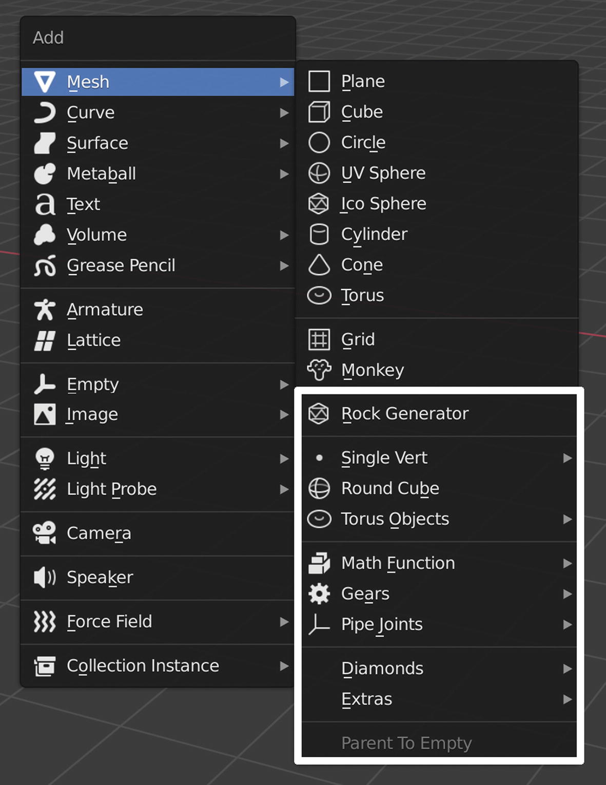
The Meshes categories of the Extra Objects add-on
The Rock Generator helps us to add easily editable rocks to the scene.
This algorithm creates an infinite variety of procedural rocks; when creating objects, a window opens on the left of the screen.
The Single Vert object adds a single vertex to the scene.
The Round Cube adds a beveled cube to the 3D Viewport.
Then we’ve got Torus objects, which adds different types of torus.
With Math Function, we add many exciting function-controlled surfaces that offer us many possibilities. We can add them by pressing Shift+A and selecting Mesh ➤ Math Function ➤ XYZ Math Surface.
With the primitive gears, we can create gear- and worm-shaped mesh objects.
With Pipe Joints, we can add different types of pipes, pipe joints, or tubes with angles.
The Diamonds menu adds diamond-shaped meshes.
The Extras menu adds several exciting objects, such as Wall Factory, that allows us to create stone or brick walls but has many options that we can use to create surreal and science-fiction sets.
Finally, we have Parents to Empty, which adds an empty as a parent of the selected mesh.
Many external add-ons can be downloaded from the Internet and installed in Blender. Some of these are free; for others, we have to pay small amounts.
We can find many of them on this site:
https://blender-addons.org/advanced-boolean-tool-abt-addon/
In Chapter 3, we will study other interesting mesh editing add-ons such as Edit Mesh Tools, Bool Tool, etc.
After learning more about the main mesh modification methods in Object mode and Edit mode in this section, we go on with a completely different and more intuitive modeling system: sculpting.
Sculpting
Sculpting is a modeling system much more intuitive than that studied until now.
It is a potent tool that already allows us to obtain professional results and that the Blender Foundation is continuing to develop.
In Edit mode, we work with technical and specific tools at the subobject level.
In Sculpt mode, we model with brushes on a very dense mesh, changing the topology directly. Indeed, we need a lot of vertices to sculpt our objects.
We model like in reality: we shape a sculpture with virtual materials such as clay.

The interface of Blender 3.0 in Sculpt mode
On the left, in the toolbar, we have all the brushes or chisels, masks, and tools for the main transformations. The cursor turns into a brush represented by a blue, red, or yellow circle depending on the chisel type.
Also, the Tool Settings on the top of the 3D view, the toolbar, and the Active Tool and Workspace Settings panel of the Properties Editor allow us to modify the characteristics of brushes, masks, and tools inherent to the virtual sculpture.
In digital modeling, we use virtual chisels to edit shapes like working with real instruments; let’s see more closely what they are and how they work.
Brush Settings
Sculpt mode has many features in Blender 3.0. This digital modeling system is becoming more and more critical in open source software like Blender.
Let’s start to model.
It is essential to have a pen tablet for painting, sculpting, and drawing because, with the pen, we can control the brush more efficiently, even with tip pressure.
First, we must distinguish between tools and brushes. The tools are on the toolbar and have general settings; instead, brushes are our tools saved with the customized settings. We can keep our brushes and find them on the Tool Settings of the 3D View header. We create our brushes based on the tools present by default.
We build our own set of brushes starting from the existing ones, modifying their characteristics, and then saving them in the Properties Editor’s Active Tool and Workspace Settings tab.
So, we select the desired brush in the toolbar, click the Add Brush button in the Active Tool and Workspace Settings tab, and name it. Finally, we modify its characteristics in the Tool Settings of the header of the 3D Viewport.
We can find it whenever we need it in the window that opens by clicking the Browse Brush button in the Tool Settings.
The cursor turns into a brush represented by two circles in Sculpt mode. The smaller circle depicts the force, and the larger one displays the radius. The dot represents the point of action.
The default chisel is Draw, which moves outward vertices within the brush radius.
Holding Ctrl, we obtain the opposite effect pushing the affected vertices inward; instead, we smooth the vertices and flatten the surface holding down Shift.
By pressing F, we scale the dimension of the brush, and by pressing Shift+F, we change the strength of the tool. We can obtain the same result with the Radius and Strength values in the Settings tool of the 3D Viewport header.
In the Active Tool and Workspace settings window of the Properties Editor, we can find all the values to modify the characteristics of the selected brush: Radius, Strength, Direction, Normal Radius, Hardness, and Autosmooth.
Now let’s start modeling some simple shapes.
Preparing the Object
We can start modeling quickly by creating a new file from the Topbar menu by selecting File ➤ New (Ctrl+N) and choosing Sculpting from the drop-down menu.
We are in the Sculpting workspace with a spherical object ready to sculpt.
This way is the quickest to start modeling.
But we can create shapes to model with several other methods.
We can build any primitive and subdivide it to add vertices.
We can model the general shape with several separate primitives in Object mode and join Ctrl+J in a single mesh to create a more complex object. Of course, meshes must have closed forms. We can also use the Boolean modifier, as we will see later in this chapter.
Then we go to Sculpt mode and add more and more details to model more organic shapes. So, let’s create our form. We start with a cube and switch to Edit mode with Tab.
Then we right-click the object to open the Object context menu. In the Object context menu window, we click Subdivide to create more geometry; we change the number of cuts to 40 and increase the Smoothness value to 1.00.
Let’s go back to Object mode, right-click the smoothed Cube, and choose Shade Smooth. Then we add a Subdivision Surface modifier to our object and set Levels Viewport and Render values to 2.
Then we apply the modifier.
We can also use the Multiresolution modifier and set the number subdivision to 3.
Please see the “Modeling with Modifiers” section of this chapter to see how they work.
If we want to change the scale of our element, enlarging or shrinking it, it is essential to apply the transformation with the shortcut Ctrl+A and then select Apply ➤ Scale.
This shape is my favorite, ready to sculpt everything, starting from a smoothed cube.
We have prepared the object to model. Now we set the interface to sculpt.
Preparing the Interface
We can switch directly to the Sculpting workspace, already set for this type of modeling.
Let’s set the toolbar as a dual-column row to have all the instruments available simultaneously in the interface. When the mouse is on the right edge of the toolbar, a double-sided arrow appears. If we click the left mouse button and move it to the right, we arrange the instruments in two vertical lines. If we continue to drag the mouse, the name will be displayed next to the brush.
We find the Properties Editor’s Active Tool and Workspace Settings to the right of the interface.
Now we’re ready to sculpt, and we can learn about Blender’s various digital sculpting tools.
Sculpting Tools
Let’s look at the essential modeling tools of Blender’s Sculpt mode. We have many instruments available, divided into a few categories and identified by the color assigned to them in the interface.

The toolbar in Sculpt mode with the Blue tools
These are the essential tools of Sculpt mode that add or subtract volume; let’s look at them one by one:
Draw (X) is the default brush that moves the vertices inward or outward following the vertices’ normals. You have to press Ctrl to dig the surface instead of extruding it.
Draw Sharp digs into the surface and is essential to define the details; it acts more precisely than Draw, with a sharper falloff to delineate the shape exactly. By pressing Ctrl, we reverse the effect, and we rise vertices up from the volume. In other words, since this is more precise than Draw, we can consider this as a finishing operation during sculpting.
Clay (C) is similar to Draw but smoother and more precise in defining the plans. It looks like modeling clay, but virtual clay. This tool combines the Draw brush with the Flatten brush.
The Clay Strips brush is similar to clay but with more defined brushstrokes. The effect is like modeling with a flat shape rather than the more rounded Clay chisel shape.
Clay Thumb is another tool that we can use to reproduce digital modeling. It creates fingermarks on the surface, like when you model natural clay with your thumbs.
The Layer brush (L) creates flat surfaces extruded from the base surface and generates several overlapping surface layers. As long as we hold down the left mouse button to sculpt, it extrudes a single surface, while when we interrupt and resume a new session, this brush resets and creates a new layer.
Inflate (I) inflates the sculpted surfaces softly and irregularly. This instrument is similar to Draw but softer and more rounded.
The Blob brush acts like Inflate, creating more decisively spherical surfaces. It also allows controlling the connection points between the existing surface and the spherical surfaces it makes.
Crease (Shift+C) creates square indentations by digging the mesh.

The toolbar in Sculpt mode with the Red tools
Smooth (S) blunts the surfaces and flattens the irregularities, making the shape softer and smoother.
Flatten (Shift+T) flattens the volume by setting an average height between the vertices of the area of influence. When using Ctrl when working, we reverse the effect and increase contrast.
The Fill brush acts as the flatten brush by flattening the surfaces, but more decisively, and by filling holes or grooves between them. When using Ctrl instead, we increase the surface contrasts and define more precisely the details.
Scrape flattens the surface leaving a mark similar to that of clay modeling spatulas. In addition, it increases the contrasts of hollowed-out parts.

The toolbar in Sculpt mode with the Grab tools
Multiplane Scrape scrapes the mesh surface with two inclined planes, creating an angle with a sharp edge in the center. The Plane Angle option increases the angle between the two planes, making it brighter and more defined. Holding Ctrl reverses the corner.
Pinch (P) brings the vertices closer to the center of the brush. Pressing Ctrl activates the option Magnify that moves vertices away.
Grab (G) does not add vertices to the shape but drags the existing ones in the direction of the mouse pointer.
Elastic Deform is similar to Grab but smoother and softer in dragging the vertices while maintaining a regular shape.
Snake Hook (K) is similar to Grab but creates more defined and thinner shapes. It pushes the form in the direction of the brush and allows us to develop snake-like forms.
Thumb is similar to Grab but with flatter and thinner surfaces. It flattens the mesh by moving it in the direction of the cursor.
Pose moves the selected part of the mesh as an armature. Blender calculates the point of rotation considering the dimension of the brush. By clicking Ctrl during the transformation instead of the rotation movement on the pivot, the selected shape rotates perpendicularly to the form itself in the direction of the mouse movement.
Nudge rotates the vertices in the direction of the mouse movement.
Rotate, like Nudge, rotates the vertices in the direction of the mouse movement in a much more defined and accentuated way to create vortices.
Slide Relax flows the mesh’s topology in the direction of the mouse movement, trying to preserve its volume. This tool enters the Relax mode by pressing Shift and creates a more uniform distribution of the faces without deforming the mesh volume.
Boundary modifies the mesh contours according to the options in the Deformation drop-down menu of the Brush Settings window of the Active Tool and Workspaces Settings: Bend, Expand, Inflate, Grab, Twist and Smooth.
Cloth allows us to simulate cloth physics interactively on the mesh we are editing. It mimics fabric folds. It is preferable to use brushes of small size.
To use the Simplify brush, we must activate dynamic topology. This tool simplifies the geometry concerning detail size in the Dyntopo window.
Mask (M) is an essential tool. It allows us to mask the mesh parts not to change the brushes. The mask is represented in 3D view by grayscale tint. To select the parts we don’t want to edit, we must paint them dark gray. The lighter parts will remain editable with the tools. Holding Ctrl we change the brush into an eraser and clicking Shift with Mask we switch to Mask smoothing mode.
To deactivate the mask, we must press Alt+M or paint with the same tool selecting the minus sign (-) in the Header Tool Settings of the 3D Viewport. By pressing Shift with the Mask tool active, we switch to smoothing mode.
Multires Displacement Eraser erases changes made in the offset of a sculpted object. To get an effect, we need to apply a Multiresolution modifier and then modify the object’s shape with other brushes before acting with this tool.
Multires Displacement Smear modifies the offset of a sculpted object.
To get an effect, we need to apply a Multiresolution modifier and then vmodify the object’s shape with other brushes before acting with this tool.
Draw Face Sets modifies the visibility of the mesh by changing the color of the selected faces every time we click the left mouse button. We use it, as we will see shortly, with Edit Face Set.

Mask, Hide, Filter, and other Blender 3.0 sculpt tools
Box Mask, Lasso Mask, and Line Mask give us different masking possibilities to prevent object modification.
Box Hide hides the mesh parts we click and drag with the left mouse button; of course, the tools do not modify them. Then, with Alt+H, we bring everything back into view.
Box Face Set and Lasso Face Set are the same as Draw Face Sets, but while the latter has a brush painting mode, the first ones have methods of selecting the faces to be painted by Box and Lasso.
Box Trim and Lasso Trim allow us to cut the object with Box and Lasso modes.
The Line Project tool cuts the object following a straight line. We draw this segment by clicking and dragging the cursor in the 3D viewport. The shady part of the mesh is cut off.
Mesh Filter applies a deformation to the entire object through a filter.
We can choose different filters in the Tool Settings or the Active Tool and Workspace Settings panel.
Filters in Blender 3.0 include Smooth, Scale, Inflate, Sphere, Random, Relax, Relax Surface Sets, Surface Smooths, Sharpen, Enhance Details, and Erase Displacement.
These filters modify the shape by applying their algorithm to the whole object; for example, Smooth smooths the form, and Inflate expands it.
Cloth Filter applies the same modifications as the Cloth brush to the whole object.
We use the Edit Face Set tool with Draw Face Sets, Box Face Set, or Lasso Face Set. This tool modifies selections made with the previous tools by enlarging them, shrinking them, etc. It currently provides the following devices: Grow Face Set, Shrink Face Set, Delete Geometry, Fair Positions, and Fair Tangency. We find them in the Properties Editor’s Active Tool and Workspace Settings panel.
Finally, we have the standard tools for the main transformations: Move, Rotate, Scale, and Transform, followed by the Annotate tool group.
Now let’s see how to work on a mesh by adding geometry with different tools.
Adding Resolution
The Multiresolution modifier adds geometry to the mesh by making it denser. This tool is not specifically for Sculpt mode, but we can use this modifier effectively when sculpting.
Remesh is useful when we want to standardize the level of detail of our objects and decide their density.
The Dynamic Topology option adds and removes details interactively while we work.
In the next section of this chapter, dedicated to modifiers, we will see the Multiresolution modifier.
Next, we will learn about two systems to make a denser polygons mesh, dedicated expressly to the Sculpt mode: remesh and dynamic topology.
Remesh
We apply Remesh to the object after the sculpting. We can achieve uniform geometry and modify its density as we like.
Dynamic Topology instead is interactive and allows us to add geometry in the exact moment we sculpt.
These tools are effective and will enable us to define details of the modeled object as we want.
We can start from a basic shape created with other sculpting techniques.
In this case, we can combine different primitives to form a primary object and then go into Sculpt mode.
When we want to standardize the geometry of different shapes or increase the mesh density to edit it into sculpt mode, we can use Remesh.
Of course, this tool will not work if we have Dyntopo active simultaneously.

The Remesh options
We access the Remesh window from the Remesh button in the Tool Settings of the header of the 3D window, and we click the Remesh button.
This way, we create a mesh from the geometry with a correctly distributed topology without any shape change.
Editing the object in Sculpt mode, we move the vertices and modify the mesh’s geometry. For example, using the grab brush, we drag the vertices. Then, switching to edit mode, we see that the mesh is less dense where we have worked with this brush because sculpting has moved the vertices away. Remesh helps us make the geometry of our object more homogeneous, retopologizing and unifying the density of the vertices.
Dyntopo
Dynamic topology is interactive and helps us create new geometry when we need it while sculpting.
So, we don’t have to start from a high-defined mesh in this case.
We add geometry and change the object’s topology during the sculpting. Thus, we can model interactively without adding too much geometry to the base object when we activate this tool.

The Dyntopo options
We can toggle Dyntopo with the checkbox in the Tool Settings, as we have just seen, or with the Ctrl+D shortcut.
Most brushes will subdivide the mesh with dynamic topology active during the stroke.
We have seen how to sculpt with Blender 3.0 and interactively with Dyntopo; now, let’s see how to model by applying different algorithms to objects: the modifiers.
Modeling with Modifiers
Modifiers are an essential part of Blender’s structure and involve different software functions, from modeling to animation to physics.
They are efficient modeling tools in many cases.
They are separate algorithms applied to objects that are not directly part of the object and modify the mesh, so we assign them nondestructively.
So we can modify the object by changing the modifier values at any time. We can apply them when we have obtained the desired result or delete them if we decide they are not necessary. If we delete the modifier, we cancel every effect exerted on the object.
We can add to a single object all the modifiers required with different functionalities until we obtain the desired result. If we want to apply the modifiers all at once, we can do so from 3D view’s header menu by selecting Object ➤ Convert ➤ Mesh.

The header of the Modifier Properties window in the Properties Editor
In Figure 2-34, we can see the following:
The Add Modifier button. It allows us to choose and add the modifiers.
The modifier stack. It is the list of all modifiers applied to that object. If we have added multiple modifiers, we can reorder them as per our requirements before applying them.
The three buttons to display the modifier in Edit mode, Viewport, and Render mode.
Next to the buttons, we see the arrow that opens the menu to apply, duplicate, and move the modifier in the modifier stack.
With X, we can instead delete the modifier to cancel the modifications from the object.
We add each new modifier at the bottom of the list; the changes performed by modifiers are calculated from top to bottom.
We can modify their position so that each time we get the layout we need.
For example, if we want a reflected and smoothed shape, we must have the mirror modifier at the top of the stack for a correct effect.

Blender’s modifiers
The Modify category checks the object’s data. For example, the Data Transfer modifier transfers data from one mesh to another.
The Generate group creates new geometry or modifies the existing one. For example, the Mirror modifier mirrors the mesh, or the bevel modifier smooths the angles of the objects by adding new edges.
The Deform group modifies the object’s shape without changing the object’s geometry or creating new geometry.
The Physics category groups the modifiers that affect the physical effects, and Blender automatically adds them when applying a physical simulation to an object.
This chapter will only discuss some of the modifiers useful for object modeling.
However, Blender supports several other modifiers for modeling and many other functions.
But let’s take a closer look at the ones we are most interested in for modeling.
Generate Modifiers
As we’ve just said, there are four groups of modifiers.
In this chapter, we deal with two types: Generate and Deform. These categories are the most suitable for modeling.
We will look at the Geometry Nodes modifier, which Blender 3.0 implemented to edit objects’ geometry and create procedural modeling.
Let’s start with the Generate modifiers, adding geometry to the object or modifying it significantly.
Array
We can use the Array modifier to create groups of objects to develop complex scenes with repeated elements.
It builds an array of copies of one element.
We can determine the number of instances with the Count value. Then, we can shift them with an offset determined as Relative Offset or Constant Offset.
We can also move, rotate, or scale the array concerning a reference object with the Object Offset option.
The reference object can be an empty, and we must choose it in the Object Offset box. This empty replaces the offset table’s numerical values. It controls the transformations series of objects reproduced by the modifier, so it is sufficient to translate, rotate, or scale this object to modify the arrangement of the repeated elements in 3D view.
We can also add more than one array modifier to the same object to multiply the element with different spatial distributions on the various Cartesian planes.
By selecting Merge, we merge the vertices of each copy according to the Distance value; also, selecting First Last, we join the vertices of the first with those of the last if they are in the distance range we set.
Bevel
The Bevel modifier bevels the edges of the object and allows us to control the width type of the angle, the amount or percent, and the number of segments. We can also modify the bevel shape with the Profile option.
We have five options that control width types: Offset, Width, Depth, Percent, and Absolute.
If we click the Vertices button, the effect is applied only to the vertices and not the edges.
At the same time, under Geometry tab intersections, Clamp Overlap prevents new geometries from intersecting and overlapping the existing ones.
By changing the Profile value, we modify the shape of the beveled profile.
We can choose between a default profile and a customizable one.
Miter Outer and Inner are functional in the Geometry window when two beveled edges meet at an angle. Still, one last important option in the same window is Intersection Type that controls the intersections at the vertices. It can be adjusted as Grid Fill to maintain a smooth continuation of the bevel profile or Cutoff that creates a cutoff face at the vertices.
Several other options allow us to solve even the most complex cases that we won’t see in this book.
Boolean
The Boolean modifier is a simple-to-use tool that combines two objects to create a single entity with the possibility of making the two meshes interact in three ways: Intersect, Union, and Difference.
With the first operation, we keep the intersection of both objects. With the second, we obtain the union of both meshes in a single element.
With the third operation, we subtract from the first object the part in common with the second.
We can also apply the modifier to more than one object simultaneously by choosing a collection as an operand type instead of just one entity.
Let’s see how to use this modifier.
We need two meshes: select the first one, add Boolean from the modifier stack, and choose one of the three available interaction types. Then we add the name of the second object in the Object box or click it with the eyedropper.
We must select Wireframe for the objects in the Viewport Display section of the Object Properties window to see the geometry changes in real time. To better view the creation process, we can also enable Toggle X-Ray.
Once we finish this operation, applying the modifier and deleting the second object is essential because Blender does not automatically delete it.
In many cases, it is convenient to replace this modifier with the Bool Tool add-on.
With this add-on, we can directly edit objects, simplifying the application process. We will see this tool in Chapter 3.
Decimate
The Decimate modifier allows us to reduce the number of polygons of an object as much as possible without changing its shape. We use it, for example, to simplify the geometry of objects modeled in Sculpt mode. But, too exaggerated reductions can also heavily modify the object’s geometry until it is unrecognizable.
The Collapse feature combines the vertices progressively, and the value that controls the changes is Ratio. The value 1.0 keeps the original mesh, while 0 annihilates the geometry.
Un-subdivide is more or less the opposite of Subdivide that we have seen among the mesh editing tools to add geometry to the object. Therefore, we must use it mainly for meshes with grids-based topology.
Planar is particularly useful on shapes composed mainly of flat surfaces. The value to reduce the geometry is Angle Limit, where we can choose the angle to minimize the geometry.
At the bottom of the window, there is the Face Count setting, which is the number of faces after the reduction.
Geometry Nodes
This is a fundamental tool for creating and modifying geometry and procedural modeling. So, we can’t help but dwell a little bit longer on it.
The Geometry Nodes modifier has been part of Blender since version 2.92 in early 2021, and new nodes have been added continuously since then.
Now in Blender 3.0, we are starting to see the first results.
It’s a complex system that is getting bigger and bigger, and in this book, we only have time to introduce the basic concepts.
This modifier allows gathering, through a nodal system, all the Blender modifiers to edit the object’s geometry.

The Geometry Nodes workspace
At the top of Figure 2-36, we see the button for activating the Geometry Nodes workspace. This workspace comprises the Spreadsheet Editor on the top left, the 3D Viewport, and the Geometry Nodes Editor at the bottom, highlighted by the white box. Then, as usual, there are the Outliner and the Properties Editor on the right.
At the top of the Geometry Nodes Editor, there is the button New to create the nodal system and some nodes to create the simple object that we can see in the 3D Viewport.
The Group Input and Group Output nodes appear in the Geometry Nodes Editor by clicking the New button.
In addition, a Geometry Nodes modifier appears in the Modifier Properties of the Properties Editor.
In this case, we have applied a Point Distribute node to the cube to distribute points on its surface. The Join Geometry node allows us to visualize the cube and the distributed elements togheter.
The points and their distribution in space are the fundamentals for the geometry nodes.

The Cube vertices in the spreadsheet
The geometry nodes modifier works on this information.
- 1.
Open Blender and create a new file.
- 2.
Select the Geometry Nodes workspace in the Topbar to open the nodal modeling interface.
- 3.
Delete the default cube and create a plane (Shift+A ➤ Mesh ➤ Plane). Then, scale the plane (S ➤ 4) and apply the transformation (Ctrl+A ➤ Scale).
- 4.
Create a new modifier by clicking the New button in the middle of the Geometry Node Editor window. Then, a Geometry Nodes modifier appears in the Modifier tab of the Properties Editor.
You can also add the modifier directly from the modifier panel of the Properties Editor by clicking Add Modifier and then on Geometry Nodes in the section “Generates.”
- 5.
Add a Point Distribute node (Shift + A ➤ Search ➤ Point Distribute), distributing points on the plane’s surface and creating a cloud of points instead of the plane itself. These points are displayed in the spreadsheet, as shown in Figure 2-38.

The Point Distribute node
- 1.
In the Topbar, select the Geometry Nodes workspace.
- 2.
Create a new modifier by clicking the New button in the middle of the Geometry Node Editor window.
- 3.
Let’s delete the Group Input node and add an IcoSphere node from the Mesh Primitives menu to create a primitive object and connect it with the Group Output node.
- 4.
By adding a Transform node from the Geometry menu and inserting it between the two existing nodes, we can modify the geometry of the icosphere by moving, rotating, and scaling it.
In this way, starting from the basic geometry, by adding nodes, we can quickly create objects and environments with complex geometries and control them through a nodal system.
There already are a lot of nodes. If, for example, we want to act on single points, we must use the Attribute node, etc.
These simple principles create a complex node system that represents a new way to approach 3D modeling, including other Blender add-ons such as Sverchok and Sorcar that we will see in Chapter 3.
Let’s continue with the other nodes and analyze the Mirror modifier.
Mirror
In many cases, symmetry is indispensable for modeling organic, mechanical, or artificial objects.
The Mirror modifier allows us to model only half of the element and reflect changes on the other half with real-time shape updates during modeling.
If we want to introduce asymmetries in the object, we must first apply the modifier.
This tool reflects the object on the x-, y-, and z-axes, and usually, the reference point for the mirroring is the entity’s origin.
We can also take as a reference point an external object, such as an empty.
To do this, we must select the name of the object we want to use as a reference in the Mirror Object selector.
We can also add more than one Mirror modifier to a single object.
Multiresolution
The Multiresolution modifier allows us to subdivide the geometry of the selected object, adding subobjects and blunting its shapes, similarly to Subdivision Surface, which we will learn about in a moment.
Once we add the modifier to the object, we must click a few times on the Subdivide button to add geometry.
Multiresolution allows us to switch from one definition level to another easily with Level values.
It has one more advantage: Sculpt mode can also edit the new subdivided geometry without applying the modifier.
We must first subdivide the surface with the Subdivide button, and then, to see the results, we can switch from one definition level to another in Level Viewport, Sculpt and Render.
We can use this modifier in Sculpt mode by checking the box Sculpt Base Mesh.
Remesh
The Remesh modifier is similar to the tool we’ve already seen in Sculpt mode.
It allows us to create a new mesh topology and transforms all faces into quads, or faces with four vertices.
The Blocks option has no smoothing.
The Smooth type smooths the surface entirely.
Sharp instead eases the surface while maintaining a higher definition of edges and corners adjusted by the Sharpness option.
Voxel is the last option added. It generates a shape similar to the selected one, allowing us to modify its density with the voxel’s Size value; by decreasing it, we reduce the size of the voxels and increase the mesh density.
The mesh must have a thickness and a closed shape for this modifier to act correctly.
For flat surfaces, we add the Solidify modifier above Remesh to give a volume to the mesh.
Skin
This modifier creates a volume from a set of vertices and edges. The shape obtained is mainly composed of quads and some triangular surfaces at the intersections.
In Edit mode, we can scale the single parts of the object by left-clicking and then pressing Ctrl+A and moving the mouse. There is also the ability to develop an armature for the generated form with the Create Armature button. A Blender armature is like a skeleton composed of bones related to the corresponding parts of the mesh. When these bones are moved or rotated, the associated form moves and deforms similarly. So, we can also quickly animate the shapes created with this modifier.
Solidify
It adds thickness to meshes. The Thickness option controls the width in the unit of measure we are using in the file. To get the correct result, we must first apply the transformations and ensure that the Scale values are 1.
Simple mode is simpler and faster. In Simple mode, the modifier extrudes the geometry but does not work well where edges have more than two adjacent faces.
Complex mode is a more complex but more precise and sophisticated method.
If we want accurate results, we have to use the Complex mode with Constraints Thickness mode. This solution for 3D printing is advantageous, but it is still necessary to check the thickness with Blender’s internal add-ons for 3D printing or other external tools.
Subdivision Surface
The Subdivision Surface modifier subdivides the mesh faces, adding more definition and geometry to the mesh.
We can use two different subdivision algorithms with the Catmull-Clark and Simple buttons: the first subdivides and smooths the surfaces, while the second divide them without blunting.
With the Levels Viewport and Render values of the window, we can increase the number of subdivisions both in render and in the 3D Viewport; with the Quality value of the Advanced window, we control the precision of the vertex positioning. These values define the mesh section: the higher they are, the more subdivided the mesh.
To keep some sharp edges less blunted, we have to add edge loops or select the Use Creases option.
Subdivision surface does not allow us to edit the new subdivided geometry without applying it in Sculpt mode.
In this case, we must use the multiresolution modifier.
Now let’s go on with another type of modifiers for modeling: the deform modifiers.
Deform Modifiers
These modifiers change the object’s shape, but they do not alter its topology, unlike the Generate modifiers we have just seen.
We will deal with only two of these: Displace and Wave, but others like armature or lattice, although not specific for modeling, can be essential to modify objects, or others like shrinkwrap, useful to reproduce or simplify already created things.
Displace
We move the mesh’s vertices using a texture, either an image or a procedural one with Displace modifier.
This tool needs a dense geometry to work well.
So to get good results, we have to subdivide the mesh. Then we must add a subdivision surface modifier with a subdivision value of 3 or 4.

The Displace Modifier window
If a texture is already present in Blender, we add it by clicking the small arrow next to the chessboard shown in the figure; if we have to create a new one, we must click the New button. Then clicking the button to the right in Figure 2-39, we go to the texture window to edit it.
From this window, we can add different types of textures: Image, Blend, Clouds, Distorted Noise, Magic, etc.
In the interface of Figure 2-39, we have two more essential buttons to adjust the results: Strength, which controls the power of the movement of the displacement, and Midlevel, which checks the application level of the modifier.
Wave
Finally, we introduce a modifier that brings movement into our scene. Wave applies wave motion to the object, and we can use it on meshes, lattices, curves, surfaces, and texts.
Also, this modifier needs geometry to work, so to see the effect, we must perform the procedure seen with Displace and Create, for example, a plane of 10 meters with 100 subdivisions.
The Motion buttons control the orientation of the wave on the x- and y-axis. With the Time window, we can manage the animation.
We have just seen modifiers and deepened the essential ones for modeling.
This section closes the theoretical part of this critical chapter about the different modeling techniques.
Now let’s move on to the part dedicated to practicing the theoretical notions learned until now.
Exercises: The Mad Hatter’s Tea Party
This book aims to split each chapter into two parts: theoretical and practical sections.
The first chapter and the first part of this second chapter introduced the various tools about the essential concepts and the different modeling techniques of Blender 3.0. From this section, we start to practice those concepts with some exercises.

Albertini and Moioli, the Mad Hatter’s Tea Party, exhibition in Milan, 2000
There is some information about the exhibition in the presentation brochure “The Mad Hatter’s tea party,” which we find in at https://issuu.com/giampieromoioli/docs/mad_hatter.
In this book, we will re-create some of those objects.
Model some of the objects: practicing architectural and organic modeling.
Create the surrounding environment by modeling and import some external elements.
Create ambient lighting and apply materials to things and the environment.
Easily create some characters for the scene with Make Human.
Render the scene with Eevee and Cycles.
Now it is time to put the theoretical notions we have learned so far into practice. In the first two exercises, we will start by modeling a teapot and a glass.
Exercise 1: Modeling a Teapot
First, let’s create a teapot modeled from a mesh; we can use several techniques and modeling possibilities. We have chosen to start from a primitive, a sphere, and apply the Multiresolution modifier. In this first exercise, we will learn our first operations in Blender: movings, rotations, extrusions, scaling, etc.
However, the user can still utilize a different method for creating objects, environment elements, etc.
Follow along with Exercise 1 step-by-step. The final result is in the Teapot.blend file that is available in the downloads for the book.
Setting the File
Let’s start setting up the Blender file to model our objects easily. This step seems bland, but it’s vital for a good start.
- 1.
Create a new Blender file by selecting File ➤ New ➤ General. Next, save the file with Ctrl+S as Teapot in the local computer drive; from the main menu, select File ➤ Save ➤ Save Blender File, as in Figure 2-41.

Creating a new Blender file and saving it
- 2.
Set the unit system of the scene. Go to the Scene Properties window of the Properties Editor and open the Units window. From here, set Unit System to Metric and Length to Centimeters, as shown in Figure 2-42.

The Blender Unit System
- 3.
Delete the cube with X ➤ Delete, as in Figure 2-43.

Deleting the cube
Creating the Base Shape
- 1.
Go to the Right Orthographic view by pressing 3 on the Numpad; import the reference drawing for the teapot by dragging and dropping it in the 3D viewport or with Shift+A (Shift+A ➤ Image ➤ Reference ➤ Select Teapot and click Load Reference Image), as in Figure 2-44.

The reference drawing for the teapot
- 2.
Create a sphere by using the Add menu item or by pressing Shift+A ➤ Mesh ➤ UVSphere.
- 3.
Change the sphere’s size by setting the Sidebar dimensions to 14.5 x 14.5 x 14.5 centimeters, as in Figure 2-45. Then apply the dimension’s changes with Ctrl+A ➤ Scale.
- 4.
Modify the reference drawing of the sphere by selecting it, clicking S, and reducing it until it corresponds with the sphere’s shape, as shown in Figure 2-45.

Creating a sphere, changing its dimensions, and adapting the reference drawing
- 5.
Duplicate the Reference Image (Shift+D) and rotate it -90 degrees on the y-axis (R ➤ Y ➤ -90). Then align the drawings with the sphere shape, as shown in Figure 2-46.

The reference drawings for the Teapot model
- 6.
Select the sphere, right-click, and choose Shade Smooth from the menu that appears.
- 7.
Then go to the Modifiers Properties panel of the Properties Editor, click Add Modifier, choose Multiresolution from the menu, and click the Subdivide button three times, as shown in Figure 2-47.

Adding the Multiresolution modifier
Creating the Handle and Spout
- 1.
Press Tab and go to Edit mode. Go to the Right Orthographic view, select and adjust the loops for the extrusion of the handle and spout as in Figure 2-48, and scale them to maintain the spheric shape of the teapot.

Adjusting the loops vertically for the extrusion of the handle and spout
- 2.
Change the Transform Pivot Point setting from Median Point to 3D Cursor, as shown in Figure 2-49.

Changing the Transform Pivot Point to 3D Cursor
- 3.
In this way, you turn the loops around the 3D cursor. Then, rotate the circles on the Top Orthographic View, as shown in Figure 2-50.

Turning the loops around the 3D cursor
- 4.
Then go to Front View by clicking 1 on the Numpad, go to Face Select by pressing 3, and select the four front faces of the spout, with Alt+LMB as shown in Figure 2-51.

Selecting the faces of the spout
- 5.
Press 3 on the Numpad to go to Right View and extrude with E ➤ Y the spout following the drawing trace, as shown in Figure 2-52.

Extruding the spout
- 6.
Reposition the transform pivot point from 3D Cursor to Individual Origins and then, with the faces selected, click S ➤ Y ➤0 and scale on the Y-axis to flatten the faces.
- 7.
Select the four faces of the handle, press E ➤ Y, extrude the handle, and then press S ➤ Y ➤ 0 to flatten the faces. Next, extrude on the y-axis again and continue modeling the handle, following the drawing, until you obtain the desired shapes, as shown in Figure 2-53.

Extruding the handle
- 8.
To create the handle of the teapot lid, select the vertices at the top and scale them until they match the profile on the reference drawing; then, extrude them and scale to zero on the z-axis (S ➤ Z ➤ 0), as in Figure 2-54.

Extruding the teapot lid
- 9.
Press 7 to go to Top Orthographic View, and then click Toggle X-Ray to see all the handle vertices. Type B for Border selection and drag to select 9 + 9 vertices on the top as in Figure 2-55. Then scale them on the y-axis to 0.
Repeat the same operation on the bottom vertices.

Squaring the lid handle
- 10.
Then scale the right and left sides vertices of the lid handle to zero on the x-axis.
- 11.
After clicking 2, go to edges selection and select the handles and spout edges, as shown in Figure 2-56.

The creased handles and spout edges
- 12.
Give them a Crease to make them angular (Shift+E ➤1).
Go to object mode and see the result.
We can select the Autosmooth box in the Normals window of the Object Data Properties of the Properties Editor for a more defined edges visualization. We leave the Autosmooth angle at the default setting of 30 degrees.
Separating the Cover
- 1.
Type 3 on the Numpad to go to Right Ortho view and select the loop next to the lid division with Alt+LMB, as shown in Figure 2-57; make it coincide with the drawing and then click V ➤ ESC to detach the vertices of the selected circle.

Selecting the loop to separate the lid
- 2.
Deselect All by pressing A twice; then go with the mouse on the lid, and press L+LMB click to select the whole top with the linked selection. Next, move the cover a bit up.
Creating the Teapot Base
- 1.
Delete the single vertex at the teapot’s base.
- 2.
Select the loop cut at the teapot’s base (Alt+LMB) and extrude it with E ➤ Z, as shown in Figure 2-58.

Deleting bottom vertice to create the teapot base and scaling the loop cut
- 3.
Then extrude it, holding the new vertices in the same position as the previous ones with E ➤ ESC, and scale them with S ➤ Shift+Z.
- 4.Extrude the selected vertices on the Z-axis again (E ➤ Z), extrude again (E ➤ ESC), and scale (S ➤ Shift+Z) to close the base, as shown in Figure 2-59.
 Figure 2-59
Extruding the teapot base
- 5.
Finally, select all the base’s angular vertices and crease them (Shift+E ➤ 1).
You can see the teapot in the 3D Viewport in Solid shading, as in Figure 2-60.
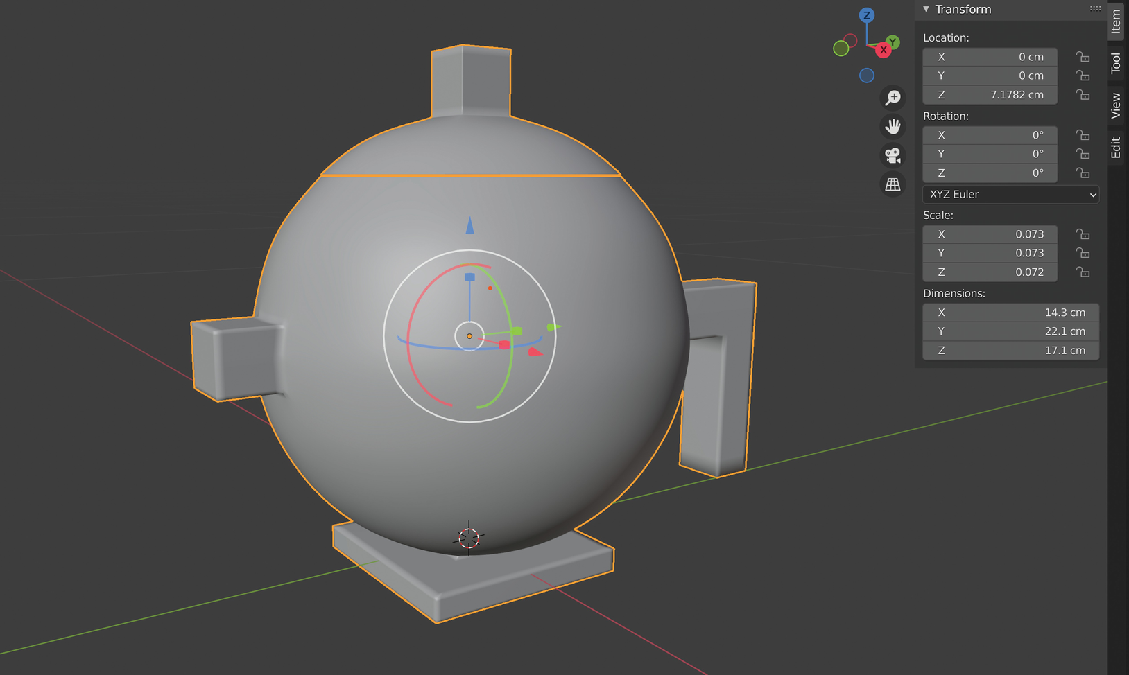
The teapot in solid shading in the 3D viewport
Since we’ve learned about the mesh modeling in Edit mode in this exercise, we will investigate other techniques by rotating a profile with the screw modifier.
Exercise 2: Creating a Glass
Now let’s make a glass; several techniques and modeling possibilities exist.
Since we started from a volume in the first exercise, this time we will begin from a single vertex and extrude a profile and apply the Screw modifier. This method allows us to practice Blender’s essential subobject modeling techniques.
The final result is in the Glass.blend file that accompanies the book.
Follow along with Exercise 2 step-by-step.
Setting the File
Also, in this second exercise, we start by setting up the file to model our objects easily.
- 1.
Repeat steps 1, 2, and 3 of this chapter’s Exercise 1.
Save the file as Glass.blend on the local computer’s drive from the main menu and select File ➤ Save ➤ Save Blender File or press Ctrl+S.
If you don’t want to repeat these steps every time you can save a custom startup file from the main menu and select File ➤ Defaults ➤ Save Startup File, as shown in Figure 2-61.
This way, when you create a new file, it will have the settings you have given it now.

Creating a customized startup file
- 2.
Prepare the scene by selecting the light and the camera, and pressing M. In the window that appears, click New Collection and create another collection called scene. In this way, you have a layer containing the light and the camera, as shown in Figure 2-62.
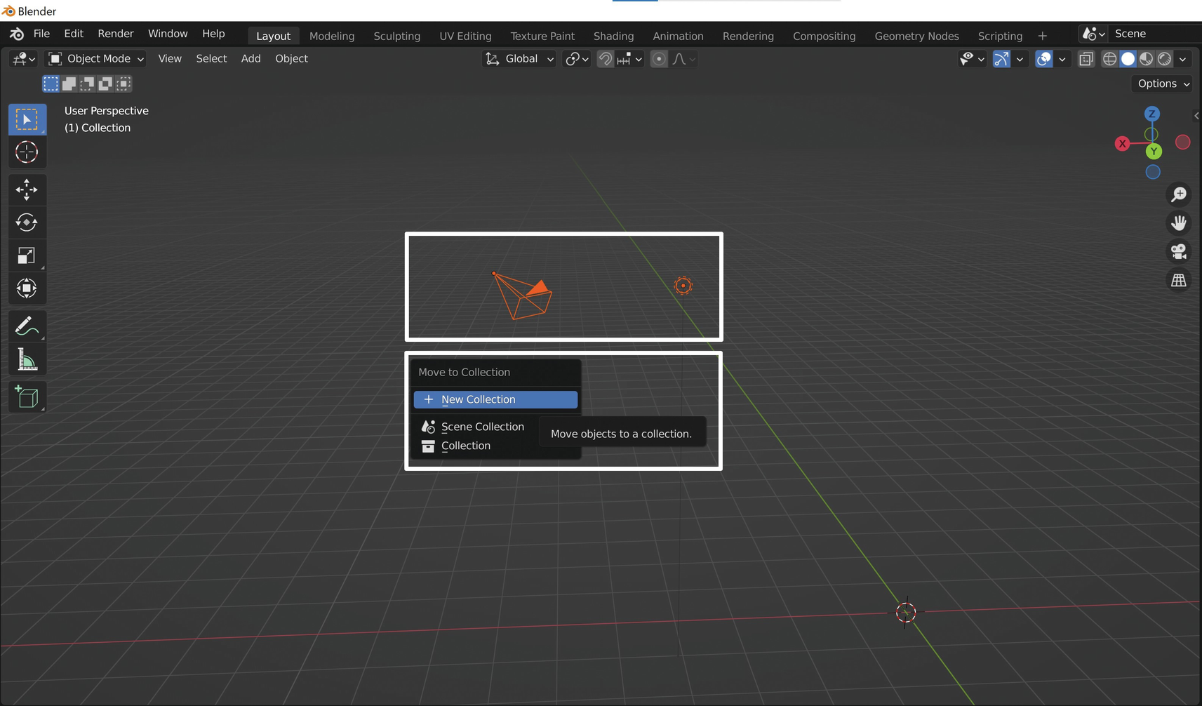
Moving the light and camera in a new collection
- 3.
In the Outliner Editor, click the eye to the right of the scene collection and hide the objects it contains in the 3D view.
Preparing the Basic Object
Now let’s create a reference object to give accurate measurements to our glass. Then we import an image to help us model its profile.
- 1.
Go to the Front Orthographic View by pressing 1 on the Numpad. Then, create a plane by using the Add menu item or by pressing Shift+A ➤ Mesh ➤ Plane, as shown in Figure 2-63.

Creating a plane
- 2.
In the Outliner Editor, when we click the eye to the right of the Scene collection, we can hide or show the objects it contains in the 3D view by toggling the eye symbol on and off, as shown in Figure 2-64.

Controlling the object’s visualization with the collection
- 3.
Select the plane and go to Edit mode by pressing Tab. Select the four vertices if they are not yet selected. Then merge them by clicking M and choosing At center, as shown in Figure 2-65.
This way, the four vertices will join in the center, and there will be only one left.

Merging four vertices into one
- 4.
Select the vertex, select the Plane object in the Outliner, and rename it Glass by double-clicking the Plane name, typing the new name, and pressing Enter to apply it.
- 5.
Go to Edit mode, press B for Border Selection, and drag the left button, selecting the vertex. Then click E ➤ Z ➤ 20 and get a 20-centimeter vertical edge, as shown in Figure 2-66.

Creating the edge for reference
- 6.
Clicking B again selects both vertices, and clicking E ➤ X ➤ 20 creates a 20 by 20-centimeter plane that serves as a reference for your model’s height. The glass is 20 centimeters high.
- 7.
Now press Tab to return to Object mode, press 1 in the Numpad to go to Front Orthographic View, and drag and drop the image Glass, as shown in Figure 2-67.

Creating the reference plane
- 8.
Then select the reference image, move it with G, and shrink it with S such that the height of the glass from bottom to top will be 20 cm, as Figure 2-68.
Pan and zoom the view with the mouse’s central wheel and use the shortcut Shift when necessary.

Positioning the reference image and giving the actual size to the glass
We also could have followed much quicker processes. For example, we could have directly created a plane 20 by 20 centimeters and positioned it frontally in the Front Horthographic View. Nevertheless, the procedure we have chosen, surely more complex, has introduced some essential concepts of the Blender Edit mode.
Creating the Profile and Screwing It
- 1.
Make sure that you still have Glass selected and go to Edit mode. Keep only the bottom vertex, and delete the other three by clicking X and choosing Vertices from the drop-down menu.
- 2.
From the Front Ortho view, move the vertex to the right and select and click E several times to extrude it following the shape of the glass until you get a profile like the one in Figure 2-69.

The profile of the glass to screw
- 3.
In the Properties Editor’s Modifier Properties window, apply the Screw and Subdivision Surface modifiers. Then for the subsurf modifier, change both the Render and Viewport values to 2 or also 3; finally, in this way, you will get the shape of the glass shown in Figure 2-70.

The final glass shape
- 4.
Now apply the Screw modifier first and then Subdivision Surface by clicking the Apply buttons in the Modifiers Properties panel of the Properties editor.
- 5.
Finally, press 1 to enter Vertex mode, select the loop cuts at the bottom of the glass by pressigning Alt, left-click a loop edge, and press F. This creates a face that closes the bottom of the glass.
- 6.
Repeat for the other loop that remains open at the base.
We have started to practice the theoretical information studied until now with these first exercises, and we’ve set a solid foundation for our future work with virtual modeling.
Summary
In this chapter, we learned about the main objects and the fundamental 3D modeling techniques of Blender 3.0. We first studied the modeling objects such as Mesh, Curve, Metaball, etc. Then we analyzed the leading modeling systems: object editing, subobject editing, sculpting, and modifiers. This chapter also showed us the essential techniques of 3D modeling.
In the next chapter, we will see how to create spaces and deal with architectural modeling.