Chapter 5

Video compression and MPEG

5.1 Introduction to compression

Compression allows the same (or nearly the same) information to be represented by a smaller quantity or rate of data. There are several reasons why compression techniques are popular:

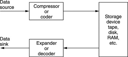
Compression is summarized in Figure 5.1. It will be seen in (a) that the data rate is reduced at source by the compressor. The compressed data are then passed through a communication channel and returned to the original rate by the expander. The ratio between the source data rate and the channel data rate is called the compression factor. The term coding gain is also used. Sometimes a compressor and expander in series are referred to as a compander. The compressor may equally well be referred to as a coder and the expander a decoder in which case the tandem pair may be called a codec.

Figure 5.1 In (a) a compression system consists of compressor or coder, a transmission channel and a matching expander or decoder. The combination of coder and decoder is known as a codec. (b) MPEG is asymmetrical since the encoder is much more complex than the decoder.

Where the encoder is more complex than the decoder the system is said to be asymmetrical as in Figure 5.1(b). The encoder needs to be algorithmic or adaptive whereas the decoder is ‘dumb’ and carries out fixed actions. This is advantageous in applications such as broadcasting where the number of expensive complex encoders is small but the number of simple inexpensive decoders is large. In point-to-point applications the advantage of asymmetrical coding is not so great.

Although there are many different coding techniques, all of them fall into one or other of these categories. In lossless coding, the data from the expander are identical bit-for-bit with the original source data. The so-called ‘stacker’ programs which increase the apparent capacity of disk drives in personal computers use lossless codecs. Clearly, with computer programs the corruption of a single bit can be catastrophic. Lossless coding is generally restricted to compression factors of around 2:1.

In lossy coding data from the expander are not identical bit-for-bit with the source data and as a result comparing the input with the output is bound to reveal differences. Lossy codecs are not suitable for computer data, but are used in MPEG as they allow greater compression factors than lossless codecs. Successful lossy codecs are those in which the errors are arranged so that a human viewer or listener finds them subjectively difficult to detect. Thus lossy codecs must be based on an understanding of psychoacoustic and psychovisual perception and are often called perceptive codes.

In perceptive coding, the greater the compression factor required, the more accurately must the human senses be modelled. Perceptive coders can be forced to operate at a fixed compression factor. This is convenient for practical transmission applications where a fixed data rate is easier to handle than a variable rate. The result of a fixed compression factor is that the subjective quality can vary with the ‘difficulty’ of the input material. Perceptive codecs should not be concatenated indiscriminately especially if they use different algorithms.

Although the adoption of digital techniques is recent, compression itself is as old as television. Figure 5.2 shows some of the compression techniques used in traditional television systems. One of the oldest techniques is interlace which has been used in analog television from the very beginning as a primitive way of reducing bandwidth. As Chapter 2 showed, interlace is not without its problems, particularly in motion rendering. MPEG-2 supports interlace simply because legacy interlaced signals exist and there is a requirement to compress them.

Figure 5.2 Compression is as old as television. (a) Interlace is a primitive way of having the bandwidth. (b) Colour difference working invisibly reduces colour resolution. (c) Composite video transmits colour in the same bandwidth as monochrome.

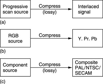
The generation of colour difference signals from RGB in video represents an application of perceptive coding. The human visual system (HVS) sees no change in quality although the bandwidth of the colour difference signals is reduced. This is because human perception of detail in colour changes is much less than in brightness changes. This approach is sensibly retained in MPEG.

Composite video systems such as PAL, NTSC and SECAM are all analog compression schemes which embed a subcarrier in the luminance signal so that colour pictures are available in the same bandwidth as monochrome. In comparison with a progressive scan RGB picture, interlaced composite video has a compression factor of 6:1.

In many respects MPEG-2 is a modern digital equivalent of analog composite video as it has most of the same attributes. For example, the eight-field sequence of a PAL subcarrier which makes editing diffficult has its equivalent in the GOP (group of pictures) of MPEG.1

In a PCM digital system the bit rate is the product of the sampling rate and the number of bits in each sample and this is generally constant. Nevertheless the information rate of a real signal varies. In all real signals, part of the signal is obvious from what has gone before or what may come later and a suitable receiver can predict that part so that only the true information actually has to be sent. If the characteristics of a predicting receiver are known, the transmitter can omit parts of the message in the knowledge that the receiver has the ability to recreate it. Thus all encoders must contain a model of the decoder.

The difference between the information rate and the overall bit rate is known as the redundancy. Compression systems are designed to eliminate as much of that redundancy as practicable or perhaps affordable. One way in which this can be done is to exploit statistical predictability in signals. The information content or entropy of a sample is a function of how different it is from the predicted value. Most signals have some degree of predictability.

At the opposite extreme a signal such as noise is completely unpredictable and as a result all codecs find noise difficult. There are two consequences of this characteristic. First, a codec which is designed using the statistics of real material should not be tested with random noise because it is not a representative test. Second, a codec which performs well with clean source material may perform badly with source material containing superimposed noise. Most practical compression units require some form of preprocessing before the compression stage proper and appropriate noise reduction should be incorporated into the preprocessing if noisy signals are anticipated. It will also be necessary to restrict the degree of compression applied to noisy signals.

All real signals fall part-way between the extremes of total predictability and total unpredictability or noisiness. If the bandwidth (set by the sampling rate) and the dynamic range (set by the wordlength) of the transmission system are used to delineate an area, this sets a limit on the information capacity of the system. Figure 5.3(a) shows that most real signals occupy only part of that area. The signal may not contain all frequencies, or it may not have full dynamics at certain frequencies.

Figure 5.3 (a) A perfect coder removes only the redundancy from the input signal and results in subjectively lossless coding. If the remaining entropy is beyond the capacity of the channel some of it must be lost and the codec will then be lossy. An imperfect coder will also be lossy as it fails to keep all entropy. (b) As the compression factor rises, the complexity must also rise to maintain quality. (c) High compression factors also tend to increase latency or delay through the system.

Entropy can be thought of as a measure of the actual area occupied by the signal. This is the area that must be transmitted if there are to be no subjective differences or artifacts in the received signal. The remaining area is called the redundancy because it adds nothing to the information conveyed. Thus an ideal coder could be imagined which miraculously sorts out the entropy from the redundancy and sends only the former. An ideal decoder would then re-create the original impression of the information quite perfectly.

As the ideal is approached, the coder complexity and the latency or delay both rise. Figure 5.3(b) shows how complexity increases with compression factor. Figure 5.3(c) shows how increasing the codec latency can improve the compression factor. Obviously we would have to provide a channel which could accept whatever entropy the coder extracts in order to have transparent quality. As a result, moderate coding gains which only remove redundancy need not cause artifacts and result in systems which are described as subjectively lossless.

If the channel capacity is not sufficient for that, then the coder will have to discard some of the entropy and with it useful information. Larger coding gains which remove some of the entropy must result in artifacts. It will also be seen from Figure 5.3 that an imperfect coder will fail to separate the redundancy and may discard entropy instead, resulting in artifacts at a suboptimal compression factor.

A single variable-rate transmission or recording channel is inconvenient and unpopular with channel providers because it is difficult to police. The requirement can be overcome by combining several compressed channels into one constant rate transmission in a way which flexibly allocates data rate between the channels. Provided the material is unrelated, the probability of all channels reaching peak entropy at once is very small and so those channels which are at one instant passing easy material will free up transmission capacity for those channels which are handling difficult material. This is the principle of statistical multiplexing.

Where the same type of source material is used consistently, e.g. English text, then it is possible to perform a statistical analysis on the frequency with which particular letters are used. Variable-length coding is used in which frequently used letters are allocated short codes and letters which occur infrequently are allocated long codes. This results in a lossless code. The well-known Morse code used for telegraphy is an example of this approach. The letter e is the most frequent in English and is sent with a single dot. An infrequent letter such as z is allocated a long complex pattern. It should be clear that codes of this kind which rely on a prior knowledge of the statistics of the signal are only effective with signals actually having those statistics. If Morse code is used with another language, the transmission becomes significantly less efficient because the statistics are quite different; the letter z, for example, is quite common in Czech.

The Huffman code2 is one which is designed for use with a data source having known statistics and shares the same principles with the Morse code. The probability of the different code values to be transmitted is studied, and the most frequent codes are arranged to be transmitted with short wordlength symbols. As the probability of a code value falls, it will be allocated a longer wordlength. The Huffman code is used in conjunction with a number of compression techniques and is shown in Figure 5.4.

Figure 5.4 The Huffman code achieves compression by allocating short codes to frequent values. To aid deserializing the short codes are not prefixes of longer codes.

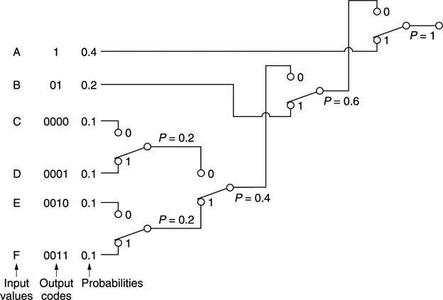
The input or source codes are assembled in order of descending probability. The two lowest probabilities are distinguished by a single code bit and their probabilities are combined. The process of combining probabilities is continued until unity is reached and at each stage a bit is used to distinguish the path. The bit will be a zero for the most probable path and one for the least. The compressed output is obtained by reading the bits which describe which path to take going from right to left.

In the case of computer data, there is no control over the data statistics. Data to be recorded could be instructions, images, tables, text files and so on; each having their own code value distributions. In this case a coder relying on fixed source statistics will be completely inadequate. Instead a system is used which can learn the statistics as it goes along. The Lempel–Ziv–Welch (LZW) lossless codes are in this category. These codes build up a conversion table between frequent long source data strings and short transmitted data codes at both coder and decoder and initially their compression factor is below unity as the contents of the conversion tables are transmitted along with the data. However, once the tables are established, the coding gain more than compensates for the initial loss. In some applications, a continuous analysis of the frequency of code selection is made and if a data string in the table is no longer being used with sufficient frequency it can be deselected and a more common string substituted.

Lossless codes are less common for audio and video coding where perceptive codes are permissible. The perceptive codes often obtain a coding gain by shortening the wordlength of the data representing the signal waveform. This must increase the noise level and the trick is to ensure that the resultant noise is placed at frequencies where human senses are least able to perceive it. As a result although the received signal is measurably different from the source data, it can appear the same to the human listener or viewer at moderate compressions factors. As these codes rely on the characteristics of human sight and hearing, they can only be fully tested subjectively.

The compression factor of such codes can be set at will by choosing the wordlength of the compressed data. Whilst mild compression will be undetectable, with greater compression factors, artifacts become noticeable. Figure 5.3 shows that this is inevitable from entropy considerations.

5.2 What is MPEG?

MPEG is actually an acronym for the Moving Pictures Experts Group which was formed by the ISO (International Standards Organization) to set standards for audio and video compression and transmission. The first compression standard for audio and video was MPEG-13, 4 but this was of limited application and the subsequent MPEG-2 standard was considerably broader in scope and of wider appeal. For example, MPEG-2 supports interlace whereas MPEG-1 did not.

The approach of the ISO to standardization in MPEG is novel because it is not the encoder which is standardized. Figure 5.5(a) shows that instead the way in which a decoder will interpret the bitstream is defined. A decoder which can successfully interpret the bitstream is said to be compliant. Figure 5.5(b) shows that the advantage of standardizing the decoder is that over time, encoding algorithms can improve yet compliant decoders will continue to function with them.

Figure 5.5 (a) MPEG defines the protocol of the bitstream between encoder and decoder. The decoder is defined by implication, the encoder is left very much to the designer. (b) This approach allows future encoders of better performance to remain compatible with existing decoders. (c) This approach also allows an encoder to produce a standard bitstream while its technical operation remains a commercial secret.

Manufacturers can supply encoders using algorithms which are proprietary and their details do not need to be published. A useful result is that there can be competition between different encoder designs which means that better designs will evolve. The user will have greater choice because different levels of cost and complexity can exist in a range of coders yet a compliant decoder will operate with them all.

MPEG is, however, much more than a compression scheme as it also standardizes the protocol and syntax under which it is possible to combine or multiplex audio data with video data to produce a digital equivalent of a television program. Many such programs can be combined in a single multiplex and MPEG defines the way in which such multiplexes can be created and transported. The definitions include the metadata which decoders require to demultiplex correctly and which users will need to locate programs of interest.

As with all video systems there is a requirement for synchronizing or genlocking and this is particularly complex when a multiplex is assembled from many signals which are not necessarily synchronized to one another.

The applications of audio and video compression are limitless and the ISO has done well to provide standards which are appropriate to the wide range of possible compression products.

MPEG-2 embraces video pictures from the tiny screen of a videophone to the high-definition images needed for electronic cinema. Audio coding stretches from speech-grade mono to multichannel surround sound.

Figure 5.6 shows the use of a codec with a recorder. The playing time of the medium is extended in proportion to the compression factor. In the case of tapes, the access time is improved because the length of tape needed for a given recording is reduced and so it can be rewound more quickly.

Figure 5.6 Compression can be used around a recording medium. The storage capacity may be increased or the access time reduced according to the application.

In the case of DVD (digital video disk, aka digital versatile disk) the challenge was to store an entire movie on one 12 cm disk. The storage density available with today’s optical disk technology is such that recording of conventional uncompressed video would be out of the question.

In communications, the cost of data links is often roughly proportional to the data rate and so there is simple economic pressure to use a high compression factor. However, it should be borne in mind that implementing the codec also has a cost which rises with compression factor and so a degree of compromise will be inevitable.

In the case of video-on-demand, technology exists to convey full bandwidth video to the home, but to do so for a single individual at the moment would be prohibitively expensive. Without compression, HDTV (high-definition television) requires too much bandwidth. With compression, HDTV can be transmitted to the home in a similar bandwidth to an existing analog SDTV channel. Compression does not make video-on-demand or HDTV possible, it makes them economically viable.

In workstations designed for the editing of audio and/or video, the source material is stored on hard disks for rapid access. Whilst top-grade systems may function without compression, many systems use compression to offset the high cost of disk storage. When a workstation is used for off-line editing, a high compression factor can be used and artifacts will be visible in the picture.

This is of no consequence as the picture is only seen by the editor who uses it to make an EDL (edit decision list) which is no more than a list of actions and the timecodes at which they occur. The original uncompressed material is then conformed to the EDL to obtain a high-quality edited work. When on-line editing is being performed, the output of the workstation is the finished product and clearly a lower compression factor will have to be used.

Perhaps it is in broadcasting where the use of compression will have its greatest impact. There is only one electromagnetic spectrum and pressure from other services such as cellular telephones makes efficient use of bandwidth mandatory. Analog television broadcasting is an old technology and makes very inefficient use of bandwidth. Its replacement by a compressed digital transmission will be inevitable for the practical reason that the bandwidth is needed elsewhere.

Fortunately in broadcasting there is a mass market for decoders and these can be implemented as low-cost integrated circuits. Fewer encoders are needed and so it is less important if these are expensive. Whilst the cost of digital storage goes down year on year, the cost of electromagnetic spectrum goes up. Consequently in the future the pressure to use compression in recording will ease or even cease whereas the pressure to use it in radio communications will increase.

5.3 Spatial and temporal redundancy in MPEG

Video signals exist in four dimensions: these are the attributes of the sample, the horizontal and vertical spatial axes and the time axis. Compression can be applied in any or all of those four dimensions. MPEG-2 assumes an eight-bit colour difference signal as the input, requiring rounding if the source is ten-bit. The sampling rate of the colour signals is less than that of the luminance. This is done by downsampling the colour samples horizontally and generally vertically as well. Essentially an MPEG-2 system has three parallel simultaneous channels, one for luminance and two for colour difference, which after coding are multiplexed into a single bitstream.

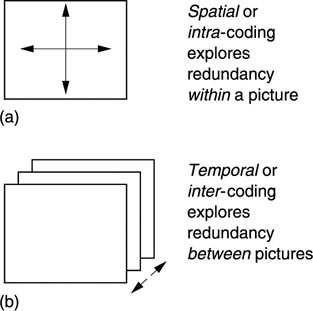
Figure 5.7(a) shows that when individual pictures are compressed without reference to any other pictures, the time axis does not enter the process which is therefore described as intra-coded (intra = within) compression. The term spatial coding will also be found. It is an advantage of intra-coded video that there is no restriction to the editing which can be carried out on the picture sequence. As a result compressed VTRs such as Digital Betacam, DVC and D-9 use spatial coding. Cut editing may take place on the compressed data directly if necessary. As spatial coding treats each picture independently, it can employ certain techniques developed for the compression of still pictures.

Figure 5.7 (a) Spatial or intra-coding works on individual images. (b) Temporal or inter-coding works on successive images.

The ISO JPEG (Joint Photographic Experts Group) compression standards5, 6 are in this category. Where a succession of JPEG coded images are used for television, the term ‘Motion JPEG’ will be found.

Greater compression factors can be obtained by taking account of the redundancy from one picture to the next. This involves the time axis, as Figure 5.7(b) shows, and the process is known as inter-coded (inter = between) or temporal compression.

Temporal coding allows a higher compression factor, but has the disadvantage that an individual picture may exist only in terms of the differences from a previous picture. Clearly, editing must be undertaken with caution and arbitrary cuts simply cannot be performed on the MPEG bitstream. If a previous picture is removed by an edit, the difference data will then be insufficient to re-create the current picture.

Intra-coding works in three dimensions on the horizontal and vertical spatial axes and on the sample values. Analysis of typical television pictures reveals that whilst there is a high spatial frequency content due to detailed areas of the picture, there is a relatively small amount of energy at such frequencies. Often pictures contain sizable areas in which the same or similar pixel values exist. This gives rise to low spatial frequencies. The average brightness of the picture results in a substantial zero frequency component. Simply omitting the high-frequency components is unacceptable as this causes an obvious softening of the picture.

A coding gain can be obtained by taking advantage of the fact that the amplitude of the spatial components falls with frequency. It is further possible to take advantage of the eye’s reduced sensitivity to noise in high spatial frequencies. If the spatial frequency spectrum is divided into frequency bands the high-frequency bands can be described by fewer bits not only because their amplitudes are smaller but also because more noise can be tolerated. The discrete cosine transform introduced in Chapter 2 is used in MPEG to allows two-dimensional pictures to be described in the frequency domain.

Inter-coding takes further advantage of the similarities between successive pictures in real material. Instead of sending information for each picture separately, inter-coders will send the difference between the previous picture and the current picture in a form of differential coding. Figure 5.8 shows the principle. A picture store is required at the coder to allow comparison to be made between successive pictures and a similar store is required at the decoder to make the previous picture available. The difference data may be treated as a picture itself and subjected to some form of transform-based spatial compression.

Figure 5.8 An inter-coded system (a) uses a delay to calculate the pixel differences between successive pictures. To prevent error propagation, intra-coded pictures (b) may be used periodically.

The simple system of Figure 5.8(a) is of limited use as in the case of a transmission error, every subsequent picture would be affected. Channel switching in a television set would also be impossible. In practical systems a modification is required. The approach used in MPEG is that periodically some absolute picture data are transmitted in place of difference data.

Figure 5.8(b) shows that absolute picture data, known as I or intra pictures are interleaved with pictures which are created using difference data, known as P or predicted pictures. The I pictures require a large amount of data, whereas the P pictures require less data. As a result the instantaneous data rate varies dramatically and buffering has to be used to allow a constant transmission rate.

The I picture and all the P pictures prior to the next I picture are called a group of pictures (GOP). For a high compression factor, a large number of P pictures should be present between I pictures, making a long GOP. However, a long GOP delays recovery from a transmission error. The compressed bitstream can only be edited at I pictures as shown.

In the case of moving objects, although their appearance may not change greatly from picture to picture, the data representing them on a fixed sampling grid will change and so large differences will be generated between successive pictures. It is a great advantage if the effect of motion can be removed from difference data so that they only reflect the changes in appearance of a moving object since a much greater coding gain can then be obtained. This is the objective of motion compensation introduced in section 4.5.

It will be clear that the data values representing a moving object change with respect to the time axis. However, looking along the optic flow axis the appearance of an object only changes if it deforms, moves into shadow or rotates. For simple translational motions the data representing an object are highly redundant with respect to the optic flow axis. Thus if the optic flow axis can be located, coding gain can be obtained in the presence of motion.

A motion-compensated coder works as follows. An I picture is sent, but is also locally stored so that it can be compared with the next input picture to find motion vectors for various areas of the picture. The I picture is then shifted according to these vectors to cancel inter-picture motion. The resultant predicted picture is compared with the actual picture to produce a prediction error also called a residual. The prediction error is transmitted with the motion vectors. At the receiver the original I picture is also held in a memory. It is shifted according to the transmitted motion vectors to create the predicted picture and then the prediction error is added to it to re-create the original. When a picture is encoded in this way MPEG calls it a P picture.

Figure 5.9(a) shows that spatial redundancy is redundancy within a single image, for example repeated pixel values in a large area of blue sky. Temporal redundancy (b) exists between successive images.

Figure 5.9 (a) Spatial or intra-coding works on individual images. (b) Temporal or inter-coding works on successive images. (c) In MPEG inter-coding is used to create difference images. These are then compressed spatially.

Where temporal compression is used, the current picture is not sent in its entirety; instead the difference between the current picture and the previous picture is sent. The decoder already has the previous picture, and so it can add the difference to make the current picture. A difference picture is created by subtracting every pixel in one picture from the corresponding pixel in another pixel. This is trivially easy in a progressively scanned system, but MPEG-2 has had to develop greater complexity so that this can also be done with interlaced pictures. The handling of interlace in MPEG will be detailed later.

A difference picture is an image of a kind, although not a viewable one, and so should contain some kind of spatial redundancy. Figure 5.9(c) shows that MPEG-2 takes advantage of both forms of redundancy. Picture differences are spatially compressed prior to transmission. At the decoder the spatial compression is decoded to re-create the difference picture, then this difference picture is added to the previous picture to complete the decoding process.

Whenever objects move they will be in a different place in successive pictures. This will result in large amounts of difference data. MPEG-2 overcomes the problem using motion compensation. The encoder contains a motion estimator which measures the direction and distance of motion between pictures and outputs these as vectors which are sent to the decoder. When the decoder receives the vectors it uses them to shift data in a previous picture to more closely resemble the current picture. Effectively the vectors are describing the optic flow axis of some moving screen area, along which axis the image is highly redundant. Vectors are bipolar codes which determine the amount of horizontal and vertical shift required.

In real images, moving objects do not necessarily maintain their appearance as they move. For example, objects may turn, move into shade or light, or move behind other objects. Consequently motion compensation can never be ideal and it is still necessary to send a picture difference to make up for any shortcomings in the motion compensation.

Figure 5.10 shows how this works. In addition to the motion encoding system, the coder also contains a motion decoder. When the encoder outputs motion vectors, it also uses them locally in the same way that a real decoder will, and is able to produce a predicted picture based solely on the previous picture shifted by motion vectors. This is then subtracted from the actual current picture to produce a prediction error or residual which is an image of a kind that can be spatially compressed.

Figure 5.10 A motion-compensated compression system. The coder calculates motion vectors which are transmitted as well as being used locally to create a predicted picture. The difference between the predicted picture and the actual picture is transmitted as a prediction error.

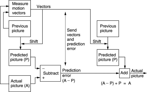
The decoder takes the previous picture, shifts it with the vectors to re-create the predicted picture and then decodes and adds the prediction error to produce the actual picture. Picture data sent as vectors plus prediction error are said to be P coded.

The concept of sending a prediction error is a useful approach because it allows both the motion estimation and compensation to be imperfect.

A good motion-compensation system will send just the right amount of vector data. With insufficient vector data, the prediction error will be large, but transmission of excess vector data will also cause the the bit rate to rise. There will be an optimum balance which minimizes the sum of the prediction error data and the vector data.

In MPEG-2 the balance is obtained by dividing the screen into areas called macroblocks which are 16 luminance pixels square. Each macroblock is steered by a vector. The location of the boundaries of a macroblock are fixed and so the vector does not move the macroblock. Instead the vector tells the decoder where to look in another frame to find pixel data to fetch to the macroblock. Figure 5.11(a) shows this concept. The shifting process is generally done by modifying the read address of a RAM using the vector. This can shift by one-pixel steps. MPEG-2 vectors have half-pixel resolution so it is necessary to interpolate between pixels from RAM to obtain half-pixel shifted values.

Figure 5.11 (a) In motion compensation, pixel data are brought to a fixed macroblock in the target picture from a variety of places in another picture. (b) Where only part of a macroblock is moving, motion compensation is non-ideal. The motion can be coded (c), causing a prediction error in the background, or the background can be coded (d) causing a prediction error in the moving object.

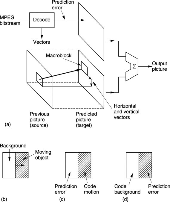
Real moving objects will not coincide with macroblocks and so the motion compensation will not be ideal but the prediction error makes up for any shortcomings. Figure 5.11(b) shows the case where the boundary of a moving object bisects a macroblock. If the system measures the moving part of the macroblock and sends a vector, the decoder will shift the entire block making the stationary part wrong. If no vector is sent, the moving part will be wrong. Both approaches are legal in MPEG-2 because the prediction error sorts out the incorrect values. An intelligent coder might try both approaches to see which required the least prediction error data.

The prediction error concept also allows the use of simple but inaccurate motion estimators in low-cost systems. The greater prediction error data is handled using a higher bit rate. On the other hand, if a precision motion estimator is available, a very high compression factor may be achieved because the prediction error data are minimized. MPEG-2 does not specify how motion is to be measured; it simply defines how a decoder will interpret the vectors. Encoder designers are free to use any motion-estimation system provided that the right vector protocol is created.

Figure 5.12(a) shows that a macroblock contains both luminance and colour difference data at different resolutions. Most of the MPEG-2 Profiles use a 4:2:0 structure which means that the colour is downsampled by a factor of two in both axes. Thus in a 16 × 16 pixel block, there are only 8 × 8 colour difference sampling sites. MPEG-2 is based upon the 8 × 8 DCT (see section 2.24) and so the 16 × 16 block is the screen area which contains an 8 × 8 colour difference sampling block. Thus in 4:2:0 in each macroblock there are four luminance DCT blocks, one R–Y DCT block and one B–Y DCT block, all steered by the same vector.

Figure 5.12 The structure of a macroblock. (A macroblock is the screen area steered by one vector.) (a) In 4:2:0, there are two chroma DCT blocks per macroblock whereas in 4:2:2 (b) there are four. 4:2:2 needs 33% more data than 4:2:0.

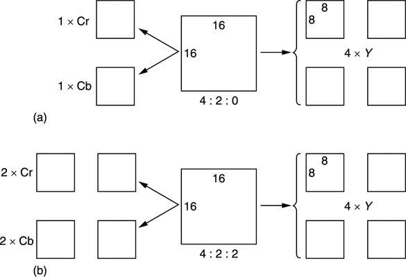
In the 4:2:2 Profile of MPEG-2, shown in Figure 5.12(b), the chroma is not downsampled vertically, and so there is twice as much chroma data in each macroblock which is otherwise substantially the same.

5.4 I and P coding

Predictive (P) coding cannot be used indefinitely, as it is prone to error propagation. A further problem is that it becomes impossible to decode the transmission if reception begins part-way through. In real video signals, cuts or edits can be present across which there is little redundancy and which make motion estimators throw up their hands.

In the absence of redundancy over a cut, there is nothing to be done but to send the new picture information in absolute form. This is called I coding where I is an abbreviation of intra coding. As I coding needs no previous picture for decoding, then decoding can begin at I coded information.

MPEG-2 is effectively a toolkit and there is no compulsion to use all the tools available. Thus an encoder may choose whether to use I or P coding, either once and for all or dynamically on a macroblock-by-macroblock basis.

For practical reasons, an entire frame may be encoded as I macroblocks periodically. This creates a re-entry point where the bitstream might be edited or where decoding could begin.

Figure 5.13 shows a typical application of the Simple Profile of MPEG-2. Periodically an I picture is created. Between I pictures are P pictures which are based on the picture before. These P pictures predominantly contain macroblocks having vectors and prediction errors. However, it is perfectly legal for P pictures to contain I macroblocks. This might be useful where, for example, a camera pan introduces new material at the edge of the screen which cannot be created from an earlier picture.

Figure 5.13 A Simple Profile MPEG-2 signal may contain periodic I pictures with a number of P pictures between.

Note that although what is sent is called a P picture, it is not a picture at all. It is a set of instructions to convert the previous picture into the current picture. If the previous picture is lost, decoding is impossible. An I picture together with all the pictures before the next I picture form a group of pictures (GOP).

5.5 Bidirectional coding

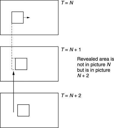
Motion-compensated predictive coding is a useful compression technique, but it does have the drawback that it can only take data from a previous picture. Where moving objects reveal a background this is completely unknown in previous pictures and forward prediction fails. However, more of the background is visible in later pictures. Figure 5.14 shows the concept. In the centre of the diagram, a moving object has revealed some background. The previous picture can contribute nothing, whereas the next picture contains all that is required.

Figure 5.14 In bidirectional coding the revealed background can be efficiently coded by bringing data back from a future picture.

Bidirectional coding is shown in Figure 5.15. A bidirectional or B macroblock can be created using a combination of motion compensation and the addition of a prediction error. This can be done by forward prediction from a previous picture or backward prediction from a subsequent picture. It is also possible to use an average of both forward and backward prediction. On noisy material this may result in some reduction in bit rate. The technique is also a useful way of portraying a dissolve.

Figure 5.15 In bidirectional coding, a number of B pictures can be inserted between periodic forward predicted pictures. See text.

The averaging process in MPEG-2 is a simple linear interpolation which works well when only one B picture exists between the reference pictures before and after. A larger number of B pictures would require weighted interpolation but MPEG-2 does not support this.

Typically two B pictures are inserted between P pictures or between I and P pictures. As can be seen, B pictures are never predicted from one another, only from I or P pictures. A typical GOP for broadcasting purposes might have the structure IBBPBBPBBPBB. Note that the last B pictures in the GOP require the I picture in the next GOP for decoding and so the GOPs are not truly independent. Independence can be obtained by creating a closed GOP which may contain B pictures but which ends with a P picture. It is also legal to have a B picture in which every macroblock is forward predicted, needing no future picture for decoding.

Bidirectional coding is very powerful. Figure 5.16 is a constant quality curve showing how the bit rate changes with the type of coding. On the left, only I or spatial coding is used, whereas on the right an IBBP structure is used. This means that there are two bidirectionally coded pictures in between a spatially coded picture (I) and a forward predicted picture (P). Note how for the same quality the system which only uses spatial coding needs two and a half times the bit rate that the bidirectionally coded system needs.

Figure 5.16 Bidirectional coding is very powerful as it allows the same quality with only 40 per cent of the bit rate of intra-coding. However, the encoding and decoding delays must increase. Coding over a longer time span is more efficient but editing is more difficult.

Clearly information in the future has yet to be transmitted and so is not normally available to the decoder. MPEG-2 gets around the problem by sending pictures in the wrong order. Picture reordering requires delay in the encoder and a delay in the decoder to put the order right again. Thus the overall codec delay must rise when bidirectional coding is used. This is quite consistent with Figure 5.3 which showed that as the compression factor rises the latency must also rise.

Figure 5.17 shows that although the original picture sequence is IBBPBBPBBIBB …, this is transmitted as IPBBPBBIBB … so that the future picture is already in the decoder before bidirectional decoding begins. Note that the I picture of the next GOP is actually sent before the last B pictures of the current GOP.

Figure 5.17 Comparison of pictures before and after compression showing sequence change and varying amount of data needed by each picture type. I, P, B pictures use unequal amounts of data.

Figure 5.17 also shows that the amount of data required by each picture is dramatically different. I pictures have only spatial redundancy and so need a lot of data to describe them. P pictures need fewer data because they are created by shifting the I picture with vectors and then adding a prediction error picture. B pictures need the least data of all because they can be created from I or P.

With pictures requiring a variable length of time to transmit, arriving in the wrong order, the decoder needs some help. This takes the form of picture-type flags and time stamps.

Figure 5.18 shows a variety of GOP structures. The simplest is the III … sequence in which every picture is intra-coded. Pictures can be fully decoded without reference to any other pictures and so editing is straightforward. However, this approach requires about two and one half times the bit rate of a full bidirectional system. Bidirectional coding is most useful for final delivery of post-produced material either by broadcast or on prerecorded media as there is then no editing requirement. As a compromise the IBIB structure can be used which has some of the bit rate advantage of bidirectional coding but without too much latency. It is possible to edit an IBIB stream by performing some processing. If it is required to remove the video following a B picture, that B picture could not be decoded because it needs I pictures either side of it for bidirectional decoding. The solution is to decode the B picture first, and then reencode it with forward prediction only from the previous I picture. The subsequent I picture can then be replaced by an edit process. Some quality loss is inevitable in this process but this is acceptable in applications such as ENG and industrial video.

Figure 5.18 Various possible GOP structures used with MPEG. See text for details.

5.6 Spatial compression

Spatial compression in MPEG-2 is used in I pictures on actual picture data and in P and B pictures on prediction error data. MPEG-2 uses the discrete cosine transform described in section 2.24. The DCT works on blocks and in MPEG-2 these are 8 x 8 pixels. The macroblocks of the motion-compensation structure are designed so they can be broken down into 8 x 8 DCT blocks. In a 4:2:0 macroblock there will be six DCT blocks whereas in a 4:2:2 macroblock there will be eight.

Figure 5.19 shows the table of basis functions or wave table for an 8 x 8 DCT. Adding these two-dimensional waveforms together in different proportions will give any original 8 x 8 pixel block. The coefficients of the DCT simply control the proportion of each wave which is added in the inverse transform. The top-left wave has no modulation at all because it conveys the DC component of the block. This coefficient will be a unipolar (positive only) value in the case of luminance and will typically be the largest value in the block as the spectrum of typical video signals is dominated by the DC component.

Figure 5.19 The discrete cosine transform breaks up an image area into discrete frequencies in two dimensions. The lowest frequency can be seen here at the top-left corner. Horizontal frequency increases to the right and vertical frequency increases downwards.

Increasing the DC coefficient adds a constant amount to every pixel. Moving to the right the coefficients represent increasing horizontal spatial frequencies and moving downwards they represent increasing vertical spatial frequencies. The bottom-right coefficient represents the highest diagonal frequencies in the block. All these coefficients are bipolar, where the polarity indicates whether the original spatial waveform at that frequency was inverted.

Figure 5.20 shows a one-dimensional example of an inverse transform. The DC coefficient produces a constant level throughout the pixel block. The remaining waves in the table are AC coefficients. A zero coefficient would result in no modulation, leaving the DC level unchanged. The wave next to the DC component represents the lowest frequency in the transform which is half a cycle per block. A positive coefficient would make the left side of the block brighter and the right side darker whereas a negative coefficient would do the opposite. The magnitude of the coefficient determines the amplitude of the wave which is added. Figure 5.20 also shows that the next wave has a frequency of one cycle per block. i.e. the block is made brighter at both sides and darker in the middle.

Figure 5.20 A one-dimensional inverse transform. See text for details.

Consequently an inverse DCT is no more than a process of mixing various pixel patterns from the wave table where the relative amplitudes and polarity of these patterns are controlled by the coefficients. The original transform is simply a mechanism which finds the coefficient amplitudes from the original pixel block.

The DCT itself achieves no compression at all. Sixty-four pixels are converted to sixty-four coefficients. However, in typical pictures, not all coefficients will have significant values; there will often be a few dominant coefficients. The coefficients representing the higher two-dimensional spatial frequencies will often be zero or of small value in large areas, due to blurring or simply plain undetailed areas before the camera.

Statistically, the further from the top-left corner of the wave table the coefficient is, the smaller will be its magnitude. Coding gain (the technical term for reduction in the number of bits needed) is achieved by transmitting the low-valued coefficients with shorter wordlengths. The zero-valued coefficients need not be transmitted at all. Thus it is not the DCT which compresses the data, it is the subsequent processing. The DCT simply expresses the data in a form which makes the subsequent processing easier.

Higher compression factors require the coefficient wordlength to be further reduced using requantizing. Coefficients are divided by some factor which increases the size of the quantizing step. The smaller number of steps which results permits coding with fewer bits, but, of course, with an increased quantizing error. The coefficients will be multiplied by a reciprocal factor in the decoder to return to the correct magnitude.

Inverse transforming a requantized coefficient means that the frequency it represents is reproduced in the output with the wrong amplitude. The difference between original and reconstructed amplitude is regarded as a noise added to the wanted data. Figure 5.21 shows that the visibility of such noise is far from uniform. The maximum sensitivity is found at DC and falls thereafter. As a result, the top-left coefficient is often treated as a special case and left unchanged. It may warrant more error protection than other coefficients.

Figure 5.21 The sensitivity of the eye to noise is greatest at low frequencies and drops rapidly with increasing frequency. This can be used to mask quantizing noise caused by the compression process.

MPEG-2 takes advantage of the falling sensitivity to noise. Prior to requantizing, each coefficient is divided by a different weighting constant as a function of its frequency. Figure 5.22 shows a typical weighting process. Naturally the decoder must have a corresponding inverse weighting. This weighting process has the effect of reducing the magnitude of high-frequency coefficients disproportionately. Clearly, different weighting will be needed for colour difference data as colour is perceived differently.

Figure 5.22 Weighting is used to make the noise caused by requantizing different at each frequency.

P and B pictures are decoded by adding a prediction error image to a reference image. That reference image will contain weighted noise. One purpose of the prediction error is to cancel that noise to prevent tolerance build-up. If the prediction error were also to contain weighted noise this result would not be obtained. Consequently prediction error coefficients are flat weighted.

When forward prediction fails, such as in the case of new material introduced in a P picture by a pan, P coding would set the vectors to zero and encode the new data entirely as an unweighted prediction error. In this case it is better to encode that material as an I macroblock because then weighting can be used and this will require fewer bits.

Requantizing increases the step size of the coefficients, but the inverse weighting in the decoder results in step sizes which increase with frequency. The larger step size increases the quantizing noise at high frequencies where it is less visible. Effectively the noise floor is shaped to match the sensitivity of the eye. The quantizing table in use at the encoder can be transmitted to the decoder periodically in the bitstream.

Study of the signal statistics gained from extensive analysis of real material is used to measure the probability of a given coefficient having a given value. This probability turns out to be highly non-uniform, suggesting the possibility of a variable-length encoding for the coefficient values. On average, the higher the spatial frequency, the lower the value of a coefficient will be. This means that the value of a coefficient falls as a function of its radius from the DC coefficient.

Typical material often has many coefficients which are zero valued, especially after requantizing. The distribution of these also follows a pattern. The non-zero values tend to be found in the top-left-hand corner of the DCT block, but as the radius increases, not only do the coefficient values fall, but it becomes increasingly likely that these small coefficients will be interspersed with zero-valued coefficients. As the radius increases further it is probable that a region where all coefficients are zero will be entered.

MPEG-2 uses all these attributes of DCT coefficients when encoding a coefficient block. By sending the coefficients in an optimum order, by describing their values with Huffman coding and by using run-length encoding for the zero-valued coefficients it is possible to achieve a significant reduction in coefficient data which remains entirely lossless. Despite the complexity of this process, it does contibute to improved picture quality because for a given bit rate lossless coding of the coefficients must be better than requantizing, which is lossy. Of course, for lower bit rates both will be required.

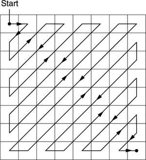
It is an advantage to scan in a sequence where the largest coefficient values are scanned first. Then the next coefficient is more likely to be zero than the previous one. With progressively scanned material, a regular zig-zag scan begins in the top-left corner and ends in the bottom-right corner as shown in Figure 5.23. Zigzag scanning means that significant values are more likely to be transmitted first, followed by the zero values. Instead of coding these zeros, an unique ‘end of block’ (EOB) symbol is transmitted instead.

Figure 5.23 The zig-zag scan for a progressively scanned image.

As the zig-zag scan approaches the last finite coefficient it is increasingly likely that some zero-value coefficients will be scanned. Instead of transmitting the coefficients as zeros, the zero-run-length, i.e. the number of zero valued coefficients in the scan sequence, is encoded into the next non-zero coefficient which is itself variable-length coded. This combination of run-length and variable-length coding is known as RLC/VLC in MPEG-2.

The DC coefficient is handled separately because it is differentially coded and this discussion relates to the AC coefficients. Three items need to be handled for each coefficient: the zero-run-length prior to this coefficient, the wordlength and the coefficient value itself. The wordlength needs to be known by the decoder so that it can correctly parse the bitstream. The wordlength of the coefficient is expressed directly as an integer called the size.

Figure 5.24(a) shows that a two-dimensional run/size table is created. One dimension expresses the zero-run-length; the other the size. A run length of zero is obtained when adjacent coefficients are non-zero, but a code of 0/0 has no meaningful run/size interpretation and so this bit pattern is used for the EOB symbol.

Figure 5.24 Run-length and variable-length coding simultaneously compresses runs of zero-valued coefficients and describes the wordlength of a non-zero coefficient.

In the case where the zero-run-length exceeds 14, a code of 15/0 is used, signifying that there are fifteen zero-valued coefficients. This is then followed by another run/size parameter whose run-length value is added to the previous fifteen.

The run/size parameters contain redundancy because some combinations are more common than others. Figure 5.24(b) shows that each run/size value is converted to a variable-length Huffman codeword for transmission. The Huffman codes are designed so that short codes are never a prefix of long codes so that the decoder can deduce the parsing by testing an increasing number of bits until a match with the look-up table is found. Having parsed and decoded the Huffman run/size code, the decoder then knows what the coefficient wordlength will be and can correctly parse that.

The variable-length coefficient code has to describe a bipolar coefficient, i.e one which can be positive or negative. Figure 5.24(c) shows that for a particular size, the coding scale has a certain gap in it. For example, all values from–7 to + 7 can be sent by a size 3 code, so a size 4 code only has to send the values of –15 to –8 and + 8 to + 15. The coefficient code is sent as a pure binary number whose value ranges from all zeros to all ones where the maximum value is a function of the size. The number range is divided into two, the lower half of the codes specifying negative values and the upper half specifying positive.

In the case of positive numbers, the transmitted binary value is the actual coefficient value, whereas in the case of negative numbers a constant must be subtracted which is a function of the size. In the case of a size 4 code, the constant is 15₁₀. Thus a size 4 parameter of 0111₂ (7₁₀) would be interpreted as 7–15 = 8. A size of 5 has a constant of 31 so a transmitted coded of 01010₂(10₂) would be interpreted as 10–31 = -21.

This technique saves a bit because, for example, 63 values from–31 to + 31 are coded with only 5 bits having only 32 combinations. This is possible because that extra bit is effectively encoded into the run/size parameter.

Figure 5.25 shows the whole spatial coding subsystem. Macroblocks are subdivided into DCT blocks and the DCT is calculated. The resulting coefficients are multiplied by the weighting matrix and then requantized. The coefficients are then reordered by the zig-zag scan so that full advantage can be taken of run-length and variable-length coding. The last non-zero coefficient in the scan is followed by the EOB symbol.

Figure 5.25 A complete spatial coding system which can compress an I picture or the prediction error in P and B pictures. See text for details.

In predictive coding, sometimes the motion-compensated prediction is nearly exact and so the prediction error will be almost zero. This can also happen on still parts of the scene. MPEG-2 takes advantage of this by sending a code to tell the decoder there is no prediction error data for the macroblock concerned.

The success of temporal coding depends on the accuracy of the vectors. Trying to reduce the bit rate by reducing the accuracy of the vectors is false economy as this simply increases the prediction error. Consequently for a given GOP structure it is only in the spatial coding that the overall bit rate is determined. The RLC/VLC coding is lossless and so its contribution to the compression cannot be varied. If the bit rate is too high, the only option is to increase the size of the coefficient-requantizing steps. This has the effect of shortening the wordlength of large coefficients, and rounding small coefficients to zero, so that the bit rate goes down. Clearly, if taken too far the picture quality will also suffer because at some point the noise floor will become visible as some form of artifact.

5.7 A bidirectional coder

MPEG-2 does not specify how an encoder is to be built or what coding decisions it should make. Instead it specifies the protocol of the bitstream at the output. As a result the coder shown in Figure 5.26 is only an example.

Figure 5.26 A bidirectional coder. (a) The essential components. (b) Signal flow when coding an I picture. (c) Signal flow when coding a P picture. (d) Signal flow when bidirectional coding.

Figure 5.26(a) shows the component parts of the coder. At the input is a chain of picture stores which can be bypassed for reordering purposes. This allows a picture to be encoded ahead of its normal timing when bidirectional coding is employed.

At the centre is a dual-motion estimator which can simultaneously measure motion between the input picture an earlier picture and a later picture. These reference pictures are held in frame stores. The vectors from the motion estimator are used locally to shift a picture in a frame store to form a predicted picture. This is subtracted from the input picture to produce a prediction error picture which is then spatially coded.

The bidirectional encoding process will now be described. A GOP begins with an I picture which is intra coded. In Figure 5.26(b) the I picture emerges from the reordering delay. No prediction is possible on an I picture so the motion estimator is inactive. There is no predicted picture and so the prediction error subtractor is set simply to pass the input. The only processing which is active is the forward spatial coder which describes the picture with DCT coefficients. The output of the forward spatial coder is locally decoded and stored in the past picture frame store.

The reason for the spatial encode/decode is that the past picture frame store now contains exactly what the decoder frame store will contain, including the effects of any requantizing errors. When the same picture is used as a reference at both ends of a differential coding system, the errors will cancel out.

Having encoded the I picture, attention turns to the P picture. The input sequence is IBBP, but the transmitted sequence must be IPBB. Figure 5.26(c) shows that the reordering delay is bypassed to select the P picture. This passes to the motion estimator which compares it with the I picture and outputs a vector for each macroblock. The forward predictor uses these vectors to shift the I picture so that it more closely resembles the P picture. The predicted picture is then subtracted from the actual picture to produce a forward prediction error. This is then spatially coded. Thus the P picture is transmitted as a set of vectors and a prediction error image.

The P picture is locally decoded in the right-hand decoder. This takes the forward predicted picture and adds the decoded prediction error to obtain exactly what the decoder will obtain.

Figure 5.26(d) shows that the encoder now contains a I picture in the left store and a P picture in the right store. The reordering delay is reselected so that the first B picture can be input. This passes to the motion estimator where it is compared with both the I and P pictures to produce forward and backward vectors. The forward vectors go to the forward predictor to make a B prediction from the I picture. The backward vectors go to the backward predictor to make a B prediction from the P picture. These predictions are simultaneously subtracted from the actual B picture to produce a forward prediction error and a backward prediction error. These are then spatially encoded. The encoder can then decide which direction of coding resulted in the best prediction; i.e. the smallest prediction error.

Not shown in the interests of clarity is a third signal path which creates a predicted B picture from the average of forward and backward predictions. This is subtracted from the input picture to produce a third prediction error. In some circumstances this prediction error may use fewer data than either forward of backward prediction alone.

As B pictures are never used to create other pictures, the decoder does not locally decode the B picture. After decoding and displaying the B picture the decoder will discard it. At the encoder the I and P pictures remain in their frame stores and the second B picture is input from the reordering delay.

Following the encoding of the second B picture, the encoder must reorder again to encode the second P picture in the GOP. This will be locally decoded and will replace the I picture in the left store. The stores and predictors switch designation because the left store is now a future P picture and the right store is now a past P picture. B pictures between them are encoded as before.

There is still some redundancy in the output of a bidirectional coder and MPEG-2 is remarkably diligent in finding it. In I pictures, the DC coefficient describes the average brightness of an entire DCT block. In real video the DC component of adjacent blocks will be similar much of the time. A saving in bit rate can be obtained by differentially coding the DC coefficient.

In P and B pictures this is not done because these are prediction errors not actual images and the statistics are different. However, P and B pictures send vectors and instead the redundancy in these is explored. In a large moving object, many macroblocks will be moving at the same velocity and their vectors will be the same. Thus differential vector coding will be advantageous.

As has been seen above, differential coding cannot be used indiscriminately as it is prone to error propagation. Periodically absolute DC coefficients and vectors must be sent and the slice is the logical structure which supports this mechanism. In I pictures, the first DC coefficient in a slice is sent in absolute form, whereas the subsequent coefficients are sent differentially. In P or B pictures, the first vector in a slice is sent in absolute form, but the subsequent vectors are differential.

Slices are horizontal picture strips which are one macroblock (16 pixels) high and which proceed from left to right across the screen. The sides of the picture must coincide with the beginning or the end of a slice in MPEG-2, but otherwise the encoder is free to decide how big slices should be and where they begin.

In the case of a central dark building silhouetted against the bright sky, there would be two large changes in the DC coefficients, one at each edge of the building. It may be advantageous to the encoder to break the width of the picture into three slices, one each for the left and right areas of sky and one for the building. In the case of a large moving object, different slices may be used for the object and the background.

Each slice contains its own synchronizing pattern, so following a transmission error, correct decoding can resume at the next slice. Slice size can also be matched to the characteristics of the transmission channel. For example, in an error-free transmission system the use of a large number of slices in a packet simply wastes data capacity on surplus synchronizing patterns. However, in a non-ideal system it might be advantageous to have frequent resynchronizing.

5.8 Handling interlaced pictures

Spatial coding, predictive coding and motion compensation can still be performed using interlaced source material at the cost of considerable complexity. Despite that complexity, MPEG-2 cannot be expected to perform as well with interlaced material.

Figure 5.27 shows that in an incoming interlaced frame there are two fields each of which contain half of the lines in the frame. In MPEG-2 these are known as the top field and the bottom field. In video from a camera, these fields represent the state of the image at two different times. Where there is little image motion, this is unimportant and the fields can be combined obtaining more effective compression. However, in the presence of motion the fields become increasingly decorrelated because of the displacement of moving objects from one field to the next.

Figure 5.27 An interlaced frame consists of top and bottom fields. MPEG-2 can code a frame in the ways shown here.

This characteristic determines that MPEG-2 must be able to handle fields independently or together. This dual approach permeates all aspects of MPEG-2 and affects the definition of pictures, macroblocks, DCT blocks and zig-zag scanning.

Figure 5.27 also shows how MPEG-2 designates interlaced fields. In picture types I, P and B, the two fields can be superimposed to make a frame-picture or the two fields can be coded independently as two field-pictures. As a third possibility, in I pictures only, the bottom field-picture can be predictively coded from the top field-picture to make an IP frame-picture.

A frame-picture is one in which the macroblocks contain lines from both field types over a picture area sixteen scan lines high. Each luminance macroblock contains the usual four DCT blocks but there are two ways in which these can be assembled. Figure 5.28(a) shows how a frame is divided into frame DCT blocks. This is identical to the progressive scan approach in that each DCT block contains eight contiguous picture lines. In 4:2:0, the colour difference signals have been downsampled by a factor of two and shifted. Figure 5.28(a) also shows how one 4:2:0 DCT block contains the chroma data from sixteen lines in two fields.

Figure 5.28 (a) In Frame-DCT, a picture is effectively de-interlaced. (b) In Field-DCT, each DCT block only contains lines from one field, but over twice the screen area. (c) The same DCT content results when field-pictures are assembled into blocks.

Even small amounts of motion in any direction can destroy the correlation between odd and even lines and a frame DCT will result in an excessive number of coefficients. Figure 5.28(b) shows that instead the luminance component of a frame can also be divided into field DCT blocks. In this case one DCT block contains odd lines and the other contains even lines. In this mode the chroma still produces one DCT block from both fields as in Figure 5.28(a).

When an input frame is designated as two field-pictures, the macroblocks come from a screen area which is thirty two lines high. Figure 5.28(c) shows that the DCT blocks contain the same data as if the input frame had been designated a frame-picture but with field DCT. Consequently it is only frame-pictures which have the option of field or frame DCT. These may be selected by the encoder on a macroblock-by-macroblock basis and, of course, the resultant bitstream must specify what has been done.

In a frame which contains a small moving area, it may be advantageous to encode as a frame-picture with frame DCT except in the moving area where field DCT is used. This approach may result in fewer bits than coding as two field-pictures.

In a field-picture and in a frame-picture using field DCT, a DCT block contains lines from one field type only and this must have come from a screen area sixteen scan lines high, whereas in progressive scan and frame DCT the area is only eight scan lines high. A given vertical spatial frequency in the image is sampled at points twice as far apart which is interpreted by the field DCT as a doubled spatial frequency, whereas there is no change in the horizontal spectrum.

Following the DCT calculation, the coefficient distribution will be different in field-pictures and field DCT frame-pictures. In these cases, the probability of coefficients is not a constant function of radius from the DC coefficient as it is in progressive scan, but is elliptical where the ellipse is twice as high as it is wide.

Using the standard 45° zig-zag scan with this different coefficient distribution would not have the required effect of putting all the significant coefficients at the beginning of the scan. To achieve this requires a different zig-zag scan, which is shown in Figure 5.29. This scan, sometimes known as the Yeltsin walk, attempts to match the elliptical probability of interlaced coefficients with a scan slanted at 67.5° to the vertical. This is clearly suboptimal, and is one of the reasons why MPEG-2 does not work so well with interlaced video.

Figure 5.29 The zig-zag scan for an interlaced image has to favour vertical frequencies twice as much as horizontal.

Motion estimation is more difficult in an interlaced system. Vertical detail can result in differences between fields and this reduces the quality of the match. Fields are vertically subsampled without filtering and so contain alias products. This aliasing will mean that the vertical waveform representing a moving object will not be the same in successive pictures and this will also reduce the quality of the match.

Even when the correct vector has been found, the match may be poor so the estimator fails to recognize it. If it is recognized, a poor match means that the quality of the prediction in P and B pictures will be poor and so a large prediction error or residual has to be transmitted. In an attempt to reduce the residual, MPEG-2 allows field-pictures to use motion-compensated prediction from either the adjacent field or from the same field type in another frame. In this case the encoder will use the better match. This technique can also be used in areas of frame-pictures which use field DCT.

The motion compensation of MPEG-2 has half-pixel resolution and this is inherently compatible with an interlace because an interpolator must be present to handle the half-pixel shifts. Figure 5.30(a) shows that in an interlaced system, each field contains half of the frame lines and so interpolating half-way between lines of one field type will actually create values lying on the sampling structure of the other field type. Thus it is equally possible for a predictive system to decode a given field type based on pixel data from the other field type or of the same type.

Figure 5.30 (a) Each field contains half of the frame lines and so interpolation is needed to create values lying on the sampling structure of the other field type. (b) Prediction can use data from the previous field or the one before that.

If when using predictive coding from the other field type the vertical motion vector contains a half-pixel component, then no interpolation is needed because the act of transferring pixels from one field to another results in such a shift.

Figure 5.30(b) shows that a macroblock in a given P field-picture can be encoded using a vector which shifts data from the previous field or from the field before that, irrespective of which frames these fields occupy. As noted above, field-picture macroblocks come from an area of screen thirty-two lines high and this means that the vector density is halved resulting in larger prediction errors at the boundaries of moving objects.

As an option, field-pictures can restore the vector density by using 16 x 8 motion compensation where separate vectors are used for the top and bottom halves of the macroblock. Frame-pictures can also use 16 x 8 motion compensation in conjunction with field DCT. Whilst the 2 x 2 DCT block luminance structure of a macroblock can easily be divided vertically in two, in 4:2:0 the same screen area is represented by only one chroma macroblock of each component type. As it cannot be divided in half, this chroma is deemed to belong to the luminance DCT blocks of the upper field. In 4:2:2 no such difficulty arises.

MPEG-2 supports interlace simply because interlaced video exists in legacy systems and there is a requirement to compress it. However, where the opportunity arises to define a new system, interlace should be avoided. Legacy interlaced source material should be handled using a motion-compensated de-interlacer prior to compression in the progressive domain.

5.9 An MPEG-2 coder

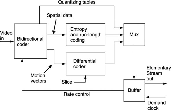
Figure 5.31 shows the complete coder. The bidirectional coder outputs coefficients and vectors, and the quantizing table in use. The vectors of P and B pictures and the DC coefficients of I pictures are differentially encoded in slices and the remaining coefficients are RLC/VLC coded. The multiplexer assembles all these data into a single bitstream called an elementary stream. The output of the encoder is a buffer which absorbs the variations in bit rate between different picture types. The buffer output has a constant bit rate determined by the demand clock. This comes from the transmission channel or storage device. If the bit rate is low, the buffer will tend to fill up, whereas if it is high the buffer will tend to empty. The buffer content is used to control the severity of the requantizing in the spatial coders. The more the buffer fills, the bigger the requantizing steps get.

Figure 5.31 An MPEG 2 coder. See text for details.

The buffer in the decoder has a finite capacity and the encoder must model the decoder’s buffer occupancy so that it neither overflows nor underflows. An overflow might occur if an I picture is transmitted when the buffer content is already high. The buffer occupancy of the decoder depends somewhat on the memory access strategy of the decoder. Instead of defining a specific buffer size, MPEG-2 defines the size of a particular mathematical model of a hypothetical buffer. The decoder designer can use any strategy which implements the model, and the encoder can use any strategy which doesn’t overflow or underflow the model. The elementary stream has a parameter called the video buffer verifier (VBV) which defines the minimum buffering assumptions of the encoder.

Buffering is one way of ensuring constant quality when picture entropy varies. An intelligent coder may run down the buffer contents in anticipation of a difficult picture sequence so that a large amounts of data can be sent.

MPEG-2 does not define what a decoder should do if a buffer underflow or overflow occurs, but since both irrecoverably lose data it is obvious that there will be more or less of an interruption to the decoding. Even a small loss of data may cause loss of synchronization and in the case of long GOP the lost data may make the rest of the GOP undecodable. A decoder may chose to repeat the last properly decoded picture until it can begin to operate correctly again.

Buffer problems occur if the VBV model is violated. If this happens then more than one underflow or overflow can result from a single violation. Switching an MPEG bitstream can cause a violation because the two encoders concerned may have radically different buffer occupancy at the switch.

5.10 The elementary stream

Figure 5.32 shows the structure of the elementary stream from an MPEG-2 encoder. The structure begins with a set of coefficients representing a DCT block. Six or eight DCT blocks form the luminance and chroma content of one macroblock. In P and B pictures a macroblock will be associated with a vector for motion compensation. Macroblocks are associated into slices in which DC coefficients of I pictures and vectors in P and B pictures are differentially coded. An arbitrary number of slices forms a picture and this needs I/P/B flags describing the type of picture it is. The picture may also have a global vector which efficiently deals with pans.

Figure 5.32 The structure of an elementary stream. MPEG defines the syntax precisely.

Several pictures form a GOP. The GOP begins with an I picture and may or may not include P and B pictures in a structure which may vary dynamically.

Several GOPs form a Sequence which begins with a Sequence header containing important data to help the decoder. It is possible to repeat the header within a sequence, and this helps lock-up in random access applications. The Sequence header describes the MPEG-2 profile and level, whether the video is progressive or interlaced, whether the chroma is 4:2:0 or 4:2:2, the size of the picture and the aspect ratio of the pixels. The quantizing matrix used in the spatial coder can also be sent. The sequence begins with a standardized bit pattern which is detected by a decoder to synchronize the deserialization.

5.11 An MPEG-2 decoder

The decoder is only defined by implication from the definitions of syntax and any decoder which can correctly interpret all combinations of syntax at a particular profile will be deemed compliant however it works.

The first problem a decoder has is that the input is an endless bitstream which contains a huge range of parameters many of which have variable length. Unique synchronizing patterns must be placed periodically throughout the bitstream so that the decoder can identify a known starting point. The pictures which can be sent under MPEG-2 are so flexible that the decoder must first find a Sequence header so that it can establish the size of the picture, the frame rate, the colour coding used, etc.

The decoder must also be supplied with a 27 MHz system clock. In a DVD player, this would come from a crystal, but in a transmission system this would be provided by a numerically locked loop running from a clock reference parameter in the bitstream (see Chapter 9). Until this loop has achieved lock the decoder cannot function properly.

Figure 5.33 shows a bidirectional decoder. The decoder can only begin decoding with an I picture and as this only uses intra-coding there will be no vectors. An I picture is transmitted as a series of slices. These slices begin with subsidiary synchronizing patterns. The first macroblock in the slice contains an absolute DC coefficient, but the remaining macroblocks code the DC coefficient differentially so the decoder must subtract the differential values from the previous value to obtain the absolute value.

Figure 5.33 A bidirectional MPEG-2 decoder. See text for details.

The AC coefficients are sent as Huffman coded run/size parameters followed by coefficient value codes. The variable-length Huffman codes are decoded by using a look-up table and extending the number of bits considered until a match is obtained. This allows the zero-run-length and the coefficient size to be established. The right number of bits is taken from the bitstream corresponding to the coefficient code and this is decoded to the actual coefficient using the size parameter.

If the correct number of bits has been taken from the stream, the next bit must be the beginning of the next run/size code and so on until the EOB (end of block) symbol is reached. The decoder uses the coefficient values and the zero-run-lengths to populate a DCT coefficient block following the appropriate zig-zag scanning sequence. Following EOB, the bitstream then continues with the next DCT block. Clearly this Huffman decoding will work perfectly or not at all. A single bit slippage in synchronism or a single corrupted data bit can cause a spectacular failure.

Once a complete DCT coefficient block has been received, the coefficients need to be inverse quantized and inverse weighted. Then an inverse DCT can be performed and this will result in an 8 × 8 pixel block. A series of DCT blocks will allow the luminance and colour information for an entire macroblock to be decoded and this can be placed in a framestore. Decoding continues in this way until the end of the slice when an absolute DC coefficient will once again be sent. Once all the slices have been decoded, an entire picture will be resident in the framestore.

The amount of data needed to decode the picture is variable and the decoder just keeps going until the last macroblock is found. It will obtain data from the input buffer. In a constant bit rate transmission system, the decoder will remove more data to decode an I picture than has been received in one picture period, leaving the buffer emptier than it began. Subsequent P and B pictures need much less data and allow the buffer to fill again. The picture will be output when the time stamp (see Chapter 9) sent with the picture matches the state of the decoder’s time count.

Following the I picture may be another I picture or a P picture. Assuming a P picture, this will be predictively coded from the I picture. The P picture will be divided into slices as before. The first vector in a slice is absolute, but subsequent vectors are sent differentially. However, the DC coefficients are not differential.

Each macroblock may contain a forward vector. The decoder uses this to shift pixels from the I picture into the correct position for the predicted P picture. The vectors have half-pixel resolution and where a half-pixel shift is required, an interpolator will be used.

The DCT data are sent much as for an I picture. They will require inverse quantizing, but not inverse weighting because P and B coefficients are flat-weighted. When decoded this represents an error-cancelling picture which is added pixel-by-pixel to the motion predicted picture. This results in the output picture.

If bidirectional coding is being used, the P picture may be stored until one or more B pictures have been decoded. The B pictures are sent essentially as a P picture might be, except that the vectors can be forward, backward or bidirectional. The decoder must take pixels from the I picture, the P picture, or both, and shift them according to the vectors to make a predicted picture. The DCT data decode to produce an error-cancelling image as before.

In an interlaced system, the prediction mechanism may alternatively obtain pixel data from the previous field or the field before that. Vectors may relate to macroblocks or to 16 × 8 pixel areas. DCT blocks after decoding may represent frame lines or field lines. This adds up to a lot of different possibilities for a decoder handling an interlaced input.

5.12 Coding artifacts

This section describes the visible results of imperfect coding. Imperfect coding may be where the coding algorithm is sub-optimal, where the coder latency is too short or where the compression factor in use is simply too great for the material.

In motion-compensated systems such as MPEG, the use of periodic intra-fields means that the coding noise varies from picture to picture and this may be visible as noise pumping. Noise pumping may also be visible where the amount of motion changes. If a pan is observed, as the pan speed increases the motion vectors may become less accurate and reduce the quality of the prediction processes. The prediction errors will get larger and will have to be more coarsely quantized. Thus the picture gets noisier as the pan accelerates and the noise reduces as the pan slows down. The same result may be apparent at the edges of a picture during zooming. The problem is worse if the picture contains fine detail. Panning on grass or trees waving in the wind taxes most coders severely. Camera shake from a hand-held camera also increases the motion vector data and results in more noise as does film weave.

Input video noise or film grain degrades inter-coding as there is less redundancy between pictures and the difference data become larger, requiring coarse quantizing and adding to the existing noise.

Where a codec is really fighting the quantizing may become very coarse and as a result the video level at the edge of one DCT block may not match that of its neighbour. As a result, the DCT block structure becomes visible as a mosaicing or tiling effect. Coarse quantizing also causes some coefficients to be rounded up and appear larger than they should be. High-frequency coefficients may be eliminated by heavy quantizing and this forces the DCT to act as a steepcut low-pass filter. This causes fringeing or ringing around sharp edges and extra shadowy edges which were not in the original. This is most noticeable on text.

Excess compression may also result in colour bleed where fringeing has taken place in the chroma or where high-frequency chroma coefficients have been discarded. Graduated colour areas may reveal banding or posterizing as the colour range is restricted by requantizing. These artifacts are almost impossible to measure with conventional test gear.

Neither noise pumping nor blocking are visible on analog video recorders and so it is nonsense to liken the performance of a codec to the quality of a VCR. In fact noise pumping is extremely objectionable because, unlike steady noise, it attracts attention in peripheral vision and may result in viewing fatigue.

In addition to highly detailed pictures with complex motion, certain types of video signal are difficult for MPEG-2 to handle and will usually result in a higher level of artifacts than usual. Noise has already been mentioned as a source of problems. Timebase error from, for example, VCRs is undesirable because this puts succesive lines in different horizontal positions. A straight vertical line becomes jagged and this results in high spatial frequencies in the DCT process. Spurious coefficients are created which need to be coded.

Much archive video is in composite form and MPEG-2 can only handle this after it has been decoded to components. Unfortunately many general-purpose composite decoders have a high level of residual subcarrier in the outputs. This is normally not a problem because the subcarrier is designed to be invisible to the naked eye. Figure 5.34 shows that in PAL and NTSC the subcarrier frequency is selected so that a phase reversal is achieved between successive lines and frames.

Figure 5.34 In composite video the subcarrier frequency is arranged so that inversions occur between adjacent lines and pictures to help reduce the visibility of the chroma.

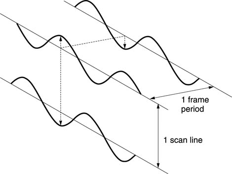
Whilst this makes the subcarrier invisible to the eye, it is not invisible to an MPEG decoder. The subcarrier waveform is interpreted as a horizontal frequency, the vertical phase reversals are interpreted as a vertical spatial frequency and the picture-to-picture reversals increase the magnitude of the prediction errors. The subcarrier level may be low but it can be present over the whole screen and require an excess of coefficients to describe it.

Composite video should not in general be used as a source for MPEG-2 encoding, but where this is inevitable the standard of the decoder must be much higher than average, especially in the residual subcarrier specification. Some MPEG preprocessors support high-grade composite decoding options.

Judder from conventional linear standards convertors degrades the performance of MPEG-2. The optic flow axis is corrupted and linear filtering causes multiple images which confuse motion estimators and result in larger prediction errors. If standards conversion is necessary, the MPEG-2 system must be used to encode the signal in its original format and the standards convertor should be installed after the decoder. If a standards convertor has to be used before the encoder, then it must be a type which has effective motion compensation.

Film weave causes movement of one picture with respect to the next and this results in more vector activity and larger prediction errors. Movement of the centre of the film frame along the optical axis causes magnification changes which also result in excess prediction error data. Film grain has the same effect as noise: it is random and so cannot be compressed.

Perhaps because it is relatively uncommon, MPEG-2 cannot handle image rotation well because the motion-compensation system is only designed for translational motion. Where a rotating object is highly detailed, such as in certain fairground rides, the motion-compensation failure requires a significant amount of prediction error data and if a suitable bit rate is not available the level of artifacts will rise.

Flash guns used by still photographers are a serious hazard to MPEG-2 especially when long GOPs are used. At a press conference where a series of flashes may occur, the resultant video contains intermittent white frames which defeat prediction. A huge prediction error is required to return to the original picture from a white picture. The output buffer fills and heavy requantizing is employed. After a few flashes the picture has generally gone to tiles.

5.13 Processing MPEG-2 and concatenation

Concatenation loss occurs when the losses introduced by one codec are compounded by a second codec. All practical compressers, MPEG-2 included, are lossy because what comes out of the decoder is not bit-identical to what went into the encoder. The bit differences are controlled so that they have minimum visibility to a human viewer.

MPEG-2 is a toolbox which allows a variety of manipulations to be performed in both the spatial and the temporal domains. There is a limit to the compression which can be used on a single frame, and if higher compression factors are needed, temporal coding will have to be used. The longer the run of pictures considered, the lower the bit rate needed, but the harder it becomes to edit.

The most editable form of MPEG-2 is to use I pictures only. As there is no temporal coding, pure cut edits can be made between pictures. The next best thing is to use a repeating IB structure which is locked to the odd/even field structure. Cut edits cannot be made as the B pictures are bidirectionally coded and need data from both adjacent I pictures for decoding. The B picture has to be decoded prior to the edit and re-encoded after the edit. This will cause a small concatenation loss.

Beyond the IB structure processing gets harder. If a long GOP is used for the best compression factor, an IBBPBBP … structure results. Editing this is very difficult because the pictures are sent out of order so that bidirectional decoding can be used. MPEG allows closed GOPs where the last B picture is coded wholly from the previous pictures and does not need the I picture in the next GOP. The bitstream can be switched at this point but only if the GOP structures in the two source video signals are synchronized (makes colour framing seem easy). Consequently in practice a long GOP bitstream will need to be decoded prior to any production step. Afterwards it will need to be re-encoded.

This is known as naive concatenation and an enormous pitfall awaits. Unless the GOP structure of the output is identical to and synchronized with the input the results will be disappointing. The worst case is where an I picture is encoded from a picture which was formerly a B picture. It is easy enough to lock the GOP structure of a coder to a single input, but if an edit is made between two inputs, the GOP timings could well be different.

As there are so many structures allowed in MPEG, there will be a need to convert between them. If this has to be done, it should only be in the direction which increases the GOP length and reduces the bit rate. Going the other way is inadvisable. The ideal way of converting from, say, the IB structure of a news system to the IBBP structure of an emission system is to use a recompressor. This is a kind of standards convertor which will give better results than a decode followed by an encode.

The DCT part of MPEG-2 itself is lossless. If all the coefficients are preserved intact an inverse transform yields the same pixel data. Unfortunately this does not yield enough compression for many applications. In practice the coefficients are made less accurate by removing bits starting at the least significant end and working upwards. This process is weighted, or made progressively more aggressive as spatial frequency increases.

Small-value coefficients may be truncated to zero and large-value coefficients are most coarsely truncated at high spatial frequencies where the effect is least visible.

Figure 5.35(a) shows what happens in the ideal case where two identical coders are put in tandem and synchronized. The first coder quantizes the coefficients to finite accuracy and causes a loss on decoding. However, when the second coder performs the DCT calculation, the coefficients obtained will be identical to the quantized coefficients in the first coder and so if the second weighting and requantizing step is identical the same truncated coefficient data will result and there will be no further loss of quality.7

Figure 5.35 (a) Two identical coders in tandem which are synchronized make similar coding decisions and cause little loss. (b) There are various ways in which concatenated coders can produce non-ideal performance.

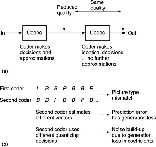
In practice this ideal situation is elusive. If the two DCTs become non-identical for any reason, the second requantizing step will introduce further error in the coefficients and the artifact level goes up. Figure 5.35(b) shows that non-identical concatenation can result from a large number of real-world effects.

An intermediate processing step such as a fade will change the pixel values and thereby the coefficients. A DVE resize or shift will move pixels from one DCT block to another. Even if there is no processing step, this effect will also occur if the two codecs disagree on where the MPEG picture boundaries are within the picture. If the boundaries are correct there will still be concatenation loss if the two codecs use different weightings.

One problem with MPEG is that the compressor design is unspecified. Whilst this has advantages, it does mean that the chances of finding identical coders is minute because each manufacturer will have their own views on the best compression algorithm. In a large system it may be worth obtaining the coders from a single supplier.

It is now increasingly accepted that concatenation of compression techniques is potentially damaging, and results are worse if the codecs are different. Clearly, feeding a digital coder such as MPEG-2 with a signal which has been subject to analog compression comes into the category of worse. Using interlaced video as a source for MPEG coding is sub-optimal and using decoded composite video is even worse.

One way of avoiding concatenation is to stay in the compressed data domain. If the goal is just to move pictures from one place to another, decoding to traditional video so an existing router can be used is not ideal, although substantially better than going through the analog domain.

Figure 5.36 shows some possibilities for picture transport. Clearly, if the pictures exist as a compressed file on a server, a file transfer is the right way to do it as there is no possibility of loss because there has been no concatenation. File transfer is also quite indifferent to the picture format. It doesn’t care whether the pictures are interlaced or not, whether the colour is 4:2:0 or 4:2:2.

Decoding to SDI (serial digital interface) standard is sometimes done so that existing serial digital routing can be used. This is concatenation and has to be done carefully. The compressed video can only use interlace with non-square pixels and the colour coding has to be 4:2:2 because SDI only allows that. If a compressed file has 4:2:0 the chroma has to be interpolated up to 4:2:2 for SDI transfer and then subsampled back to 4:2:0 at the second coder and this will cause generation loss. An SDI transfer also can only be performed in real time, thus negating one of the advantages of compression. In short, traditional SDI is not really at home with compression.

Figure 5.36 Compressed picture transport mechanisms contrasted.

As 4:2:0 progressive scan gains popularity and video production moves steadily towards non-format-specific hardware using computers and data networks, use of the serial digital interface will eventually decline. In the short term, if an existing SDI router has to be used, one solution is to produce a bitstream which is sufficiently similar to SDI that a router will pass it. In other words, the signal level, frequency and impedance is pure SDI, but the data protocol is different so that a bit-accurate file transfer can be performed. This has two advantages over SDI. First, the compressed data format can be anything appropriate and non-interlaced and/or 4:2:0 can be handled in any picture size, aspect ratio or frame rate. Second, a faster than real-time transfer can be used depending on the compression factor of the file. Equipment which allows this is becoming available and its use can mean that the full economic life of a SDI routing installation can be obtained.

An improved way of reducing concatenation loss has emerged from the ATLANTIC research project.8 Figure 5.37 shows that the second encoder in a concatenated scheme does not make its own decisions from the incoming video, but is instead steered by information from the first bitstream. As the second encoder has less intelligence, it is known as a dim encoder.

Figure 5.37 In an ATLANTIC system, the second encoder is steered by information from the decoder.

The information bus carries all the structure of the original MPEG-2 bitstream which would be lost in a conventional decoder. The ATLANTIC decoder does more than decode the pictures. It also places on the information bus all parameters needed to make the dim encoder re-enact what the initial MPEG-2 encode did as closely as possible.

The GOP structure is passed on so that pictures are re-encoded as the same type. Positions of macroblock boundaries become identical so that DCT blocks contain the same pixels and motion vectors relate to the same screen data. The weighting and quantizing tables are passed so that coefficient truncation is identical. Motion vectors from the original bitsream are passed on so that the dim encoder does not need to perform motion estimation. In this way predicted pictures will be identical to the original prediction and the prediction error data will be the same.

One application of this approach is in recompression, where an MPEG-2 bitstream has to have its bit rate reduced. This has to be done by heavier requantizing of coefficients, but if as many other parameters as possible can be kept the same, such as motion vectors, the degradation will be minimized. In a simple recompressor just requantizing the coefficients means that the predictive coding will be impaired. In a proper encode, the quantizing error due to coding, say, an I picture is removed from the P picture by the prediction process. The prediction error of P is obtained by subtracting the decoded I picture rather than the original I picture.

In simple recompression this does not happen and there may be a tolerance build-up known as drift.9 A more sophisticated recompressor will need to repeat the prediction process using the decoded output pictures as the prediction reference.

MPEG-2 bitstreams will often be decoded for the purpose of switching. Local insertion of commercial breaks into a centrally originated bitstream is one obvious requirement. If the decoded video signal is switched, the information bus must also be switched. At the switch point identical re-encoding becomes impossible because prior pictures required for predictive coding will have disappeared. At this point the dim encoder has to become bright again because it has to create an MPEG-2 bitstream without assistance.

It is possible to encode the information bus into a form which allows it to be invisibly carried in the serial digital interface. Where a production process such as a vision mixer or DVE performs no manipulation, i.e. becomes bit transparent, the subsequent encoder can extract the information bus and operate in ‘dim’ mode. Where a manipulation is performed, the information bus signal will be corrupted and the encoder has to work in ‘bright’ mode. The encoded information signal is known as a ‘mole’10 because it burrows through the processing equipment!

There will be a generation loss at the switch point because the re-encode will be making different decisions in bright mode. This may be difficult to detect because the human visual system is slow to react to a vision cut and defects in the first few pictures after a cut are masked.

In addition to the video computation required to perform a cut, the process has to consider the buffer occupancy of the decoder. A downstream decoder has finite buffer memory, and individual encoders model the decoder buffer occupancy to ensure that it neither overflows nor underflows. At any instant the decoder buffer can be nearly full or nearly empty without a problem provided there is a subsequent correction. An encoder which is approaching a complex I picture may run down the buffer so it can send a lot of data to describe that picture. Figure 5.38(a) shows that if a decoder with a nearly full buffer is suddenly switched to an encoder which has been running down its buffer occupancy, the decoder buffer will overflow when the second encoder sends a lot of data.

An MPEG-2 switcher will need to monitor the buffer occupancy of its own output to avoid overflow of downstream decoders. Where this is a possibility the second encoder will have to recompress to reduce the output bit rate temporarily. In practice there will be a recovery period where the buffer occupancy of the newly selected signal is matched to that of the previous signal. This is shown in Figure 5.38(b).

Figure 5.38 (a) A bitstream switch at a different level of buffer occupancy can cause a decoder overflow. (b) Recompression after a switch to return to correct buffer occupancy.

References

1. 1MPEG Video Standard: ISO/IEC 13818–2: Information technology – generic coding of moving pictures and associated audio information: Video (1996) (aka ITU-T Rec. H–262 (1996)

2. Huffman, D.A., A method for the construction of minimum redundancy codes. Proc. IRE, 40 1098–1101 (1952)

3. LeGall, D., MPEG: a video compression standard for multimedia applications. Communications of the ACM, 34, No.4, 46–58 (1991)

4. ISO/IEC JTC1/SC29/WG11 MPEG, International standard ISO 11172 ‘Coding of moving pictures and associated audio for digital storage media up to 1.5 Mbits/s’ (1992)

5. ISO Joint Photographic Experts Group standard JPEG–8-R8

6. Wallace, G.K., Overview of the JPEG (ISO/CCITT) still image compression standard. ISO/JTC1/SC2/WG8 N932 (1989)

7. 7.Stone, J. and Wilkinson, J., Concatenation of video compression systems. Presented at 137th SMPTE Tech Conf. New Orleans (1995)

8. Wells, N.D., The ATLANTIC project: Models for programme production and distribution. Proc. Euro. Conf. Multimedia Applications Services and Techniques (ECMAST), 243–253 (1996)

9. Werner, O., Drift analysis and drift reduction for multiresolution hybrid video coding. Image Communication, 8, 387–409 (1996)

10. 10.Knee, M.J. and Wells, N.D., Seamless concatenation – a 21st century dream. Presented at Int. Television. Symp. Montreux (1997)