Chapter 6

Digital coding principles

Recording and communication are quite different tasks, but they have a great deal in common. Digital transmission consists of converting data into a waveform suitable for the path along which they are to be sent. Digital recording is basically the process of recording a digital transmission waveform on a suitable medium. In this chapter the fundamentals of digital recording and transmission are introduced along with descriptions of the coding and error-correction techniques used in practical applications.

6.1 Introduction

Data can be recorded on many different media and conveyed using many forms of transmission. The generic term for the path down which the information is sent is the channel. In a transmission application, the channel may be a point-to-point cable, a network stage or a radio link. In a recording application the channel will include the record head, the medium and the replay head.

In digital circuitry there is a great deal of noise immunity because the signal has only two states, which are widely separated compared with the amplitude of noise. In both digital recording and transmission this is not always the case. In magnetic recording, noise immunity is a function of track width and reduction of the working SNR of a digital track allows the same information to be carried in a smaller area of the medium, improving economy of operation. In broadcasting, the noise immunity is a function of the transmitter power and reduction of working SNR allows lower power to be used with consequent economy. These reductions also increase the random error rate, but, as was seen in Chapter 1, an error-correction system may already be necessary in a practical system and it is simply made to work harder.

In real channels, the signal may originate with discrete states which change at discrete times, but the channel will treat it as an analog waveform and so it will not be received in the same form. Various frequency-dependent loss mechanisms will reduce the amplitude of the signal. Noise will be picked up as a result of stray electric fields or magnetic induction and in radio receivers the circuitry will contribute some noise. As a result, the received voltage will have an infinitely varying state along with a degree of uncertainty due to the noise. Different frequencies can propagate at different speeds in the channel; this is the phenomenon of group delay. An alternative way of considering group delay is that there will be frequency-dependent phase shifts in the signal and these will result in uncertainty in the timing of pulses.

In digital circuitry, the signals are generally accompanied by a separate clock signal which reclocks the data to remove jitter as was shown in Chapter 1. In contrast, it is generally not feasible to provide a separate clock in recording and transmission applications. In the transmission case, a separate clock line would not only raise cost, but is impractical because at high frequency it is virtually impossible to ensure that the clock cable propagates signals at the same speed as the data cable except over short distances. In the recording case, provision of a separate clock track is impractical at high density because mechanical tolerances cause phase errors between the tracks. The result is the same; timing differences between parallel channels which are known as skew.

The solution is to use a self-clocking waveform and the generation of this is a further essential function of the coding process. Clearly, if data bits are simply clocked serially from a shift register in so-called direct recording or transmission this characteristic will not be obtained. If all the data bits are the same, for example all zeros, there is no clock when they are serialized.

It is not the channel which is digital; instead the term describes the way in which the received signals are interpreted. When the receiver makes discrete decisions from the input waveform it attempts to reject the uncertainties in voltage and time. The technique of channel coding is one where transmitted waveforms are restricted to those which still allow the receiver to make discrete decisions despite the degradations caused by the analog nature of the channel.

6.2 Types of transmission channel

Transmission can be by electrical conductors, radio or optical fibre. Although these appear to be completely different, they are in fact just different examples of electromagnetic energy travelling from one place to another. If the energy is made time-variant, information can be carried.

Electromagnetic energy propagates in a manner which is a function of frequency, and our partial understanding requires it to be considered as electrons, waves or photons so that we can predict its behaviour in given circumstances.

At DC and at the low frequencies used for power distribution, electromagnetic energy is called electricity and needs to be transported completely inside conductors. It has to have a complete circuit to flow in, and the resistance to current flow is determined by the cross-sectional area of the conductor. The insulation around the conductor and the spacing between the conductors has no effect on the ability of the conductor to pass current. At DC an inductor appears to be a short circuit, and a capacitor appears to be an open circuit.

As frequency rises, resistance is exchanged for impedance. Inductors display increasing impedance with frequency, capacitors show falling impedance. Electromagnetic energy increasingly tends to leave the conductor. The first symptom is the skin effect: the current flows only in the outside layer of the conductor effectively causing the resistance to rise.

As the energy is starting to leave the conductors, the characteristics of the space between them become important. This determines the impedance. A change of impedance causes reflections in the energy flow and some of it heads back towards the source. Constant impedance cables with fixed conductor spacing are necessary, and these must be suitably terminated to prevent reflections. The most important characteristic of the insulation is its thickness as this determines the spacing between the conductors.

As frequency rises still further, the energy travels less in the conductors and more in the insulation between them, and their composition becomes important and they begin to be called dielectrics. A poor dielectric like PVC absorbs high-frequency energy and attenuates the signal. So-called low-loss dielectrics such as PTFE are used, and one way of achieving low loss is to incorporate as much air into the dielectric as possible by making it in the form of a foam or extruding it with voids.

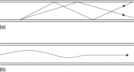
High-frequency signals can also be propagated without a medium, and are called radio. As frequency rises further the electromagnetic energy is termed ‘light’ which can also travel without a medium, but can be also be guided through a suitable medium. Figure 6.1(a) shows an early type of optical fibre in which total internal reflection is used to guide the light. It will be seen that the length of the optical path is a function of the angle at which the light is launched. Thus at the end of a long fibre sharp transitions would be smeared by this effect. Later optical fibres are made with a radially varying refractive index such that light diverging from the axis is automatically refracted back into the fibre. Figure 6.1(b) shows that in single-mode fibre light can only travel down one path and so the smearing of transitions is avoided.

Figure 6.1 (a) Early optical fibres operated on internal reflection, and signals could take a variety of paths along the fibre, hence multi-mode. (b) Later fibres used graduated refractive index which meant that light was guided to the centre of the fibre and only one mode was possible.

6.3 Transmission lines

Frequency-dependent behaviour is the most important factor in deciding how best to harness electromagnetic energy flow for information transmission. It is obvious that the higher the frequency, the greater the possible information rate, but in general, losses increase with frequency, and flat frequency response is elusive. The best that can be managed is that over a narrow band of frequencies, the response can be made reasonably constant with the help of equalization. Unfortunately raw data when serialized have an unconstrained spectrum. Runs of identical bits can produce frequencies much lower than the bit rate would suggest. One of the essential steps in a transmission system is to modify the spectrum of the data into something more suitable.

At moderate bit rates, say a few megabits per second, and with moderate cable lengths, say a few metres, the dominant effect will be the capacitance of the cable due to the geometry of the space between the conductors and the dielectric between. The capacitance behaves under these conditions as if it were a single capacitor connected across the signal. The effect of the series source resistance and the parallel capacitance is that signal edges or transitions are turned into exponential curves as the capacitance is effectively being charged and discharged through the source impedance.

As cable length increases, the capacitance can no longer be lumped as if it were a single unit; it has to be regarded as being distributed along the cable. With rising frequency, the cable inductance also becomes significant, and it too is distributed.

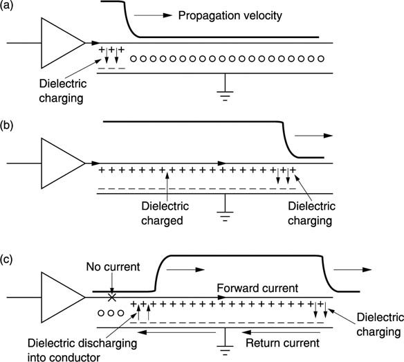
The cable is now a transmission line and pulses travel down it as current loops which roll along as shown in Figure 6.2. If the pulse is positive, as it is launched along the line, it will charge the dielectric locally as at (a). As the pulse moves along, it will continue to charge the local dielectric as at (b). When the driver finishes the pulse, the trailing edge of the pulse follows the leading edge along the line. The voltage of the dielectric charged by the leading edge of the pulse is now higher than the voltage on the line, and so the dielectric discharges into the line as at (c). The current flows forward as it is in fact the same current which is flowing into the dielectric at the leading edge. There is thus a loop of current rolling down the line flowing forward in the ‘hot’ wire and backwards in the return.

Figure 6.2 A transmission line conveys energy packets which appear with respect to the dielectric. In (a) the driver launches a pulse which charges the dielectric at the beginning of the line. As it propagates the dielectric is charged further along as in (b). When the driver ends the pulse, the charged dielectric discharges into the line. A current loop is formed where the current in the return loop flows in the opposite direction to the current in the ‘hot’ wire.

The constant to-ing and fro-ing of charge in the dielectric results in dielectric loss of signal energy. Dielectric loss increases with frequency and so a long transmission line acts as a filter. Thus the term ‘low-loss’ cable refers primarily to the kind of dielectric used.

Transmission lines which transport energy in this way have a characteristic impedance caused by the interplay of the inductance along the conductors with the parallel capacitance. One consequence of that transmission mode is that correct termination or matching is required between the line and both the driver and the receiver. When a line is correctly matched, the rolling energy rolls straight out of the line into the load and the maximum energy is available. If the impedance presented by the load is incorrect, there will be reflections from the mismatch. An open circuit will reflect all the energy back in the same polarity as the original, whereas a short circuit will reflect all the energy back in the opposite polarity. Thus impedances above or below the correct value will have a tendency towards reflections whose magnitude depends upon the degree of mismatch and whose polarity depends upon whether the load is too high or too low. In practice it is the need to avoid reflections which is the most important reason to terminate correctly.

A perfectly square pulse contains an indefinite series of harmonics, but the higher ones suffer progressively more loss. A square pulse at the driver becomes less and less square with distance as Figure 6.3 shows. The harmonics are progressively lost until in the extreme case all that is left is the fundamental. A transmitted square wave is received as a sine wave. Fortunately data can still be recovered from the fundamental signal component.

Figure 6.3 A signal may be square at the transmitter, but losses increase with frequency, and as the signal propagates, more of the harmonics are lost until only the fundamental remains. The amplitude of the fundamental then falls with further distance.

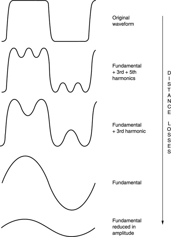
Once all the harmonics have been lost, further losses cause the amplitude of the fundamental to fall. The effect worsens with distance and it is necessary to ensure that data recovery is still possible from a signal of unpredictable level.

6.4 Types of recording medium

Digital media do not need to have linear transfer functions, nor do they need to be noise-free or continuous. All they need to do is to allow the player to be able to distinguish the presence or absence of replay events, such as the generation of pulses, with reasonable (rather than perfect) reliability. In a magnetic medium, the event will be a flux change from one direction of magnetization to another. In an optical medium, the event must cause the pickup to perceive a change in the intensity of the light falling on the sensor. This may be obtained through selective absorption of light by dyes, or by phase contrast (see Chapter 7). In magneto-optical disks the recording itself is magnetic, but it is made and read using light.

6.5 Magnetic recording

Magnetic recording relies on the hysteresis of certain magnetic materials. After an applied magnetic field is removed, the material remains magnetized in the same direction. By definition, the process is non-linear.

Figure 6.4 shows the construction of a typical digital record head. A magnetic circuit carries a coil through which the record current passes and generates flux. A non-magnetic gap forces the flux to leave the magnetic circuit of the head and penetrate the medium. The current through the head must be set to suit the coercivity of the tape, and is arranged to almost saturate the track. The amplitude of the current is constant, and recording is performed by reversing the direction of the current with respect to time. As the track passes the head, this is converted to the reversal of the magnetic field left on the tape with respect to distance. The magnetic recording is therefore bipolar. Figure 6.5 shows that the recording is actually made just after the trailing pole of the record head where the flux strength from the gap is falling. As in analog recorders, the width of the gap is generally made quite large to ensure that the full thickness of the magnetic coating is recorded, although this cannot be done if the same head is intended to replay.

Figure 6.4 A digital record head is similar in principle to an analog head but uses much narrower tracks.

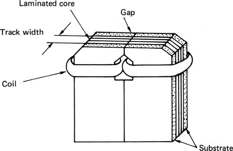
Figure 6.5 The recording is actually made near the trailing pole of the head where the head flux falls below the coercivity of the tape.

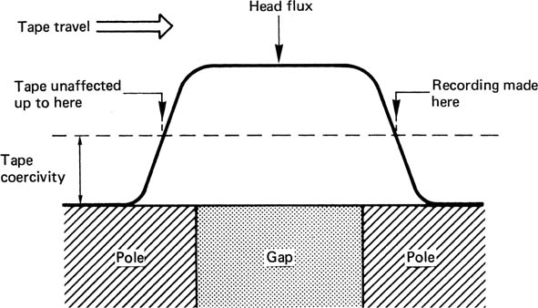
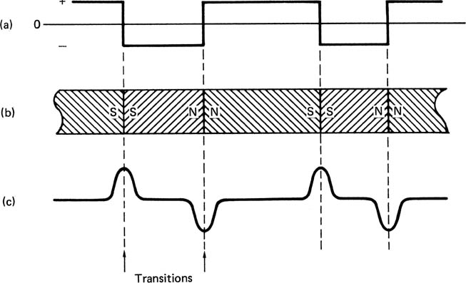
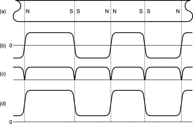
Figure 6.6 shows what happens when a conventional inductive head, i.e. one having a normal winding, is used to replay the bipolar track made by reversing the record current. The head output is proportional to the rate of change of flux and so only occurs at flux reversals. In other words, the replay head differentiates the flux on the track. The polarity of the resultant pulses alternates as the flux changes and changes back. A circuit is necessary which locates the peaks of the pulses and outputs a signal corresponding to the original record current waveform. There are two ways in which this can be done.

Figure 6.6 Basic digital recording. At (a) the write current in the head is reversed from time to time, leaving a binary magnetization pattern shown at (b). When replayed, the waveform at (c) results because an output is only produced when flux in the head changes. Changes are referred to as transitions.

The amplitude of the replay signal is of no consequence and often an AGC system is used to keep the replay signal constant in amplitude. What matters is the time at which the write current, and hence the flux stored on the medium, reverses. This can be determined by locating the peaks of the replay impulses, which can conveniently be done by differentiating the signal and looking for zero crossings. Figure 6.7 shows that this results in noise between the peaks. This problem is overcome by the gated peak detector, where only zero crossings from a pulse which exceeds the threshold will be counted. The AGC system allows the thresholds to be fixed. As an alternative, the record waveform can also be restored by integration, which opposes the differentiation of the head as in Figure 6.8.1

Figure 6.7 Gated peak detection rejects noise by disabling the differentiated output between transitions.

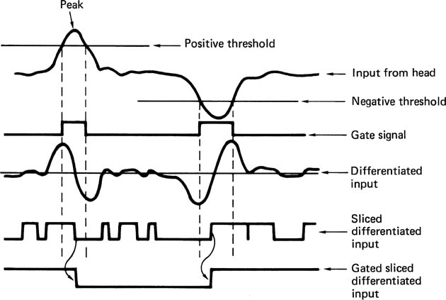
Figure 6.8 Integration method for re-creating write-current waveform.

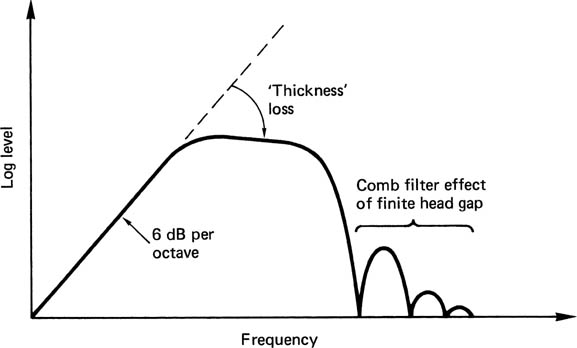
The head shown in Figure 6.4 has a frequency response shown in Figure 6.9. At DC there is no change of flux and no output. As a result, inductive heads are at a disadvantage at very low speeds. The output rises with frequency until the rise is halted by the onset of thickness loss. As the frequency rises, the recorded wavelength falls and flux from the shorter magnetic patterns cannot be picked up so far away. At some point, the wavelength becomes so short that flux from the back of the tape coating cannot reach the head and a decreasing thickness of tape contributes to the replay signal.2 In digital recorders using short wavelengths to obtain high density, there is no point in using thick coatings. As wavelength further reduces, the familiar gap loss occurs, where the head gap is too big to resolve detail on the track. The construction of the head results in the same action as that of a two-point transversal filter, as the two poles of the head see the tape with a small delay interposed due to the finite gap. As expected, the head response is like a comb filter with the well-known nulls where flux cancellation takes place across the gap. Clearly, the smaller the gap, the shorter the wavelength of the first null. This contradicts the requirement of the record head to have a large gap. In quality analog audio recorders, it is the norm to have different record and replay heads for this reason, and the same will be true in digital machines which have separate record and playback heads. Clearly, where the same heads are used for record and play, the head gap size will be determined by the playback requirement.

Figure 6.9 The major mechanisms defining magnetic channel bandwidth.

As can be seen, the frequency response is far from ideal, and steps must be taken to ensure that recorded data waveforms do not contain frequencies which suffer excessive losses.

A more recent development is the magneto-resistive (M-R) head. This is a head which measures the flux on the tape rather than using it to generate a signal directly. Flux-measurement works down to DC and so offers advantages at low tape speeds. Unfortunately flux-measuring heads are not polarity-conscious but sense the modulus of the flux and if used directly they respond to positive and negative flux equally, as shown in Figure 6.10. This is overcome by using a small extra winding in the head carrying a constant current. This creates a steady bias field which adds to the flux from the tape. The flux seen by the head is now unipolar and changes between two levels and a more useful output waveform results.

Recorders which have low head-to-medium speed use M-R heads, whereas recorders with high bit rates, such as DVTRs tend to use inductive heads.

Figure 6.10 The sensing element in a magneto-resistive head is not sensitive to the polarity of the flux, only the magnitude. At (a) the track magnetization is shown and this causes a bidirectional flux variation in the head as at (b), resulting in the magnitude output at (c). However, if the flux in the head due to the track is biased by an additional field, it can be made unipolar as at (d) and the correct waveform is obtained.

Heads designed for use with tape work in actual contact with the magnetic coating. The tape is tensioned to pull it against the head. There will be a wear mechanism and need for periodic cleaning. In the hard disk, the rotational speed is high in order to reduce access time, and the drive must be capable of staying on-line for extended periods. In this case the heads do not contact the disk surface, but are supported on a boundary layer of air. The presence of the air film causes spacing loss, which restricts the wavelengths at which the head can replay. This is the penalty of rapid access.

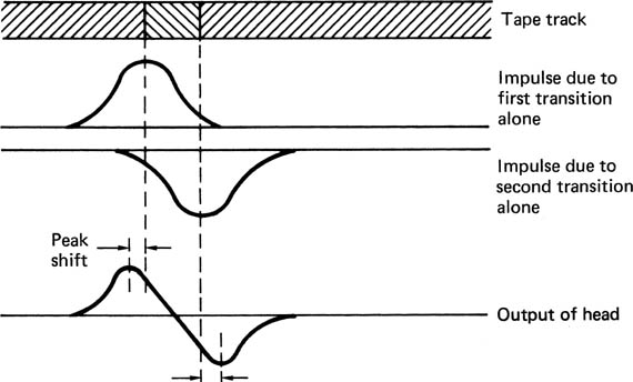
Digital media must operate at high density for economic reasons. This implies that the shortest possible wavelengths will be used. Figure 6.11 shows that when two flux changes, or transitions, are recorded close together, they affect each other on replay. The amplitude of the composite signal is reduced, and the position of the peaks is pushed outwards. This is known as inter-symbol interference, or peak-shift distortion and it occurs in all magnetic media.

Figure 6.11 Readout pulses from two closely recorded transitions are summed in the head and the effect is that the peaks of the waveform are moved outwards. This is known as peak-shift distortion and equalization is necessary to reduce the effect.

The effect is primarily due to high-frequency loss and it can be reduced by equalization on replay, as is done in most tapes, or by precompensation on record as is done in hard disks.

6.6 Azimuth recording and rotary heads

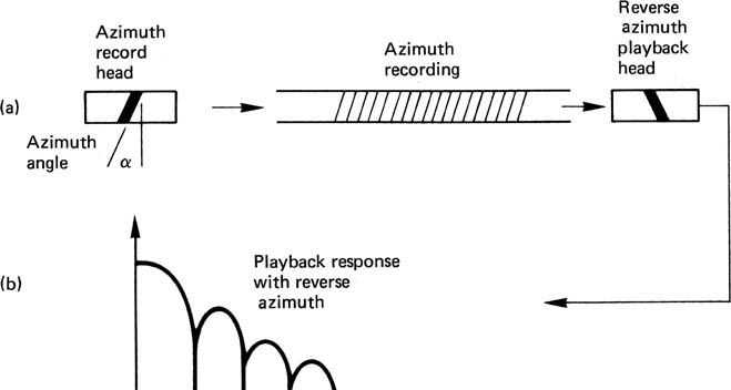
Figure 6.12(a) shows that in azimuth recording, the transitions are laid down at an angle to the track by using a head which is tilted. Machines using azimuth recording must always have an even number of heads, so that adjacent tracks can be recorded with opposite azimuth angle. The two track types are usually referred to as A and B. Figure 6.12(b) shows the effect of playing a track with the wrong type of head. The playback process suffers from an enormous azimuth error. The effect of azimuth error can be understood by imagining the tape track to be made from many identical parallel strips. In the presence of azimuth error, the strips at one edge of the track are played back with a phase shift relative to strips at the other side. At some wavelengths, the phase shift will be 180°, and there will be no output; at other wavelengths, especially long wavelengths, some output will reappear. The effect is rather like that of a comb filter, and serves to attenuate crosstalk due to adjacent tracks so that no guard bands are required. Since no tape is wasted between the tracks, more efficient use is made of the tape. The term ‘guard-bandless recording’ is often used instead of, or in addition to, ‘azimuth recording’. The failure of the azimuth effect at long wavelengths is a characteristic of azimuth recording, and it is necessary to ensure that the spectrum of the signal to be recorded has a small low-frequency content. The signal will need to pass through a rotary transformer to reach the heads, and cannot therefore contain a DC component.

Figure 6.12 In azimuth recording (a), the head gap is tilted. If the track is played with the same head, playback is normal, but the response of the reverse azimuth head is attenuated (b).

In some rotary head recorders there is no separate erase process, and erasure is achieved by overwriting with a new waveform. Overwriting is only successful when there are no long wavelengths in the earlier recording, since these penetrate deeper into the tape, and the short wavelengths in a new recording will not be able to erase them. In this case the ratio between the shortest and longest wavelengths recorded on tape should be limited.

Restricting the spectrum of the code to allow erasure by overwrite also eases the design of the rotary transformer.

6.7 Optical and magneto-optical disks

Optical recorders have the advantage that light can be focused at a distance whereas magnetism cannot. This means that there need be no physical contact between the pickup and the medium and no wear mechanism.

In the same way that the recorded wavelength of a magnetic recording is limited by the gap in the replay head, the density of optical recording is limited by the size of light spot which can be focused on the medium. This is controlled by the wavelength of the light used and by the aperture of the lens. When the light spot is as small as these limits allow, it is said to be diffraction limited.

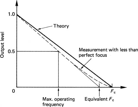
The frequency response of an optical disk is shown in Figure 6.13. The response is best at DC and falls steadily to the optical cut-off frequency. Although the optics work down to DC, this cannot be used for the data recording. DC and low frequencies in the data would interfere with the focus and tracking servos and, as will be seen, difficulties arise when attempting to demodulate a unipolar signal. In practice the signal from the pickup is split by a filter. Low frequencies go to the servos, and higher frequencies go to the data circuitry. As a result, the optical disk channel has the same inability to handle DC as does a magnetic recorder, and the same techniques are needed to overcome it.

Figure 6.13 Frequency response of laser pickup. Maximum operating frequency is about half of cut-off frequency F_c.

When a magnetic material is heated above its Curie temperature, it becomes demagnetized, and on cooling will assume the magnetization of an applied field which would be too weak to influence it normally. This is the principle of magneto-optical recording. The heat is supplied by a finely focused laser, the field is supplied by a coil which is much larger.

Figure 6.14 shows that the medium is initially magnetized in one direction only. In order to record, the coil is energized with a current in the opposite direction. This is too weak to influence the medium in its normal state, but when it is heated by the recording laser beam the heated area will take on the magnetism from the coil when it cools. Thus a magnetic recording with very small dimensions can be made even though the magnetic circuit involved is quite large in comparison.

Figure 6.14 The thermomagneto-optical disk uses the heat from a laser to allow magnetic field to record on the disk.

Readout is obtained using the Kerr effect or the Faraday effect, which are phenomena whereby the plane of polarization of light can be rotated by a magnetic field. The angle of rotation is very small and needs a sensitive pickup. The pickup contains a polarizing filter before the sensor. Changes in polarization change the ability of the light to get through the polarizing filter and results in an intensity change which once more produces a unipolar output.

The magneto-optic recording can be erased by reversing the current in the coil and operating the laser continuously as it passes along the track. A new recording can then be made on the erased track.

A disadvantage of magneto-optical recording is that all materials having a Curie point low enough to be useful are highly corrodible by air and need to be kept under an effectively sealed protective layer. The magneto-optical channel has the same frequency response as that shown in Figure 2.69.

6.8 Equalization and data separation

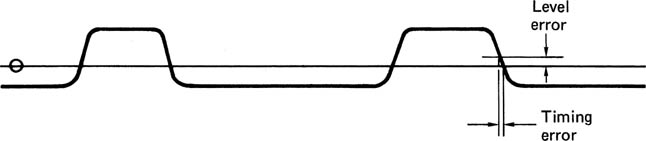
The characteristics of most channels are that signal loss occurs which increases with frequency. This has the effect of slowing down rise times and thereby sloping off edges. If a signal with sloping edges is sliced, the time at which the waveform crosses the slicing level will be changed, and this causes jitter. Figure 6.15 shows that slicing a sloping waveform in the presence of baseline wander causes more jitter.

Figure 6.15 A DC offset can cause timing errors.

On a long cable, high-frequency roll-off can cause sufficient jitter to move a transition into an adjacent bit period. This is called inter-symbol interference and the effect becomes worse in signals which have greater asymmetry, i.e. short pulses alternating with long ones. The effect can be reduced by the application of equalization, which is typically a high-frequency boost, and by choosing a channel code which has restricted asymmetry.

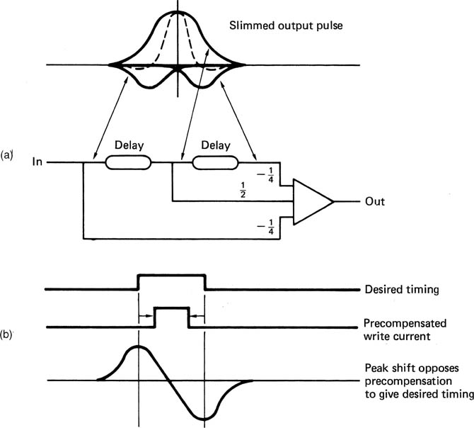
Compensation for peak shift distortion in recording requires equalization of the channel,3 and this can be done by a network after the replay head, termed an equalizer or pulse sharpener,4 as in Figure 6.16(a). This technique uses transversal filtering to oppose the inherent transversal effect of the head. As an alternative, precompensation in the record stage can be used as shown in Figure 6.16(b). Transitions are written in such a way that the anticipated peak shift will move the readout peaks to the desired timing.

Figure 6.16 Peak-shift distortion is due to the finite width of replay pulses. The effect can be reduced by the pulse slimmer shown in (a) which is basically a transversal filter. The use of a linear operational amplifier emphasizes the analog nature of channels. Instead of replay pulse slimming, transitions can be written with a displacement equal and opposite to the anticipated peak shift as shown in (b).

The important step of information recovery at the receiver or replay circuit is known as data separation. The data separator is rather like an analog-to-digital convertor because the two processes of sampling and quantizing are both present. In the time domain, the sampling clock is derived from the clock content of the channel waveform. In the voltage domain, the process of slicing converts the analog waveform from the channel back into a binary representation. The slicer is thus a form of quantizer which has only one-bit resolution. The slicing process makes a discrete decision about the voltage of the incoming signal in order to reject noise. The sampler makes discrete decisions along the time axis in order to reject jitter. These two processes will be described in detail.

6.9 Slicing and jitter rejection

The slicer is implemented with a comparator which has analog inputs but a binary output. In a cable receiver, the input waveform can be sliced directly. In an inductive magnetic replay system, the replay waveform is differentiated and must first pass through a peak detector (Figure 6.7) or an integrator (Figure 6.8). The signal voltage is compared with the midway voltage, known as the threshold, baseline or slicing level by the comparator. If the signal voltage is above the threshold, the comparator outputs a high level, if below, a low level results.

Figure 6.17 shows some waveforms associated with a slicer. At (a) the transmitted waveform has an uneven duty cycle. The DC component, or average level, of the signal is received with high amplitude, but the pulse amplitude falls as the pulse gets shorter. Eventually the waveform cannot be sliced.

Figure 6.17 Slicing a signal which has suffered losses works well if the duty cycle is even. If the duty cycle is uneven, as at (a), timing errors will become worse until slicing fails. With the opposite duty cycle, the slicing fails in the opposite direction as at (b). If, however, the signal is DC free, correct slicing can continue even in the presence of serious losses, as (c) shows.

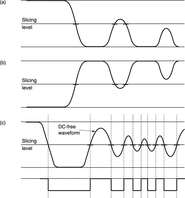
At (b) the opposite duty cycle is shown. The signal level drifts to the opposite polarity and once more slicing is impossible. The phenomenon is called baseline wander and will be observed with any signal whose average voltage is not the same as the slicing level.

At (c) it will be seen that if the transmitted waveform has a relatively constant average voltage, slicing remains possible up to high frequencies even in the presence of serious amplitude loss, because the received waveform remains symmetrical about the baseline.

It is clearly not possible simply to serialize data in a shift register for so-called direct transmission, because successful slicing can only be obtained if the number of ones is equal to the number of zeros; there is little chance of this happening consistently with real data. Instead, a modulation code or channel code is necessary. This converts the data into a waveform which is DC-free or nearly so for the purpose of transmission.

The slicing threshold level is naturally zero in a bipolar system such as magnetic inductive replay or a cable. When the amplitude falls it does so symmetrically and slicing continues. The same is not true of M-R heads and optical pickups, which both respond to intensity and therefore produce a unipolar output. If the replay signal is sliced directly, the threshold cannot be zero, but must be some level approximately half the amplitude of the signal as shown in Figure 6.18(a). Unfortunately when the signal level falls it falls towards zero and not towards the slicing level. The threshold will no longer be appropriate for the signal as can be seen at (b). This can be overcome by using a DC-free coded waveform. If a series capacitor is connected to the unipolar signal from an optical pickup, the waveform is rendered bipolar because the capacitor blocks any DC component in the signal. The DC-free channel waveform passes through unaltered. If an amplitude loss is suffered, Figure 6.18(c) shows that the resultant bipolar signal now reduces in amplitude about the slicing level and slicing can continue.

Figure 6.18 (a) Slicing a unipolar signal requires a non-zero threshold. (b) If the signal amplitude changes, the threshold will then be incorrect. (c) If a DC-free code is used, a unipolar waveform can be converted to a bipolar waveform using a series capacitor. A zero threshold can be used and slicing continues with amplitude variations.

The binary waveform at the output of the slicer will be a replica of the transmitted waveform, except for the addition of jitter or time uncertainty in the position of the edges due to noise, baseline wander, intersymbol interference and imperfect equalization.

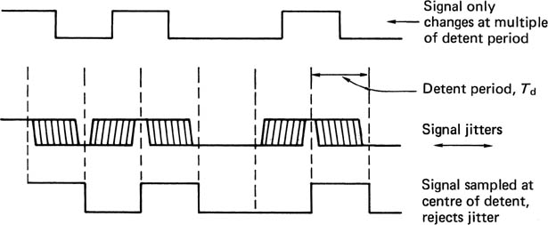
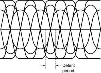
Binary circuits reject noise by using discrete voltage levels which are spaced further apart than the uncertainty due to noise. In a similar manner, digital coding combats time uncertainty by making the time axis discrete using events, known as transitions, spaced apart at integer multiples of some basic time period, called a detent, which is larger than the typical time uncertainty. Figure 6.19 shows how this jitter-rejection mechanism works. All that matters is to identify the detent in which the transition occurred. Exactly where it occurred within the detent is of no consequence.

Figure 6.19 A certain amount of jitter can be rejected by changing the signal at multiples of the basic detent period T_d.

As ideal transitions occur at multiples of a basic period, an oscilloscope, which is repeatedly triggered on a channel-coded signal carrying random data, will show an eye pattern if connected to the output of the equalizer. Study of the eye pattern reveals how well the coding used suits the channel. In the case of transmission, with a short cable, the losses will be small, and the eye opening will be virtually square except for some edge-sloping due to cable capacitance. As cable length increases, the harmonics are lost and the remaining fundamental gives the eyes a diamond shape. The same eye pattern will be obtained with a recording channel where it is uneconomic to provide bandwidth much beyond the fundamental.

Noise closes the eyes in a vertical direction, and jitter closes the eyes in a horizontal direction, as in Figure 6.20. If the eyes remain sensibly open, data separation will be possible. Clearly, more jitter can be tolerated if there is less noise, and vice versa. If the equalizer is adjustable, the optimum setting will be where the greatest eye opening is obtained.

Figure 6.20 A transmitted waveform will appear like this on an oscilloscope as successive parts of the waveform are superimposed on the tube. When the waveform is rounded off by losses, diamond-shaped eyes are left in the centre, spaced apart by the detent period.

In the centre of the eyes, the receiver must make binary decisions at the channel bit rate about the state of the signal, high or low, using the slicer output. As stated, the receiver is sampling the output of the slicer, and it needs to have a sampling clock in order to do that. In order to give the best rejection of noise and jitter, the clock edges which operate the sampler must be in the centre of the eyes.

As has been stated, a separate clock is not practicable in recording or transmission. A fixed-frequency clock at the receiver is of no use as even if it was sufficiently stable, it would not know what phase to run at.

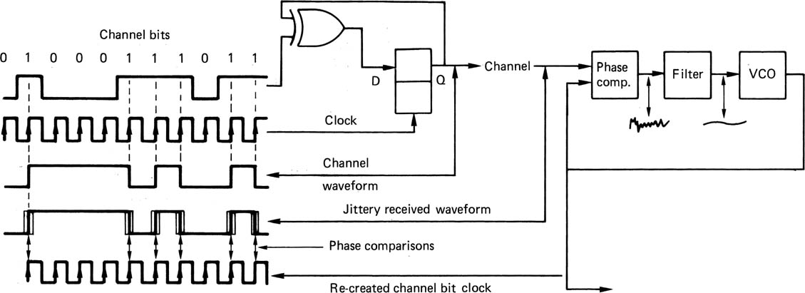
The only way in which the sampling clock can be obtained is to use a phase-locked loop to regenerate it from the clock content of the self-clocking channel-coded waveform. In phase-locked loops, the voltage-controlled oscillator is driven by a phase error measured between the output and some reference, such that the output eventually has the same frequency as the reference. If a divider is placed between the VCO and the phase comparator, as in section 2.9, the VCO frequency can be made to be a multiple of the reference. This also has the effect of making the loop more heavily damped. If a channel-coded waveform is used as a reference to a PLL, the loop will be able to make a phase comparison whenever a transition arrives and will run at the channel bit rate. When there are several detents between transitions, the loop will flywheel at the last known frequency and phase until it can rephase at a subsequent transition. Thus a continuous clock is re-created from the clock content of the channel waveform. In a recorder, if the speed of the medium should change, the PLL will change frequency to follow. Once the loop is locked, clock edges will be phased with the average phase of the jittering edges of the input waveform. If, for example, rising edges of the clock are phased to input transitions, then falling edges will be in the centre of the eyes. If these edges are used to clock the sampling process, the maximum jitter and noise can be rejected. The output of the slicer when sampled by the PLL edge at the centre of an eye is the value of a channel bit. Figure 6.21 shows the complete clocking system of a channel code from encoder to data separator.

Figure 6.21 The clocking system when channel coding is used. The encoder clock runs at the channel bit rate, and any transitions in the channel must coincide with encoder clock edges. The reason for doing this is that, at the data separator, the PLL can lock to the edges of the channel signal, which represents an intermittent clock, and turn it into a continuous clock. The jitter in the edges of the channel signal causes noise in the phase error of the PLL, but the damping acts as a filter and the PLL runs at the average phase of the channel bits, rejecting the jitter.

Clearly, data cannot be separated if the PLL is not locked, but it cannot be locked until it has seen transitions for a reasonable period. In recorders, which have discontinuous recorded blocks to allow editing, the solution is to precede each data block with a pattern of transitions whose sole purpose is to provide a timing reference for synchronizing the phase-locked loop. This pattern is known as a preamble. In interfaces, the transmission can be continuous and there is no difficulty remaining in lock indefinitely. There will simply be a short delay on first applying the signal before the receiver locks to it.

One potential problem area which is frequently overlooked is to ensure that the VCO in the receiving PLL is correctly centred. If it is not, it will be running with a static phase error and will not sample the received waveform at the centre of the eyes. The sampled bits will be more prone to noise and jitter errors. VCO centring can simply be checked by displaying the control voltage. This should not change significantly when the input is momentarily interrupted.

6.10 Channel coding

It is not practicable simply to serialize raw data in a shift register for the purpose of recording or for transmission except over relatively short distances. Practical systems require the use of a modulation scheme, known as a channel code, which expresses the data as waveforms which are self-clocking in order to reject jitter, separate the received bits and to avoid skew on separate clock lines. The coded waveforms should further be DC-free or nearly so to enable slicing in the presence of losses and have a narrower spectrum than the raw data both for economy and to make equalization easier.

Jitter causes uncertainty about the time at which a particular event occurred. The frequency response of the channel then places an overall limit on the spacing of events in the channel. Particular emphasis must be placed on the interplay of bandwidth, jitter and noise, which will be shown here to be the key to the design of a successful channel code.

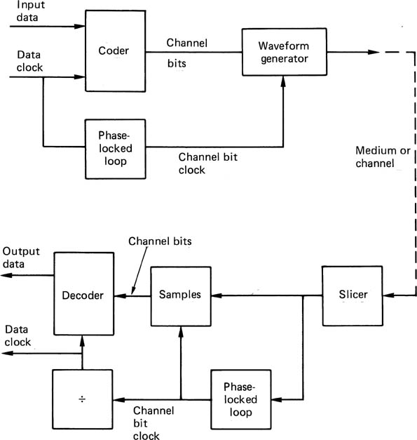
Figure 6.22 shows that a channel coder is necessary prior to the record stage, and that a decoder, known as a data separator, is necessary after the replay stage. The output of the channel coder is generally a logic-level signal which contains a ‘high’ state when a transition is to be generated. The waveform generator produces the transitions in a signal whose level and impedance is suitable for driving the medium or channel. The signal may be bipolar or unipolar as appropriate.

Figure 6.22 The major components of a channel coding system. See text for details.

Some codes eliminate DC entirely, which is advantageous for cable transmission, optical media and rotary head recording. Some codes can reduce the channel bandwidth needed by lowering the upper spectral limit. This permits higher linear density, usually at the expense of jitter rejection. Other codes narrow the spectrum, by raising the lower limit. A code with a narrow spectrum has a number of advantages. The reduction in asymmetry will reduce peak shift and data separators can lock more readily because the range of frequencies in the code is smaller. In theory the narrower the spectrum, the less noise will be suffered, but this is only achieved if filtering is employed. Filters can easily cause phase errors which will nullify any gain.

A convenient definition of a channel code (for there are certainly others) is ‘A method of modulating real data such that they can be reliably received despite the shortcomings of a real channel, while making maximum economic use of the channel capacity’. The basic time periods of a channel-coded waveform are called positions or detents, in which the transmitted voltage will be reversed or stay the same. The symbol used for the units of channel time is T_d.

One of the fundamental parameters of a channel code is the density ratio (DR). One definition of density ratio is that it is the worst-case ratio of the number of data bits recorded to the number of transitions in the channel. It can also be thought of as the ratio between the Nyquist rate of the data (one-half the bit rate) and the frequency response required in the channel. The storage density of data recorders has steadily increased due to improvements in medium and transducer technology, but modern storage densities are also a function of improvements in channel coding.

As jitter is such an important issue in digital recording and transmission, a parameter has been introduced to quantify the ability of a channel code to reject time instability. This parameter, the jitter margin, also known as the window margin or phase margin (T_w), is defined as the permitted range of time over which a transition can still be received correctly, divided by the data bit-cell period (T).

Since equalization is often difficult in practice, a code which has a large jitter margin will sometimes be used because it resists the effects of inter-symbol interference well. Such a code may achieve a better performance in practice than a code with a higher density ratio but poor jitter performance.

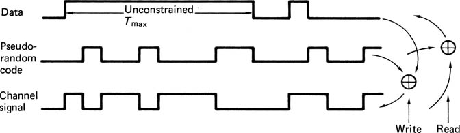
A more realistic comparison of code performance will be obtained by taking into account both density ratio and jitter margin. This is the purpose of the figure of merit (FoM), which is defined as DR × T_w.

6.11 Simple codes

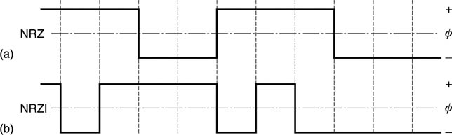
In the Non-Return to Zero (NRZ) code shown in Figure 6.23(a), the record current does not cease between bits, but flows at all times in one direction or the other dependent on the state of the bit to be recorded. This results in a replay pulse only when the data bits change from state to another. As a result, if one pulse was missed, the subsequent bits would be inverted. This was avoided by adapting the coding such that the record current would change state or invert whenever a data one occurred, leading to the term Non-Return to Zero Invert or NRZI shown in Figure 6.23b). In NRZI a replay pulse occurs whenever there is a data one. Clearly, neither NRZ or NRZI are self-clocking, but require a separate clock track. Skew between tracks can only be avoided by working at low density and so the system cannot be used directly for digital video. However, virtually all the codes used for magnetic recording are based on the principle of reversing the record current to produce a transition.

Figure 6.23 In the NRZ code (a) a missing replay pulse inverts every following bit. This was overcome in the NRZI code (b) which reverses write current on a data one.

The FM code, also known as Manchester code or bi-phase mark code, shown in Figure 6.24(a) was the first practical self-clocking binary code and it is suitable for both transmission and recording. It is DC-free and very easy to encode and decode. It is the code specified for the AES/EBU digital audio interconnect standard. In the field of recording it remains in use today only where density is not of prime importance, for example in SMPTE/EBU timecode for professional audio and video recorders.

In FM there is always a transition at the bit-cell boundary which acts as a clock. For a data one, there is an additional transition at the bit-cell centre. Figure 6.24(a) shows that each data bit can be represented by two channel bits. For a data zero, they will be 10, and for a data one they will be 11. Since the first bit is always one, it conveys no information, and is responsible for the density ratio of only one-half. Since there can be two transitions for each data bit, the jitter margin can only be half a bit, and the resulting FoM is only 0.25. The high clock content of FM does, however, mean that data recovery is possible over a wide range of speeds; hence the use of timecode. The lowest frequency in FM is due to a stream of zeros and is equal to half the bit rate. The highest frequency is due to a stream of ones, and is equal to the bit rate. Thus the fundamentals of FM are within a band of one octave. Effective equalization is generally possible over such a band. FM is not polarity-conscious and can be inverted without changing the data.

Figure 6.24 FM encoding. At (a) are the FM waveform and the channel bits which may be used to describe transitions in it. The FM coder is shown at (b).

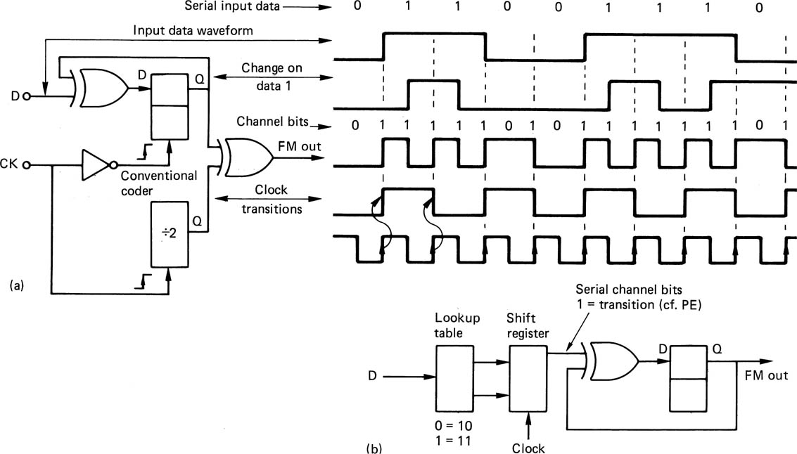
Figure 6.24(b) shows how an FM coder works. Data words are loaded into the input shift register which is clocked at the data bit rate. Each data bit is converted to two channel bits in the codebook or look-up table. These channel bits are loaded into the output register. The output register is clocked twice as fast as the input register because there are twice as many channel bits as data bits. The ratio of the two clocks is called the code rate, in this case it is a rate one-half code. Ones in the serial channel bit output represent transitions whereas zeros represent no change. The channel bits are fed to the waveform generator which is a one-bit delay, clocked at the channel bit rate, and an exclusive-OR gate. This changes state when a channel bit one is input. The result is a coded FM waveform where there is always a transition at the beginning of the data bit period, and a second optional transition whose presence indicates a one.

In modified frequency modulation (MFM) also known as Miller code,5 the highly redundant clock content of FM was reduced by the use of a phase-locked loop in the receiver which could flywheel over missing clock transitions. This technique is implicit in all the more advanced codes. Figure 6.25(a) shows that the bit-cell centre transition on a data one was retained, but the bit-cell boundary transition is now required only between successive zeros. There are still two channel bits for every data bit, but adjacent channel bits will never be one, doubling the minimum time between transitions, and giving a DR of 1. Clearly, the coding of the current bit is now influenced by the preceding bit. The maximum number of prior bits which affect the current bit is known as the constraint length L_c, measured in data-bit periods. For MFM L_c = T. Another way of considering the constraint length is that it assesses the number of data bits which may be corrupted if the receiver misplaces one transition. If Lc is long, all errors will be burst errors.

Figure 6.25 MFM or Miller code is generated as shown here. The minimum transition spacing is twice that of FM or PE. MFM is not always DC-free as shown at (b). This can be overcome by the modification of (c) which results in the Miller2 code.

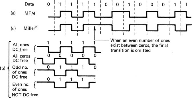
MFM doubled the density ratio compared to FM and PE without changing the jitter performance; thus the FoM also doubles, becoming 0.5. It was adopted for many rigid disks at the time of its development, and remains in use on double-density floppy disks. It is not, however, DC-free. Figure 6.25(b) shows how MFM can have DC content under certain conditions.

The Miller2 code is derived from MFM, and Figure 6.25(c) shows that the DC content is eliminated by a slight increase in complexity.6, 7 Wherever an even number of ones occurs between zeros, the transition at the last one is omitted. This creates two additional, longer run lengths and increases the T_max of the code. The decoder can detect these longer run lengths in order to re-insert the suppressed ones. The FoM of Miller2 is 0.5 as for MFM.

6.12 Group codes

Further improvements in coding rely on converting patterns of real data to patterns of channel bits with more desirable characteristics using a conversion table known as a codebook. If a data symbol of m bits is considered, it can have 2^m different combinations. As it is intended to discard undesirable patterns to improve the code, it follows that the number of channel bits n must be greater than m. The number of patterns which can be discarded is:

One name for the principle is group code recording (GCR), and an important parameter is the code rate, defined as:

It will be evident that the jitter margin T_w is numerically equal to the code rate, and so a code rate near to unity is desirable. The choice of patterns which are used in the codebook will be those which give the desired balance between clock content, bandwidth and DC content.

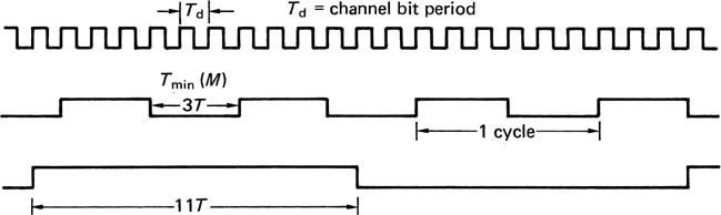
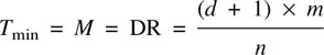
Figure 6.26 shows that the upper spectral limit can be made to be some fraction of the channel bit rate according to the minimum distance between ones in the channel bits. This is known as T_min, also referred to as the minimum transition parameter M and in both cases is measured in data bits T. It can be obtained by multiplying the number of channel detent periods between transitions by the code rate. Unfortunately, codes are measured by the number of consecutive zeros in the channel bits, given the symbol d, which is always one less than the number of detent periods. In fact T_min is numerically equal to the density ratio.

Figure 6.26 A channel code can control its spectrum by placing limits on T_min (M) and T_max which define upper and lower frequencies. The ratio of T_max/T_min determines the asymmetry of waveform and predicts DC content and peak shift. Example shown is EFM.

It will be evident that choosing a low code rate could increase the density ratio, but it will impair the jitter margin. The figure of merit is:

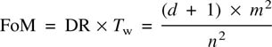
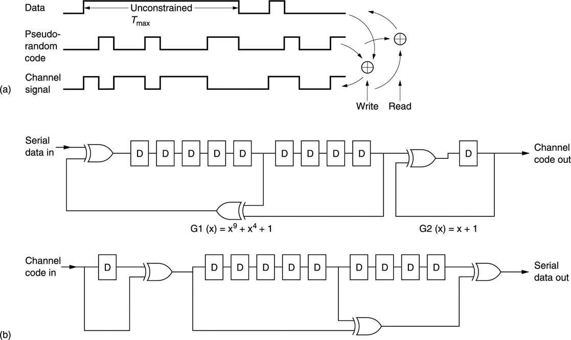
Figure 6.26 also shows that the lower spectral limit is influenced by the maximum distance between transitions T_max. This is also obtained by multiplying the maximum number of detent periods between transitions by the code rate. Again, codes are measured by the maximum number of zeros between channel ones, k, and so:

and the maximum/minimum ratio P is:

The length of time between channel transitions is known as the run length. Another name for this class is the run-length-limited (RLL) codes.8 Since m data bits are considered as one symbol, the constraint length L_c will be increased in RLL codes to at least m. It is, however, possible for a code to have run-length limits without it being a group code.

In practice, the junction of two adjacent channel symbols may violate run-length limits, and it may be necessary to create a further codebook of symbol size 2n which converts violating code pairs to acceptable patterns. This is known as merging and follows the golden rule that the substitute 2n symbol must finish with a pattern which eliminates the possibility of a subsequent violation. These patterns must also differ from all other symbols.

Substitution may also be used to different degrees in the same nominal code in order to allow a choice of maximum run length, e.g. 3PM. The maximum number of symbols involved in a substitution is denoted by r. There are many RLL codes and the parameters d, k, m, n, and r are a way of comparing them.

Group codes are used extensively in recording and transmission. DVTRs and magnetic disks use group codes optimized for jitter rejection whereas optical disks use group codes optimized for density ratio.

6.13 Randomizing and encryption

Randomizing is not a channel code, but a technique which can be used in conjunction with almost any channel code. It is widely used in digital audio and video broadcasting and in a number of recording and transmission formats. The randomizing system is arranged outside the channel coder. Figure 6.27 shows that, at the encoder, a pseudo-random sequence is added modulo-2 to the serial data. This process makes the signal spectrum in the channel more uniform, drastically reduces T_max and reduces DC content. At the receiver the transitions are converted back to a serial bitstream to which the same pseudo-random sequence is again added modulo-2. As a result, the random signal cancels itself out to leave only the serial data, provided that the two pseudo-random sequences are synchronized to bit accuracy.

Figure 6.27 Modulo-2 addition with a pseudo-random code removes unconstrained runs in real data. Identical process must be provided on replay.

Many channel codes, especially group codes, display pattern sensitivity because some waveforms are more sensitive to peak shift distortion than others. Pattern sensitivity is only a problem if a sustained series of sensitive symbols needs to be recorded. Randomizing ensures that this cannot happen because it breaks up any regularity or repetition in the data. The data randomizing is performed by using the exclusive-OR function of the data and a pseudo-random sequence as the input to the channel coder. On replay the same sequence is generated, synchronized to bit accuracy, and the exclusive-OR of the replay bitstream and the sequence is the original data.

The generation of randomizing polynomials was described in section 2.8. Clearly, the sync pattern cannot be randomized, since this causes a Catch_22 situation where it is not possible to synchronize the sequence for replay until the sync pattern is read, but it is not possible to read the sync pattern until the sequence is synchronized!

In recorders, the randomizing is block based, since this matches the block structure on the medium. Where there is no obvious block structure, convolutional or endless randomizing can be used. In convolutional randomizing, the signal sent down the channel is the serial data waveform which has been convolved with the impulse response of a digital filter. On reception the signal is deconvolved to restore the original data.

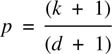
Convolutional randomizing is used in the serial digital interface (SDI) which carries 4:2:2 sampled video. Figure 6.28(a) shows that the filter is an infinite impulse response (IIR) filter which has recursive paths from the output back to the input. As it is a one-bit filter its output cannot decay, and once excited, it runs indefinitely. The filter is followed by a transition generator which consists of a one-bit delay and an exclusive-OR gate. An input 1 results in an output transition on the next clock edge. An input 0 results in no transition.

Figure 6.28 (a) Modulo-2 addition with a pseudo-random code removes unconstrained runs in real data. Identical process must be provided on replay. (b) Convolutional randomizing encoder, at top, transmits exclusive-OR of three bits at a fixed spacing in the data. One bit delay, far right, produces channel transitions from data ones. Decoder, below, has opposing one bit delay to return from transitions to data levels, followed by an opposing shift register which exactly reverses the coding process.

A result of the infinite impulse response of the filter is that frequent transitions are generated in the channel which result in sufficient clock content for the phase-locked loop in the receiver.

Transitions are converted back to 1s by a differentiator in the receiver. This consists of a one-bit delay with an exclusive-OR gate comparing the input and the output. When a transition passes through the delay, the input and the output will be different and the gate outputs a 1 which enters the deconvolution circuit.

Figure 6.28(b) shows that in the deconvolution circuit a data bit is simply the exclusive-OR of a number of channel bits at a fixed spacing. The deconvolution is implemented with a shift register having the exclusive-OR gates connected in a reverse pattern to that in the encoder. The same effect as block randomizing is obtained, in that long runs are broken up and the DC content is reduced, but it has the advantage over block randomizing that no synchronizing is required to remove the randomizing, although it will still be necessary for deserialization. Clearly, the system will take a few clock periods to produce valid data after commencement of transmission, but this is no problem on a permanent wired connection where the transmission is continuous.

In a randomized transmission, if the receiver is not able to re-create the pseudo-random sequence, the data cannot be decoded. This can be used as the basis for encryption in which only authorized users can decode transmitted data. In an encryption system, the goal is security whereas in a channel-coding system the goal is simplicity. Channel coders use pseudo-random sequences because these are economical to create using feedback shift registers. However, there are a limited number of pseudo-random sequences and it would be too easy to try them all until the correct one was found. Encryption systems use the same processes, but the key sequence which is added to the data at the encoder is truly random. This makes it much harder for unauthorized parties to access the data. Only a receiver in possession of the correct sequence can decode the channel signal. If the sequence is made long enough, the probability of stumbling across the sequence by trial and error can be made sufficiently small. Security systems of this kind can be compromised if the delivery of the key to the authorized user is intercepted.

6.14 Partial response

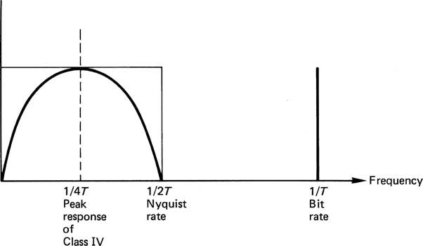
It has been stated that a magnetic head acts as a transversal filter, because it has two poles which scan the medium at different times. In addition the output is differentiated, so that the head may be thought of as a (1 min D) impulse response system, where D is the delay which is a function of the tape speed and gap size. It is this delay which results in intersymbol interference. Conventional equalizers attempt to oppose this effect, and succeed in raising the noise level in the process of making the frequency response linear. Figure 6.29 shows that the frequency response necessary to pass data with insignificant peak shift is a bandwidth of half the bit rate, which is the Nyquist rate. In Class IV partial response, the frequency response of the system is made to have nulls at DC and at the bit rate. Such a frequency response is particularly advantageous for rotary head recorders as it is DC-free and the low-frequency content is minimal, hence the use in Digital Betacam. The required response is achieved by an overall impulse response of (1–D²) where D is now the bit period. There are a number of ways in which this can be done.

Figure 6.29 Class IV response has spectral nulls at DC and the Nyquist rate, giving a noise advantage, since magnetic replay signal is weak at both frequencies in a high-density channel.

If the head gap is made equal to one bit, the (1–D) head response may be converted to the desired response by the use of a (1 + D) filter, as in Figure 6.30(a).9 Alternatively, a head of unspecified gapwidth may be connected to an integrator, and equalized flat to reproduce the record current waveform before being fed to a (1–D²) filter as in Figure 6.30(b).10

Figure 6.30 (a), (b) Two ways of obtaining partial response. (c) Characteristic eye pattern of ternary signal.

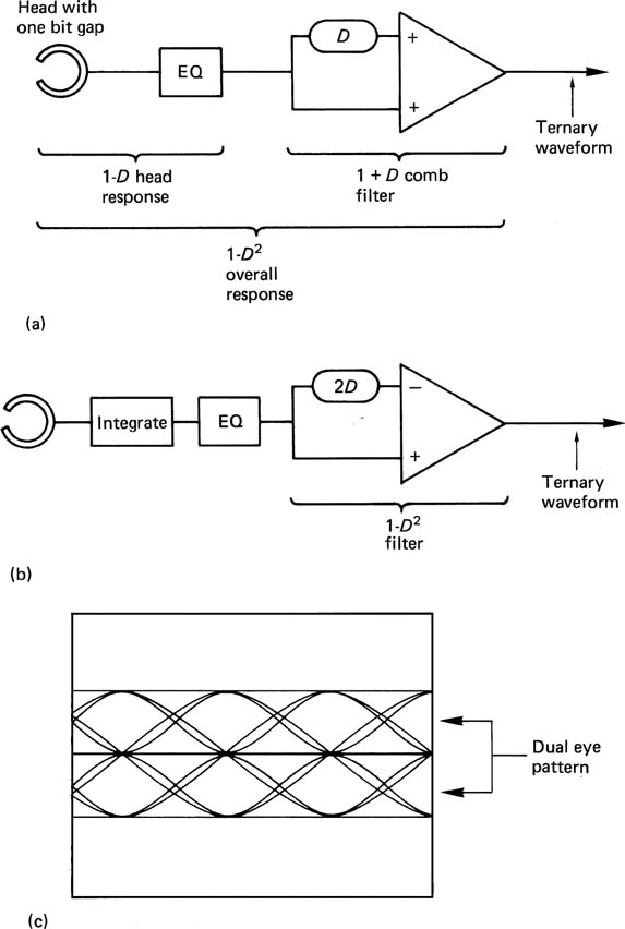
The result of both of these techniques is a ternary signal. The eye pattern has two sets of eyes as in Figure 6.30(c).11 When slicing such a signal, a smaller amount of noise will cause an error than in the binary case.

The treatment of the signal thus far represents an equalization technique, and not a channel code. However, to take full advantage of Class IV partial response, suitable precoding is necessary prior to recording, which does then constitute a channel-coding technique. This precoding is shown in Figure 6.31(a). Data are added modulo-2 to themselves with a two-bit delay. The effect of this precoding is that the outer levels of the ternary signals, which represent data ones, alternate in polarity on all odd bits and on all even bits. This is because the precoder acts like two interleaved one-bit delay circuits, as in Figure 6.31(b). As this alternation of polarity is a form of redundancy, it can be used to recover the 3 dB SNR loss encountered in slicing a ternary eye pattern (see Figure 6.32(a)).

Figure 6.31 Class IV precoding at (a) causes redundancy in replay signal as derived in (b).

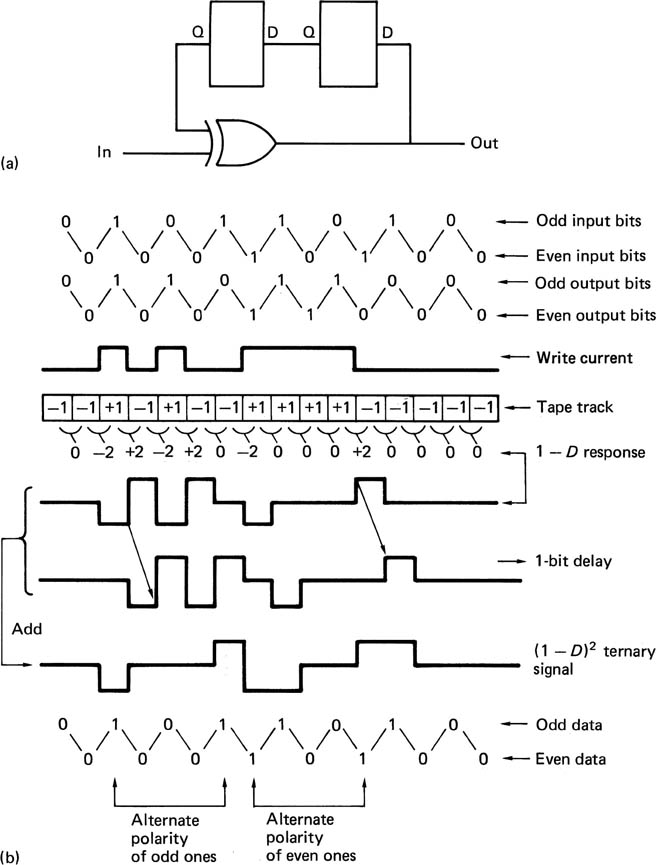
Figure 6.32 (a) A ternary signal suffers a noise penalty because there are two slicing levels. (b) The redundancy is used to determine the bit value in the presence of noise. Here the pulse height has been reduced to make it ambiguous 1/0, but only 1 is valid as zero violates the redundancy rules.

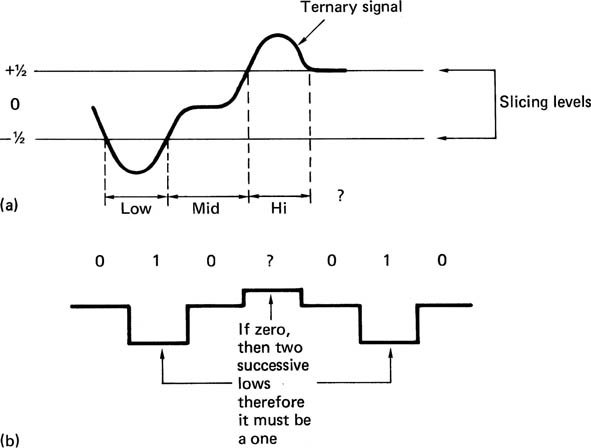
Viterbi decoding12 can be used for this purpose. In Viterbi decoding, each channel bit is not sliced individually; the slicing decision is made in the context of adjacent decisions. Figure 6.32(b) shows a replay waveform which is so noisy that, at the decision point, the signal voltage crosses the centre of the eye, and the slicer alone cannot tell whether the correct decision is an inner or an outer level. In this case, the decoder essentially allows both decisions to stand, in order to see what happens. A symbol representing indecision is output. It will be seen from the figure that as subsequent bits are received, one of these decisions will result in an absurd situation, which indicates that the other decision was the right one. The decoder can then locate the undecided symbol and set it to the correct value.

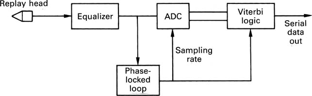
Viterbi decoding requires more information about the signal voltage than a simple binary slicer can discern. Figure 6.33 shows that the replay waveform is sampled and quantized so that it can be processed in digital logic. The sampling rate is obtained from the embedded clock content of the replay waveform. The digital Viterbi processing logic must be able to operate at high speed to handle serial signals from a DVTR head. Its application in Digital Betacam is eased somewhat by the adoption of compression which reduces the data rate at the heads by a factor of two.

Figure 6.33 A Viterbi decoder is implemented in the digital domain by sampling the replay waveform with a clock locked to the embedded clock of the channel code.

Clearly a ternary signal having a dual eye pattern is more sensitive than a binary signal, and it is important to keep the maximum run length T_max small in order to have accurate AGC. The use of pseudo-random coding along with partial response equalization and precoding is a logical combination.13

There is then considerable overlap between the channel code and the error-correction system. Viterbi decoding is primarily applicable to channels with random errors due to Gaussian statistics, and they cannot cope with burst errors. In a head-noise-limited system, however, the use of a Viterbi detector could increase the power of an separate burst error-correction system by relieving it of the need to correct random errors due to noise. The error-correction system could then concentrate on correcting burst errors unimpaired.

6.15 Synchronizing

Once the PLL in the data separator has locked to the clock content of the transmission, a serial channel bitstream and a channel bit clock will emerge from the sampler. In a group code, it is essential to know where a group of channel bits begins in order to assemble groups for decoding to data bit groups. In a randomizing system it is equally vital to know at what point in the serial data stream the words or samples commence. In serial transmission and in recording, channel bit groups or randomized data words are sent one after the other, one bit at a time, with no spaces in between, so that although the designer knows that a data block contains, say, 128 bytes, the receiver simply finds 1024 bits in a row. If the exact position of the first bit is not known, then it is not possible to put all the bits in the right places in the right bytes; a process known as deserializing. The effect of sync slippage is devastating, because a one-bit disparity between the bit count and the bitstream will corrupt every symbol in the block.

The synchronization of the data separator and the synchronization to the block format are two distinct problems, which are often solved by the same sync pattern. Deserializing requires a shift register which is fed with serial data and read out once per word. The sync detector is simply a set of logic gates which are arranged to recognize a specific pattern in the register. The sync pattern is either identical for every block or has a restricted number of versions and it will be recognized by the replay circuitry and used to reset the bit count through the block. Then by counting channel bits and dividing by the group size, groups can be deserialized and decoded to data groups. In a randomized system, the pseudorandom sequence generator is also reset. Then counting derandomized bits from the sync pattern and dividing by the wordlength enables the replay circuitry to deserialize the data words.

Even if a specific code were excluded from the recorded data so that it could be used for synchronizing, this cannot ensure that the same pattern cannot be falsely created at the junction between two allowable data words. Figure 6.34 shows how false synchronizing can occur due to concatenation. It is thus not practical to use a bit pattern which is a data code value in a simple synchronizing recognizer. The problem is overcome in some synchronous systems by using the fact that sync patterns occur exactly once per block and therefore contain redundancy. If the pattern is seen by the recognizer at block rate, a genuine sync condition exists. Sync patterns seen at other times must be false. Such systems take a few milliseconds before sync is achieved, but once achieved it should not be lost unless the transmission is interrupted.

Figure 6.34 Concatenation of two words can result in the accidental generation of a word which is reserved for synchronizing.

In run-length-limited codes false syncs are not a problem. The sync pattern is no longer a data bit pattern but is a specific waveform. If the sync waveform contains run lengths which violate the normal coding limits, there is no way that these run lengths can occur in encoded data, nor any possibility that they will be interpreted as data. They can, however, be readily detected by the replay circuitry.

In a group code there are many more combinations of channel bits than there are combinations of data bits. Thus after all data bit patterns have been allocated group patterns, there are still many unused group patterns which cannot occur in the data. With care, group patterns can be found which cannot occur due to the concatenation of any pair of groups representing data. These are then unique and can be used for synchronizing.

6.16 Basic error correction

There are many different types of recording and transmission channel and consequently there will be many different mechanisms which may result in errors. Bit errors in video cause ‘sparkles’ in the picture whose effect depends upon the significance of the affected bit. Errors in compressed data are more serious as they may cause the decoder to lose sync.

In magnetic recording, data can be corrupted by mechanical problems such as media dropout and poor tracking or head contact, or Gaussian thermal noise in replay circuits and heads. In optical recording, contamination of the medium interrupts the light beam. When group codes are used, a single defect in a group changes the group symbol and may cause errors up to the size of the group. Single-bit errors are therefore less common in group-coded channels. Inside equipment, data are conveyed on short wires and the noise environment is under the designer’s control. With suitable design techniques, errors can be made effectively negligible whereas in communication systems, there is considerably less control of the electromagnetic environment.

Irrespective of the cause, all these mechanisms cause one of two effects. There are large isolated corruptions, called error bursts, where numerous bits are corrupted all together in an area which is otherwise error-free, and there are random errors affecting single bits or symbols. Whatever the mechanism, the result will be that the received data will not be exactly the same as those sent. In binary the discrete bits will be each either right or wrong. If a binary digit is known to be wrong, it is only necessary to invert its state and then it must be right. Thus error correction itself is trivial; the hard part is working out which bits need correcting.

There are a number of terms which have idiomatic meanings in error correction. The raw BER (bit error rate) is the error rate of the medium, whereas the residual or uncorrected BER is the rate at which the error-correction system fails to detect or miscorrects errors. In practical digital systems, the residual BER is negligibly small. If the error correction is turned off, the two figures become the same.

Error correction works by adding some bits to the data which are calculated from the data. This creates an entity called a codeword which spans a greater length of time than one bit alone. The statistics of noise means that whilst one bit may be lost in a codeword, the loss of the rest of the codeword because of noise is highly improbable. As will be described later in this chapter, codewords are designed to be able to correct totally a finite number of corrupted bits. The greater the timespan over which the coding is performed, or, on a recording medium, the greater area over which the coding is performed, the greater will be the reliability achieved, although this does mean that an encoding delay will be experienced on recording, and a similar or greater decoding delay on reproduction.

Shannon14 disclosed that a message can be sent to any desired degree of accuracy provided that it is spread over a sufficient timespan. Engineers have to compromise, because an infinite coding delay in the recovery of an error-free signal is not acceptable. Digital interfaces such as SDI (see Chapter 9) do not employ error correction because the build-up of coding delays in large production systems is unacceptable.

If error correction is necessary as a practical matter, it is then only a small step to put it to maximum use. All error correction depends on adding bits to the original message, and this, of course, increases the number of bits to be recorded, although it does not increase the information recorded. It might be imagined that error correction is going to reduce storage capacity, because space has to be found for all the extra bits. Nothing could be further from the truth. Once an error-correction system is used, the signal-to-noise ratio of the channel can be reduced, because the raised BER of the channel will be overcome by the error-correction system. Reduction of the SNR by 3 dB in a magnetic track can be achieved by halving the track width, provided that the system is not dominated by head or preamplifier noise. This doubles the recording density, making the storage of the additional bits needed for error correction a trivial matter. By a similar argument, the power of a digital transmitter can be reduced if error correction is used. In short, error correction is not a nuisance to be tolerated; it is a vital tool needed to maximize the efficiency of storage devices and transmission. Convergent systems would not be economically viable without it.

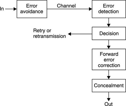
Figure 6.35 shows the broad subdivisions of error handling. The first stage might be called error avoidance and includes such measures as creating bad block files on hard disks or using verified media. Properly terminating network cabling is also in this category. Placing the audio blocks near to the centre of the tape in DVTRs is a further example. The data pass through the channel, which causes whatever corruptions it feels like. On receipt of the data the occurrence of errors is first detected, and this process must be extremely reliable, as it does not matter how effective the correction or how good the concealment algorithm, if it is not known that they are necessary! The detection of an error then results in a course of action being decided.

Figure 6.35 Error-handling strategies can be divided into avoiding errors, detecting errors and deciding what to do about them. Some possibilities are shown here. Of all these the detection is the most critical, as nothing can be done if the error is not detected.

In the case of a file transfer, real-time operation is not required. If a disk drive detects a read error a retry is easy as the disk is turning at several thousand rpm and will quickly re-present the data. An error due to a dust particle may not occur on the next revolution. A packet in error in a network will result in a retransmission. Many magnetic tape systems have read after write. During recording, offtape data are immediately checked for errors. If an error is detected, the tape may abort the recording, reverse to the beginning of the current block and erase it. The data from that block may then be recorded further down the tape. This is the recording equivalent of a retransmission in a communications system.

In many cases of digital video or audio replay a retry or retransmission is not possible because the data are required in real time. In this case the solution is to encode the message using a system which is sufficiently powerful to correct the errors in real time. These are called forward error-correcting schemes (FEC). The term ‘forward’ implies that the transmitter does not need to take any action in the case of an error; the receiver will perform the correction.

6.17 Concealment by interpolation

There are some practical differences between data recording for video and the computer data recording application. Although video or audio recorders seldom have time for retries, they have the advantage that there is a certain amount of redundancy in the information conveyed. Thus if an error cannot be corrected, then it can be concealed. If a sample is lost, it is possible to obtain an approximation to it by interpolating between samples in the vicinity of the missing one. Clearly, concealment of any kind cannot be used with computer instructions or compressed data, although concealment can be applied after compressed signals have been decoded.

If there is too much corruption for concealment, the only course in video is repeat the previous field or frame in a freeze as it is unlikely that the corrupt picture is watchable. In audio the equivalent is muting.

In general, if use is to be made of concealment on replay, the data must generally be reordered or shuffled prior to recording. To take a simple example, odd-numbered samples are recorded in a different area of the medium from even-numbered samples. On playback, if a gross error occurs on the medium, depending on its position, the result will be either corrupted odd samples or corrupted even samples, but it is most unlikely that both will be lost. Interpolation is then possible if the power of the correction system is exceeded. In practice the shuffle employed in digital video recorders is two-dimensional and rather more complex. Further details can be found in Chapter 8. The concealment technique described here is only suitable for PCM recording. If compression has been employed, different concealment techniques will be needed.

It should be stressed that corrected data are undistinguishable from the original and thus there can be no visible or audible artifacts. In contrast, concealment is only an approximation to the original information and could be detectable. In practical equipment, concealment occurs infrequently unless there is a defect requiring attention, and its presence is difficult to see.

6.18 Parity

The error-detection and error-correction processes are closely related and will be dealt with together here. The actual correction of an error is simplified tremendously by the adoption of binary. As there are only two symbols, 0 and 1, it is enough to know that a symbol is wrong, and the correct value is obvious. Figure 6.36 shows a minimal circuit required for correction once the bit in error has been identified. The XOR (exclusive-OR) gate shows up extensively in error correction and the figure also shows the truth table. One way of remembering the characteristics of this useful device is that there will be an output when the inputs are different. Inspection of the truth table will show that there is an even number of ones in each row (zero is an even number) and so the device could also be called an even parity gate. The XOR gate is also a adder in modulo-2.

Figure 6.36 Once the position of the error is identified, the correction process in binary is easy.

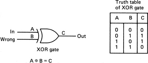
Parity is a fundamental concept in error detection. In Figure 6.37, the example is given of a four-bit data word which is to be protected. If an extra bit is added to the word which is calculated in such a way that the total number of ones in the five-bit word is even, this property can be tested on receipt. The generation of the parity bit can be performed by a number of the ubiquitous XOR gates configured into what is known as a parity tree. In the figure, if a bit is corrupted, the received message will be seen no longer to have an even number of ones. If two bits are corrupted, the failure will be undetected. This example can be used to introduce much of the terminology of error correction. The extra bit added to the message carries no information of its own, since it is calculated from the other bits. It is therefore called a redundant bit.

Figure 6.37 Parity checking adds up the number of ones in a word using, in this example, parity trees. One error bit and odd numbers of errors are detected. Even numbers of errors cannot be detected.

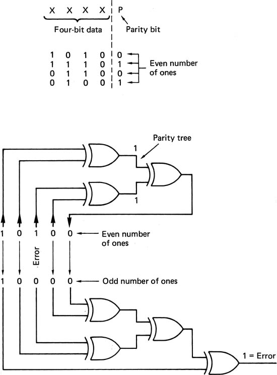
The addition of the redundant bit gives the message a special property, i.e. the number of ones is even. A message having some special property irrespective of the actual data content is called a codeword. All error correction relies on adding redundancy to real data to form codewords for transmission. If any corruption occurs, the intention is that the received message will not have the special property; in other words, if the received message is not a codeword there has definitely been an error. The receiver can check for the special property without any prior knowledge of the data content. Thus the same check can be made on all received data. If the received message is a codeword, there probably has not been an error. The word ‘probably’ must be used because the figure shows that two bits in error will cause the received message to be a codeword, which cannot be discerned from an error-free message.

If it is known that generally the only failure mechanism in the channel in question is loss of a single bit, it is assumed that receipt of a codeword means that there has been no error. If there is a probability of two error bits, that becomes very nearly the probability of failing to detect an error, since all odd numbers of errors will be detected, and a four-bit error is much less likely. It is paramount in all error-correction systems that the protection used should be appropriate for the probability of errors to be encountered. An inadequate error-correction system is actually worse than not having any correction. Error correction works by trading probabilities. Error-free performance with a certain error rate is achieved at the expense of performance at higher error rates. Figure 6.38 shows the effect of an error-correction system on the residual BER for a given raw BER. It will be seen that there is a characteristic knee in the graph. If the expected raw BER has been misjudged, the consequences can be disastrous. Another result demonstrated by the example is that we can only guarantee to detect the same number of bits in error as there are redundant bits.

Figure 6.38 An error-correction system can only reduce errors at normal error rates at the expense of increasing errors at higher rates. It is most important to keep a system working to the left of the knee in the graph.

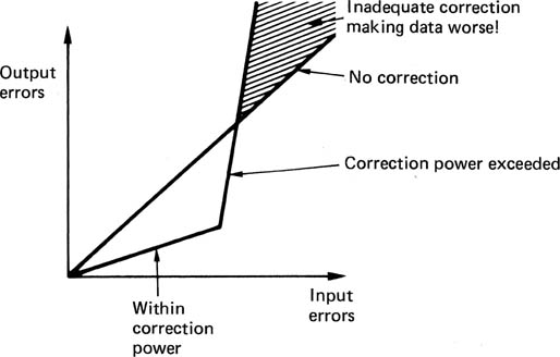
6.19 Block and convolutional codes

Figure 6.39(a) shows a strategy known as a crossword code, or product code. The data are formed into a two-dimensional array, in which each location can be a single bit or a multi-bit symbol. Parity is then generated on both rows and columns. If a single bit or symbol fails, one row parity check and one column parity check will fail, and the failure can be located at the intersection of the two failing checks. Although two symbols in error confuse this simple scheme, using more complex coding in a two-dimensional structure is very powerful, and further examples will be given throughout this chapter.

Figure 6.39 A block code is shown in (a). Each location in the block can be a bit or a word. Horizontal parity checks are made by adding P1, P2, etc., and cross-parity or vertical checks are made by adding CP1, CP2, etc. Any symbol in error will be at the intersection of the two failing codewords.

In (b) a convolutional coder is shown. Symbols entering are subject to different delays which result in the codewords in (c) being calculated. These have a vertical part and a diagonal part. A symbol in error will be at the intersection of the diagonal part of one code and the vertical part of another.

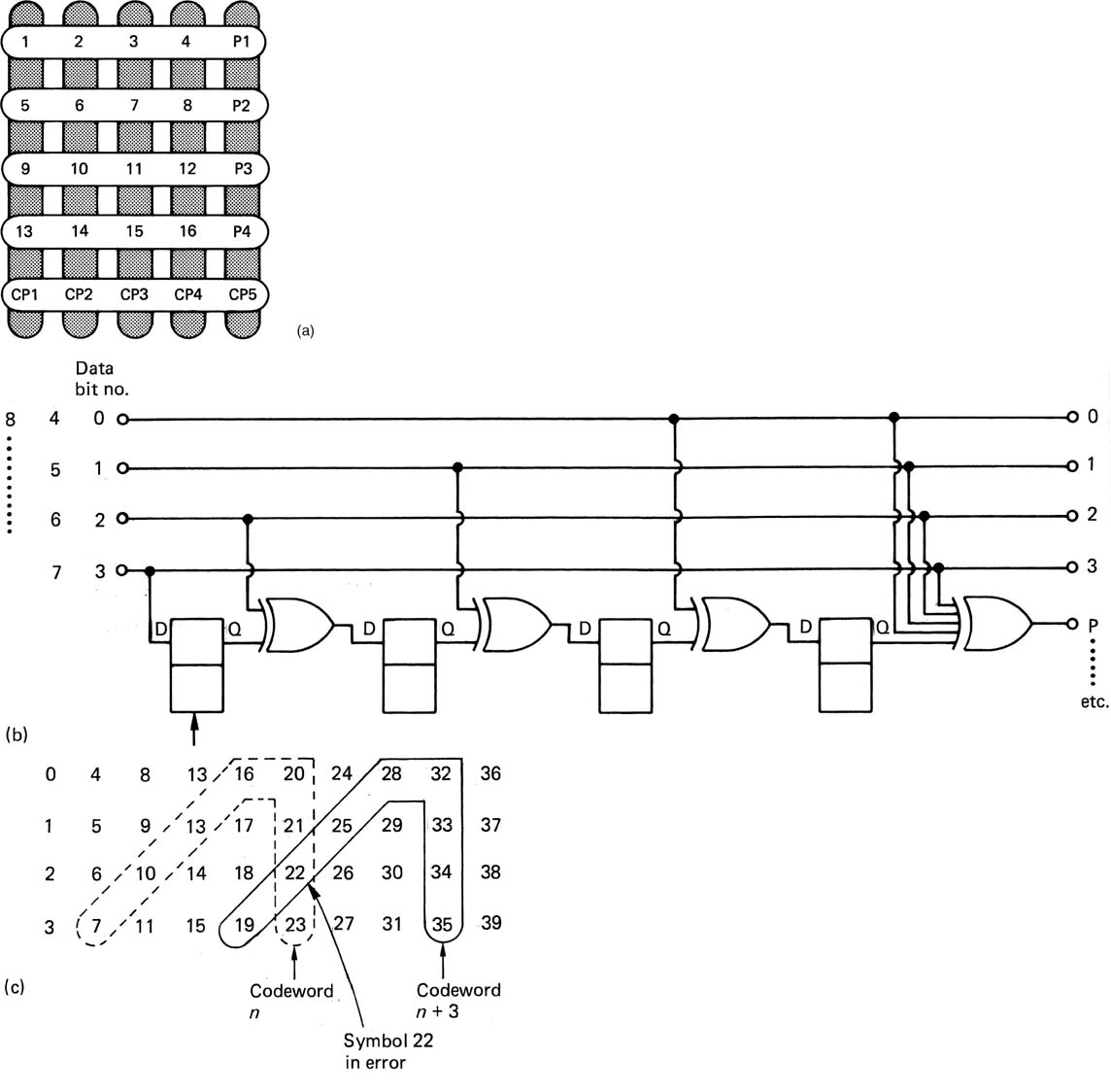
The example of Figure 6.39(a) assembles the data to be coded into a block of finite size and then each codeword is calculated by taking a different set of symbols. This should be contrasted with the operation of the circuit of Figure 6.39(b). Here the data are not in a block, but form an endless stream. A shift register allows four symbols to be available simultaneously to the encoder. The action of the encoder depends upon the delays. When symbol 3 emerges from the first delay, it will be added (modulo-2) to symbol 6. When this sum emerges from the second delay, it will be added to symbol 9 and so on. The codeword produced is shown in Figure 6.39(c) where it will be seen to be bent such that it has a vertical section and a diagonal section. Four symbols later the next codeword will be created one column further over in the data.

This is a convolutional code because the coder always takes parity on the same pattern of symbols which is convolved with the data stream on an endless basis. Figure 6.39(c) also shows that if an error occurs, it can be located because it will cause parity errors in two codewords. The error will be on the diagonal part of one codeword and on the vertical part of the other so that it can be located uniquely at the intersection and corrected by parity.

Comparison with the block code of Figure 6.39(a) will show that the convolutional code needs less redundancy for the same single-symbol location and correction performance as only a single redundant symbol is required for every four data symbols. Convolutional codes are computed on an endless basis which makes them inconvenient in recording applications where editing is anticipated. Here the block code is more appropriate as it allows edit gaps to be created between codes. In the case of uncorrectable errors, the convolutional principle causes the syndromes to be affected for some time afterwards and results in miscorrections of symbols which were not actually in error. This is called error propagation and is a characteristic of convolutional codes. Recording media tend to produce somewhat variant error statistics because media defects and mechanical problems cause errors which do not fit the classical additive noise channel. Convolutional codes can easily be taken beyond their correcting power if used with real recording media.

In transmission and broadcasting, the error statistics are more stable and the editing requirement is absent. As a result, convolutional codes tend to be used in digital broadcasting as will be seen in Chapter 9.

6.20 Cyclic codes

In digital recording applications, the data are stored serially on a track, and it is desirable to use relatively large data blocks to reduce the amount of the medium devoted to preambles, addressing and synchronizing. The principle of codewords having a special characteristic will still be employed, but they will be generated and checked algorithmically by equations. The syndrome will then be converted to the bit(s) in error by solving equations.

Where data can be accessed serially, simple circuitry can be used because the same gate will be used for many XOR operations. The circuit of Figure 6.40 is a kind of shift register, but with a particular feedback arrangement which leads it to be known as a twisted-ring counter. If seven message bits A-G are applied serially to this circuit, and each one of them is clocked, the outcome can be followed in the diagram. As bit A is presented and the system is clocked, bit A will enter the left-hand latch. When bits B and C are presented, A moves across to the right. Both XOR gates will have A on the upper input from the right-hand latch, the left one has D on the lower input and the right one has B on the lower input. When clocked, the left latch will thus be loaded with the XOR of A and D, and the right one with the XOR of A and B. The remainder of the sequence can be followed, bearing in mind that when the same term appears on both inputs of an XOR gate, it goes out, as the exclusive-OR of something with itself is nothing. At the end of the process, the latches contain three different expressions.

Figure 6.40 When seven successive bits A-G are clocked into this circuit, the contents of the three latches are shown for each clock. The final result is a parity-check matrix.

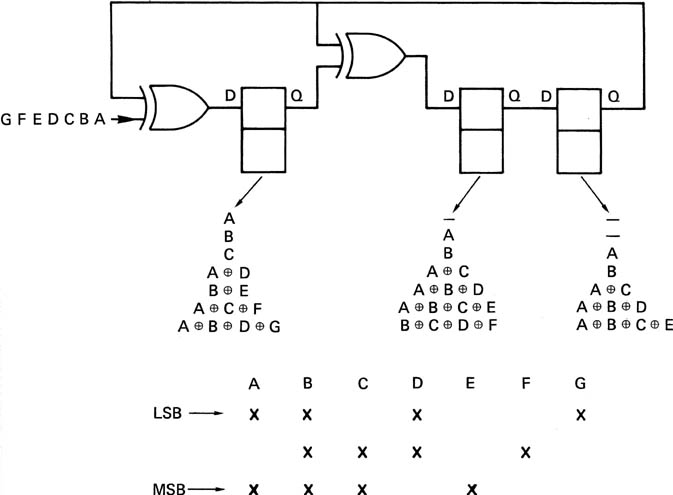
Essentially, the circuit makes three parity checks through the message, leaving the result of each in the three stages of the register. In the figure, these expressions have been used to draw up a check matrix. The significance of these steps can now be explained.

The bits ABC and D are four data bits, and the bits E F and G are redundancy. When the redundancy is calculated, bit E is chosen so that there are an even number of ones in bits A B C and E; bit F is chosen such that the same applies to bits B C D and F, and similarly for bit G. Thus the four data bits and the three check bits form a seven-bit codeword. If there is no error in the codeword, when it is fed into the circuit shown, the result of each of the three parity checks will be zero and every stage of the shift register will be cleared. As the register has eight possible states, and one of them is the error-free condition, then there are seven remaining states, hence the seven-bit codeword. If a bit in the codeword is corrupted, there will be a non-zero result. For example, if bit D fails, the check on bits A B D and G will fail, and a one will appear in the left-hand latch. The check on bits B C D F will also fail, and the centre latch will set. The check on bits A B C E will not fail, because D is not involved in it, making the right-hand bit zero. There will be a syndrome of 110 in the register, and this will be seen from the check matrix to correspond to an error in bit D. Whichever bit fails, there will be a different three-bit syndrome which uniquely identifies the failed bit. As there are only three latches, there can be eight different syndromes. One of these is zero, which is the error-free condition, and so there are seven remaining error syndromes. The length of the codeword cannot exceed seven bits, or there would not be enough syndromes to correct all the bits. This can also be made to tie in with the generation of the check matrix. If fourteen bits, A to N, were fed into the circuit shown, the result would be that the check matrix repeated twice, and if a syndrome of 101 were to result, it could not be determined whether bit D or bit K failed. Because the check repeats every seven bits, the code is said to be a cyclic redundancy check (CRC) code.

It has been seen that the circuit shown makes a matrix check on a received word to determine if there has been an error, but the same circuit can also be used to generate the check bits. To visualize how this is done, examine what happens if only the data bits A B C and D are known, and the check bits E F and G are set to zero. If this message, ABCD000, is fed into the circuit, the left-hand latch will afterwards contain the XOR of ABC and zero, which is, of course, what E should be. The centre latch will contain the XOR of BCD and zero, which is what F should be and so on. This process is not quite ideal, however, because it is necessary to wait for three clock periods after entering the data before the check bits are available. Where the data are simultaneously being recorded and fed into the encoder, the delay would prevent the check bits being easily added to the end of the data stream. This problem can be overcome by slightly modifying the encoder circuit as shown in Figure 6.41. By moving the position of the input to the right, the operation of the circuit is advanced so that the check bits are ready after only four clocks. The process can be followed in the diagram for the four data bits A B C and D. On the first clock, bit A enters the left two latches, whereas on the second clock, bit B will appear on the upper input of the left XOR gate, with bit A on the lower input, causing the centre latch to load the XOR of A and B and so on.

Figure 6.41 By moving the insertion point three places to the right, the calculation of the check bits is completed in only four clock periods and they can follow the data immediately. This is equivalent to premultiplying the data by x³.

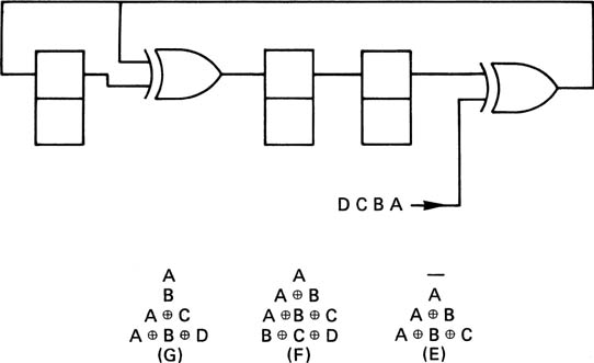
The way in which the cyclic codes work has been described in engineering terms, but it can be described mathematically if analysis is contemplated.

Just as the position of a decimal digit in a number determines the power of ten (whether that digit means one, ten or a hundred), the position of a binary digit determines the power of two (whether it means one, two or four). It is possible to rewrite a binary number so that it is expressed as a list of powers of two. For example, the binary number 1101 means 8 + 4 + 1, and can be written:

In fact, much of the theory of error correction applies to symbols in number bases other than 2, so that the number can also be written more generally as

which also looks much more impressive. This expression, containing as it does various powers, is, of course, a polynomial, and the circuit of Figure 6.40 which has been seen to construct a parity-check matrix on a codeword can also be described as calculating the remainder due to dividing the input by a polynomial using modulo-2 arithmetic. In modulo-2 there are no borrows or carries, and addition and subtraction are replaced by the XOR function, which makes hardware implementation very easy. In Figure 6.42 it will be seen that the circuit of Figure 6.40 actually divides the codeword by a polynomial which is

Figure 6.42 Circuit of Figure 6.40 divides by x³ + x + 1 to find remainder. At (b) this is used to calculate check bits. At (c) right, zero syndrome, no error.

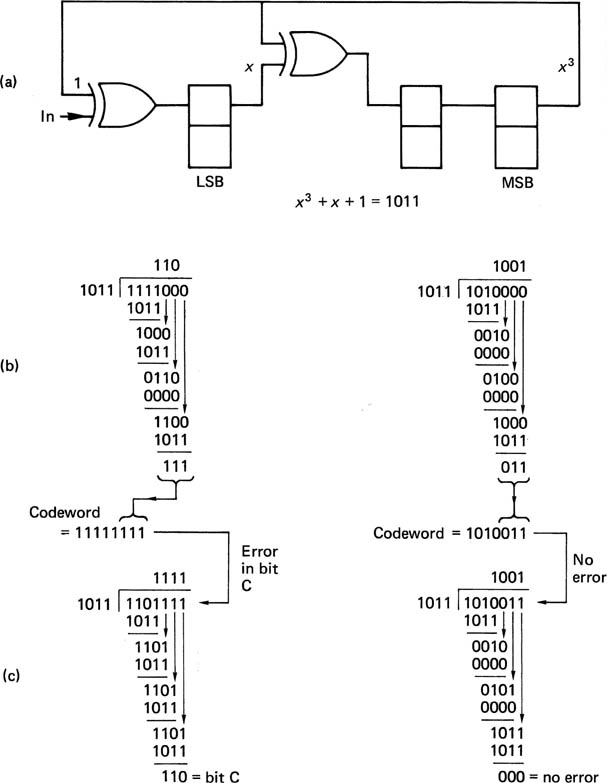
This can be deduced from the fact that the right-hand bit is fed into two lower-order stages of the register at once. Once all the bits of the message have been clocked in, the circuit contains the remainder. In mathematical terms, the special property of a codeword is that it is a polynomial which yields a remainder of zero when divided by the generating polynomial. The receiver will make this division, and the result should be zero in the error-free case. Thus the codeword itself disappears from the division. If an error has occurred it is considered that this is due to an error polynomial which has been added to the codeword polynomial. If a codeword divided by the check polynomial is zero, a non-zero syndrome must represent the error polynomial divided by the check polynomial. Thus if the syndrome is multiplied by the check polynomial, the latter will be cancelled out and the result will be the error polynomial. If this is added modulo-2 to the received word, it will cancel out the error and leave the corrected data.

Some examples of modulo-2 division are given in Figure 6.42 which can be compared with the parallel computation of parity checks according to the matrix of Figure 6.40.

The process of generating the codeword from the original data can also be described mathematically. If a codeword has to give zero remainder when divided, it follows that the data can be converted to a codeword by adding the remainder when the data are divided. Generally speaking, the remainder would have to be subtracted, but in modulo-2 there is no distinction. This process is also illustrated in Figure 6.42. The four data bits have three zeros placed on the righthand end, to make the wordlength equal to that of a codeword, and this word is then divided by the polynomial to calculate the remainder. The remainder is added to the zero-extended data to form a codeword. The modified circuit of Figure 6.41 can be described as premultiplying the data by x³ before dividing.

CRC codes are of primary importance for detecting errors, and several have been standardized for use in digital communications. The most common of these are:

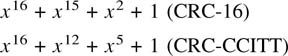
The sixteen-bit cyclic codes have codewords of length 2¹⁶−1 or 65 535 bits long. This may be too long for the application. Another problem with very long codes is that with a given raw BER, the longer the code, the more errors will occur in it. There may be enough errors to exceed the power of the code. The solution in both cases is to shorten or puncture the code. Figure 6.43 shows that in a punctured code, only the end of the codeword is used, and the data and redundancy are preceded by a string of zeros. It is not necessary to record these zeros, and, of course, errors cannot occur in them. Implementing a punctured code is easy. If a CRC generator starts with the register cleared and is fed with serial zeros, it will not change its state. Thus it is not necessary to provide the zeros, encoding can begin with the first data bit. In the same way, the leading zeros need not be provided during playback. The only precaution needed is that if a syndrome calculates the location of an error, this will be from the beginning of the codeword not from the beginning of the data. Where codes are used for detection only, this is of no consequence.

Figure 6.43 Codewords are often shortened, or punctured, which means that only the end of the codeword is actually transmitted. The only precaution to be taken when puncturing codes is that the computed position of an error will be from the beginning of the codeword, not from the beginning of the message.

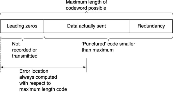
6.21 Introduction to the Reed-Solomon codes

The Reed-Solomon codes (Irving Reed and Gustave Solomon) are inherently burst correcting15 because they work on multi-bit symbols rather than individual bits. The R–S codes are also extremely flexible in use. One code may be used both to detect and correct errors and the number of bursts which are correctable can be chosen at the design stage by the amount of redundancy. A further advantage of the R–S codes is that they can be used in conjunction with a separate error-detection mechanism in which case they perform the correction only by erasure. R-S codes operate at the theoretical limit of correcting efficiency. In other words, no more efficient code can be found.

In the simple CRC system described in section 6.20, the effect of the error is detected by ensuring that the codeword can be divided by a polynomial. The CRC codeword was created by adding a redundant symbol to the data. In the Reed–Solomon codes, several errors can be isolated by ensuring that the codeword will divide by a number of polynomials. Clearly, if the codeword must divide by, say, two polynomials, it must have two redundant symbols. This is the minimum case of an R–S code. On receiving an R–S-coded message there will be two syndromes following the division. In the error-free case, these will both be zero. If both are not zero, there is an error.

It has been stated that the effect of an error is to add an error polynomial to the message polynomial. The number of terms in the error polynomial is the same as the number of errors in the codeword. The codeword divides to zero and the syndromes are a function of the error only. There are two syndromes and two equations. By solving these simultaneous equations it is possible to obtain two unknowns. One of these is the position of the error, known as the locator and the other is the error bit pattern, known as the corrector. As the locator is the same size as the code symbol, the length of the codeword is determined by the size of the symbol. A symbol size of eight bits is commonly used because it fits in conveniently with both sixteen-bit audio samples and byte-oriented computers. An eight-bit syndrome results in a locator of the same wordlength. Eight bits have 2⁸ combinations, but one of these is the error-free condition, and so the locator can specify one of only 255 symbols. As each symbol contains eight bits, the codeword will be 255 × 8 = 2040 bits long.

As further examples, five-bit symbols could be used to form a codeword 31 symbols long, and three-bit symbols would form a codeword seven symbols long. This latter size is small enough to permit some worked examples, and will be used further here. Figure 6.44 shows that in the seven-symbol codeword, five symbols of three bits each, A-E, are the data, and P and Q are the two redundant symbols. This simple example will locate and correct a single symbol in error. It does not matter, however, how many bits in the symbol are in error.

Figure 6.44 A Reed–Solomon codeword. As the symbols are of three bits, there can only be eight possible syndrome values. One of these is all zeros, the error-free case, and so it is only possible to point to seven errors: hence the codeword length of seven symbols. Two of these are redundant, leaving five data symbols.

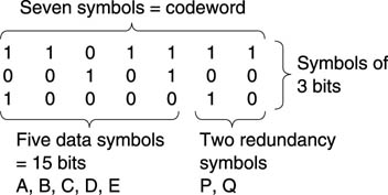
The two check symbols are solutions to the following equations:

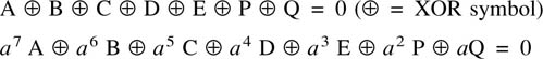
where a is a constant. The original data A-E followed by the redundancy P and Q pass through the channel.

The receiver makes two checks on the message to see if it is a codeword. This is done by calculating syndromes using the following expressions, where the (‘) implies the received symbol which is not necessarily correct:

(This is in fact a simple parity check.)

If two syndromes of all zeros are not obtained, there has been an error. The information carried in the syndromes will be used to correct the error. For the purpose of illustration, let it be considered that D’ has been corrupted before moving to the general case. D’ can be considered to be the result of adding an error of value E to the original value D such that D′ = D ⊕ E.

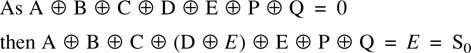
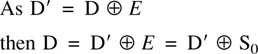
Thus the value of the corrector is known immediately because it is the same as the parity syndrome S0. The corrected data symbol is obtained simply by adding S0 to the incorrect symbol.

At this stage, however, the corrupted symbol has not yet been identified, but this is equally straightforward:

then:

Thus the syndrome S1 is the error bit pattern E, but it has been raised to a power of a which is a function of the position of the error symbol in the block. If the position of the error is in symbol k, then k is the locator value and:

Hence:

The value of k can be found by multiplying S0 by various powers of a until the product is the same as S1. Then the power of a necessary is equal to k. The use of the descending powers of a in the codeword calculation is now clear because the error is then multiplied by a different power of a dependent upon its position, known as the locator, because it gives the position of the error. The process of finding the error position by experiment is known as a Chien search.

Whilst the expressions above show that the values of P and Q are such that the two syndrome expressions sum to zero, it is not yet clear how P and Q are calculated from the data. Expressions for P and Q can be found by solving the two R–S equations simultaneously. This has been done in Appendix 6.1. The following expressions must be used to calculate P and Q from the data in order to satisfy the codeword equations. These are:

In both the calculation of the redundancy shown here and the calculation of the corrector and the locator it is necessary to perform numerous multiplications and raising to powers. This appears to present a formidable calculation problem at both the encoder and the decoder. This would be the case if the calculations involved were conventionally executed. However, the calculations can be simplified by using logarithms. Instead of multiplying two numbers, their logarithms are added. In order to find the cube of a number, its logarithm is added three times. Division is performed by subtracting the logarithms. Thus all the manipulations necessary can be achieved with addition or subtraction, which is straightforward in logic circuits.

The success of this approach depends upon simple implementation of log tables. As was seen in section 2.26, raising a constant, a, known as the primitive element to successively higher powers in modulo-2 gives rise to a Galois field. Each element of the field represents a different power n of a. It is a fundamental of the R–S codes that all the symbols used for data, redundancy and syndromes are considered to be elements of a Galois field. The number of bits in the symbol determines the size of the Galois field, and hence the number of symbols in the codeword.

In Figure 6.45, the binary values of the elements are shown alongside the power of a they represent. In the R–S codes, symbols are no longer considered simply as binary numbers, but also as equivalent powers of a. In Reed–Solomon coding and decoding, each symbol will be multiplied by some power of a. Thus if the symbol is also known as a power of a it is only necessary to add the two powers. For example, if it is necessary to multiply the data symbol 100 by a³, the calculation proceeds as follows, referring to Figure 6.45.

Figure 6.45 The bit patterns of a Galois field expressed as powers of the primitive element a. This diagram can be used as a form of log table in order to multiply binary numbers. Instead of an actual multiplication, the appropriate powers of a are simply added.

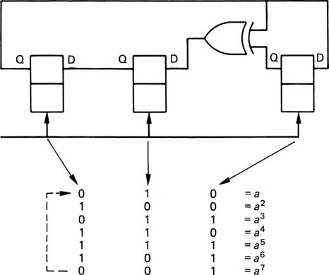
Note that the results of a Galois multiplication are quite different from binary multiplication. Because all products must be elements of the field, sums of powers which exceed seven wrap around by having seven subtracted. For example:

Figure 6.46 shows some examples of circuits which will perform this kind of multiplication. Note that they require a minimum amount of logic.

Figure 6.46 Some examples of GF multiplier circuits.

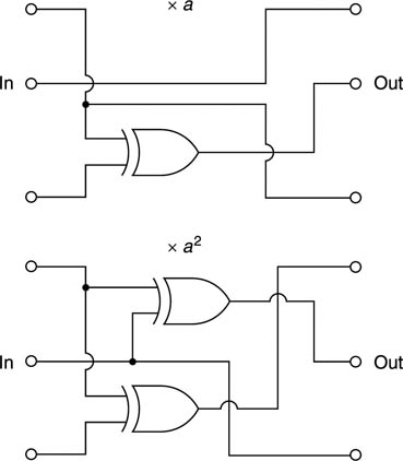
Figure 6.47 given an example of the Reed–Solomon encoding process. The Galois field shown in Figure 6.45 has been used, having the primitive element a = 010. At the beginning of the calculation of P, the symbol A is multiplied by a⁶. This is done by converting A to a power of a. According to Figure 6.45, 101 = a⁶ and so the product will be a^{(6 + 6)} = a¹² = a⁵ = 111. In the same way, B is multiplied by a, and so on, and the products are added modulo-2. A similar process is used to calculate Q.

Figure 6.47 Five data symbols A-E are used as terms in the generator polynomials derived in Appendix 6.1 to calculate two redundant symbols P and Q. An example is shown at the top. Below is the result of using the codeword symbols A-Q as terms in the checking polynomials. As there is no error, both syndromes are zero.

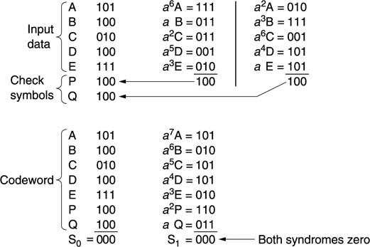
Figure 6.48 shows a circuit which can calculate P or Q. The symbols A-E are presented in succession, and the circuit is clocked for each one. On the first clock, a⁶ A is stored in the left-hand latch. If B is now provided at the input, the second GF multiplier produces aB and this is added to the output of the first latch and when clocked will be stored in the second latch which now contains a⁶ A + aB. The process continues in this fashion until the complete expression for P is available in the right-hand latch. The intermediate contents of the right-hand latch are ignored.

Figure 6.48 If the five data symbols of Figure 6.47 are supplied to this circuit in sequence, after five clocks, one of the check symbols will appear at the output. Terms without brackets will calculate P, bracketed terms calculate Q.

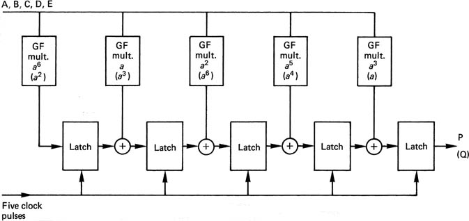
The entire codeword now exists, and can be recorded or transmitted. Figure 6.47 also demonstrates that the codeword satisfies the checking equations. The modulo-2 sum of the seven symbols, S₀, is 000 because each column has an even number of ones. The calculation of S₁ requires multiplication by descending powers of a. The modulo-2 sum of the products is again zero. These calculations confirm that the redundancy calculation was properly carried out.

Figure 6.49 gives three examples of error correction based on this codeword. The erroneous symbol is marked with a dash. As there has been an error, the syndromes S₀ and S₁ will not be zero.

Figure 6.49 Three examples of error location and correction. The number of bits in error in a symbol is irrelevant; if all three were wrong, S₀ would be 111, but correction is still possible.

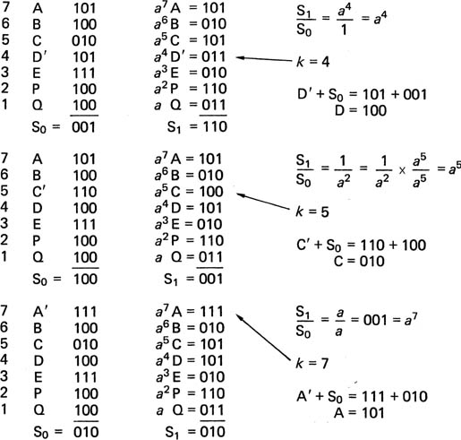
Figure 6.50 shows circuits suitable for parallel calculation of the two syndromes at the receiver. The S0 circuit is a simple parity checker which accumulates the modulo-2 sum of all symbols fed to it. The S₁ circuit is more subtle, because it contains a Galois field (GF) multiplier in a feedback loop, such that early symbols fed in are raised to higher powers than later symbols because they have been recirculated through the GF multiplier more often. It is possible to compare the operation of these circuits with the example of Figure 6.49 and with subsequent examples to confirm that the same results are obtained.

Figure 6.50 Circuits for parallel calculation of syndromes S₀, S₁, S₀ is a simple parity check. S₁ has a GF multiplication by a in the feedback, so that A is multiplied by a⁷, B is multiplied by a⁶, etc., and all are summed to give S₁.

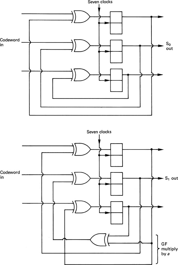
6.22 Correction by erasure

In the examples of Figure 6.49, two redundant symbols P and Q have been used to locate and correct one error symbol. If the positions of errors are known by some separate mechanism (see product codes, section 6.24) the locator need not be calculated. The simultaneous equations may instead be solved for two correctors. In this case the number of symbols which can be corrected is equal to the number of redundant symbols. In Figure 6.51(a) two errors have taken place, and it is known that they are in symbols C and D. Since S0 is a simple parity check, it will reflect the modulo-2 sum of the two errors. Hence S₁ = EC ⊕ ED.

Figure 6.51 If the location of errors is known, then the syndromes are a known function of the two errors as shown in (a). It is, however, much simpler to set the incorrect symbols to zero, i.e. to erase them as in (b). Then the syndromes are a function of the wanted symbols and correction is easier.

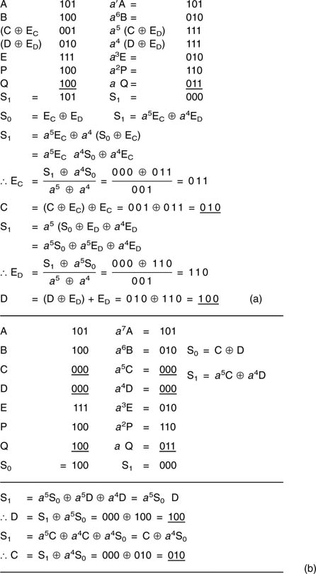
The two errors will have been multiplied by different powers in S1, such that:

These two equations can be solved, as shown in the figure, to find EC and ED, and the correct value of the symbols will be obtained by adding these correctors to the erroneous values. It is, however, easier to set the values of the symbols in error to zero. In this way the nature of the error is rendered irrelevant and it does not enter the calculation. This setting of symbols to zero gives rise to the term erasure. In this case,

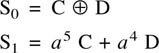
Erasing the symbols in error makes the errors equal to the correct symbol values and these are found more simply as shown in Figure 6.51(b)

Practical systems will be designed to correct more symbols in error than in the simple examples given here. If it is proposed to correct by erasure an arbitrary number of symbols in error given by t, the codeword must be divisible by t different polynomials. Alternatively, if the errors must be located and corrected, 2t polynomials will be needed. These will be of the form (x + aⁿ) where n takes all values up to t or 2t. a is the primitive element discussed in section 2.26.

Where four symbols are to be corrected by erasure, or two symbols are to be located and corrected, four redundant symbols are necessary, and the codeword polynomial must then be divisible by

Upon receipt of the message, four syndromes must be calculated, and the four correctors or the two error patterns and their positions are determined by solving four simultaneous equations. This generally requires an iterative procedure, and a number of algorithms have been developed for the purpose.16–18 Modern DVTR formats use eight-bit R–S codes and erasure extensively. The primitive polynomial commonly used with GF(256) is:

The codeword will be 255 bytes long but will often be shortened by puncturing. The larger Galois fields require less redundancy, but the computational problem increases. LSI chips have been developed specifically for R–S decoding in many high-volume formats.

6.23 Interleaving

The concept of bit interleaving was introduced in connection with a single-bit correcting code to allow it to correct small bursts. With burst-correcting codes such as Reed-Solomon, bit interleave is unnecessary. In most channels, particularly high-density recording channels used for digital video or audio, the burst size may be many bytes rather than bits, and to rely on a code alone to correct such errors would require a lot of redundancy. The solution in this case is to employ symbol interleaving, as shown in Figure 6.52. Several codewords are encoded from input data, but these are not recorded in the order they were input, but are physically reordered in the channel, so that a real burst error is split into smaller bursts in several codewords. The size of the burst seen by each codeword is now determined primarily by the parameters of the interleave, and Figure 6.53 shows that the probability of occurrence of bursts with respect to the burst length in a given codeword is modified. The number of bits in the interleave word can be made equal to the burst-correcting ability of the code in the knowledge that it will be exceeded only very infrequently.

Figure 6.52 The interleave controls the size of burst errors in individual codewords.

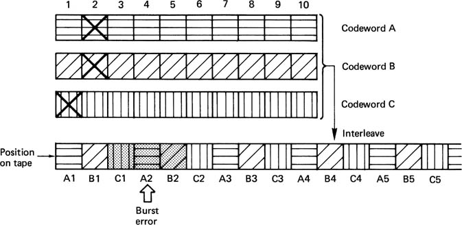
Figure 6.53 (a) The distribution of burst sizes might look like this. (b) Following interleave, the burst size within a codeword is controlled to that of the interleave symbol size, except for gross errors which have low probability.

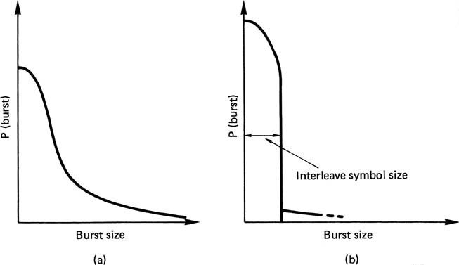
There are a number of different ways in which interleaving can be performed. Figure 6.54 shows that in block interleaving, words are reordered within blocks which are themselves in the correct order. This approach is attractive for rotary-head recorders, because the scanning process naturally divides the tape up into blocks. The block interleave is achieved by writing samples into a memory in sequential address locations from a counter, and reading the memory with non-sequential addresses from a sequencer. The effect is to convert a one-dimensional sequence of samples into a two-dimensional structure having rows and columns.

Figure 6.54 In block interleaving, data are scrambled within blocks which are themselves in the correct order.

The alternative to block interleaving is convolutional interleaving where the interleave process is endless. In Figure 6.55 symbols are assembled into short blocks and then delayed by an amount proportional to the position in the block. It will be seen from the figure that the delays have the effect of shearing the symbols so that columns on the left side of the diagram become diagonals on the right. When the columns on the right are read, the convolutional interleave will be obtained. Convolutional interleave works well in transmission applications such as DVB where there is no natural track break. Convolutional interleave has the advantage of requiring less memory to implement than a block code. This is because a block code requires the entire block to be written into the memory before it can be read, whereas a convolutional code requires only enough memory to cause the required delays.

Figure 6.55 In convolutional interleaving, samples are formed into a rectangular array, which is sheared by subjecting each row to a different delay. The sheared array is read in vertical columns to provide the interleaved output. In this example, samples will be found at 4, 8 and 12 places away from their original order.

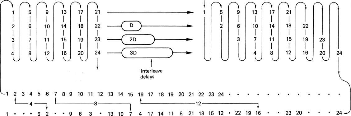
6.24 Product codes

In the presence of burst errors alone, the system of interleaving works very well, but it is known that in most practical channels there are also uncorrelated errors of a few bits due to noise. Figure 6.56 shows an interleaving system where a dropout-induced burst error has occurred which is at the maximum correctable size. All three codewords involved are working at their limit of one symbol. A random error due to noise in the vicinity of a burst error will cause the correction power of the code to be exceeded. Thus a random error of a single bit causes a further entire symbol to fail. This is a weakness of an interleave solely designed to handle dropout-induced bursts. Practical high-density equipment must address the problem of noise-induced or random errors and burst errors occurring at the same time. This is done by forming codewords both before and after the interleave process. In block interleaving, this results in a product code, whereas in the case of convolutional interleave the result is called cross-interleaving.

Figure 6.56 The interleave system falls down when a random error occurs adjacent to a burst.

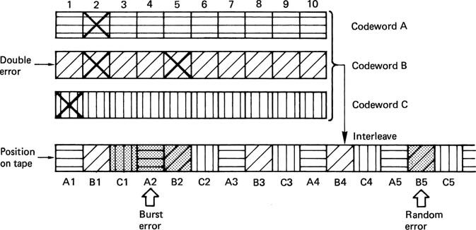
Figure 6.57 shows that in a product code the redundancy calculated first and checked last is called the outer code, and the redundancy calculated second and checked first is called the inner code. The inner code is formed along tracks on the medium. Random errors due to noise are corrected by the inner code and do not impair the burst-correcting power of the outer code. Burst errors are declared uncorrectable by the inner code which flags the bad samples on the way into the de-interleave memory. The outer code reads the error flags in order to correct the flagged symbols by erasure. The error flags are also known as erasure flags. As it does not have to compute the error locations, the outer code needs half as much redundancy for the same correction power. Thus the inner code redundancy does not raise the code overhead. The combination of codewords with interleaving in several dimensions yields an error-protection strategy which is truly synergistic, in that the end result is more powerful than the sum of the parts. Needless to say, the technique is used extensively in modern storage formats.

Figure 6.57 In addition to the redundancy P on rows, inner redundancy Q is also generated on columns. On replay, the Q code checker will pass on flags F if it finds an error too large to handle itself. The flags pass through the de-interleave process and are used by the outer error correction to identify which symbol in the row needs correcting with P redundancy. The concept of crossing two codes in this way is called a product code.

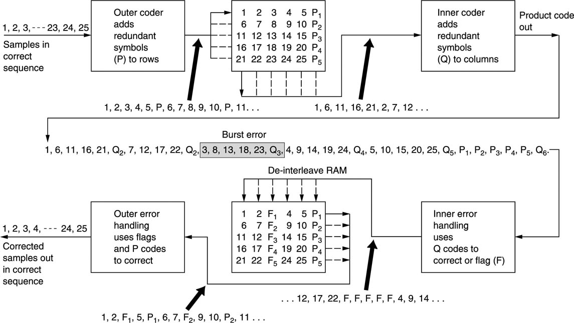
Appendix 6.1 Calculation of Reed–Solomon generator polynomials

For a Reed–Solomon codeword over GF(2³), there will be seven three-bit symbols. For location and correction of one symbol, there must be two redundant symbols P and Q, leaving A–E for data.

The following expressions must be true, where a is the primitive element of x³ ⊕ x ⊕ 1 and ⊕ is XOR throughout:

Dividing equation (2) by a:

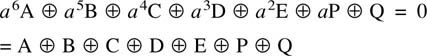
Cancelling Q, and collecting terms:

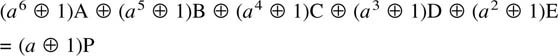
Using section 2.26 to calculate (aⁿ + 1), e.g. a⁶ + 1 = 101 + 001 = 100 = a²;

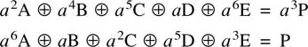
Multiplying equation (1) by a² and equating to equation (2):

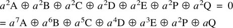
Cancelling terms a²P and collecting terms (remember a² ⊕ a² — 0):

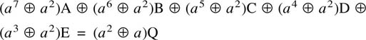
Adding powers according to section 2.26, e.g.

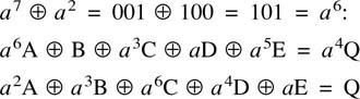
References

1. Deeley, E.M., Integrating and differentiating channels in digital tape recording. Radio Electron. Eng., 56, 169–173 (1986)

2. Mee, C.D., The Physics of Magnetic Recording, Amsterdam and New York: Elsevier–North-Holland Publishing (1978)

3. Jacoby, G.V., Signal equalization in digital magnetic recording. IEEE Trans. Magn., MAG-11, 302–305 (1975)

4. Schneider, R.C., An improved pulse-slimming method for magnetic recording. IEEE Trans. Magn., MAG-11, 1240–1241 (1975)

5. Miller, A., US Patent. No.3 108 261

6. Mallinson, J.C. and Miller, J.W., Optimum codes for digital magnetic recording. Radio and Electron. Eng., 47, 172–176 (1977)

7. Miller, J.W., DC-free encoding for data transmission system. US Patent 4 027 335 (1977)

8. Tang, D.T., Run-length-limited codes. IEEE International Symposium on Information Theory (1969)

9. Yokoyama, K., Digital video tape recorder. NHK Technical Monograph, No.31 (March 1982)

10. Coleman, C.H. et al., High data rate magnetic recording in a single channel. J. IERE, 55, 229–236 (1985)

11. Kobayashi, H., Application of partial response channel coding to magnetic recording systems. IBM J. Res. Dev., 14, 368–375 (1970)

12. Forney, G.D., JR, The Viterbi algorithm, Proc. IEEE, 61, 268–278 (1973)

13. Wood, R.W. and Petersen, D.A., Viterbi detection of Class IV partial response on a magnetic recording channel. IEEE Trans. Commun., 34, 454–461 (1968)

14. Shannon, C.E., A mathematical theory of communication. Bell System Tech. J., 27, 379 (1948)

15. Reed, I.S. and Solomon, G., Polynomial codes over certain finite fields. J. Soc. Indust. Appl. Math., 8, 300–304 (1960)

16. Berlekamp, E.R., Algebraic Coding Theory. New York: McGraw-Hill (1967). Reprint edition: Laguna Hills, CA: Aegean Park Press (1983)

17. Sugiyama, Y. et al., An erasures and errors decoding algorithm for Goppa codes. IEEE Trans. Inf. Theory, IT-22 (1976)

18. Peterson, W.W. and Weldon, E.J., Error Correcting Codes, 2nd edn, Cambridge MA: MIT Press (1972)