
Chapter 4
Digital video processing
The conversion process expresses the analog input as a numerical code. Within the digital domain, all signal processing must be performed by arithmetic manipulation of the code values. Whilst this was at one time done in dedicated logic circuits, the advancing speed of computers means that increasingly the processes explained here will be performed under software control. However, the principles remain the same.
4.1 A simple digital vision mixer
During production, the samples or pixels representing video images need to be mixed with others. Effects such as dissolves and soft-edged wipes can only be achieved if the level of each input signal can be controlled independently. Level is controlled in the digital domain by multiplying every pixel value by a coefficient. If that coefficient is less than one, attenuation will result; if it is greater than one, amplification can be obtained.
Multiplication in binary circuits is difficult. It can be performed by repeated adding, but this is slow. In fast multiplication, one of the inputs will be simultaneously multiplied by one, two, four, etc., by hard-wired bit shifting. Figure 4.1 shows that the other input bits will determine which of these powers will be added to produce the final sum, and which will be neglected. If multiplying by five, the process is the same as multiplying by four, multiplying by one, and adding the two products. This is achieved by adding the input to itself shifted two places. As the wordlength of such a device increases, the complexity increases exponentially, so this is a natural application for an integrated circuit. It is probably true that digital video would not have been viable without such chips.
Figure 4.1 Structure of fast multiplier: the input A is multiplied by 1, 2, 4, 8, etc., by bit shifting. The digits of the B input then determine which multiples of A should be added together by enabling AND gates between the shifters and the adder. For long wordlengths, the number of gates required becomes enormous, and the device is best implemented in a chip.

In a digital mixer, the gain coefficients may originate in hand-operated faders, just as in analog. Analog faders may be retained and used to produce a varying voltage which is converted to a digital code or gain coefficient in an ADC, but it is also possible to obtain coefficients directly in digital faders. Digital faders are a form of displacement transducer known as an encoder in which the mechanical position of the control is converted directly to a digital code. The position of other controls, such as jog wheels on VTRs or editors, will also need to be digitized. Encoders can be linear or rotary, and absolute or relative. In an absolute encoder, the position of the knob determines the output directly. In a relative control, the knob can be moved to increase or decrease the output, but its absolute position is meaningless.
Figure 4.2 shows an absolute linear encoder. A grating is moved with respect to several light beams, one for each bit of the coefficient required. The interruption of the beams by the grating determines which photocells are illuminated. It is not possible to use a pure binary pattern on the grating because this results in transient false codes due to mechanical tolerances. Figure 4.3 shows some examples of these false codes. For example, on moving the fader from 3 to 4, the MSB goes true slightly before the middle bit goes false. This results in a momentary value of 4 + 2 = 6 between 3 and 4. The solution is to use a code in which only one bit ever changes in going from one value to the next. One such code is the Gray code, which was devised to overcome timing hazards in relay logic but is now used extensively in encoders. Gray code can be converted to binary in a suitable PROM or gate array or in software.
Figure 4.2 An absolute linear fader uses a number of light beams which are interrupted in various combinations according to the position of a grating. A Gray code shown in Figure 4.3 must be used to prevent false codes.

Figure 4.3 (a) Binary cannot be used for position encoders because mechanical tolerances cause false codes to be produced. (b) In Gray code, only one bit (arrowed) changes in between positions, so no false codes can be generated.
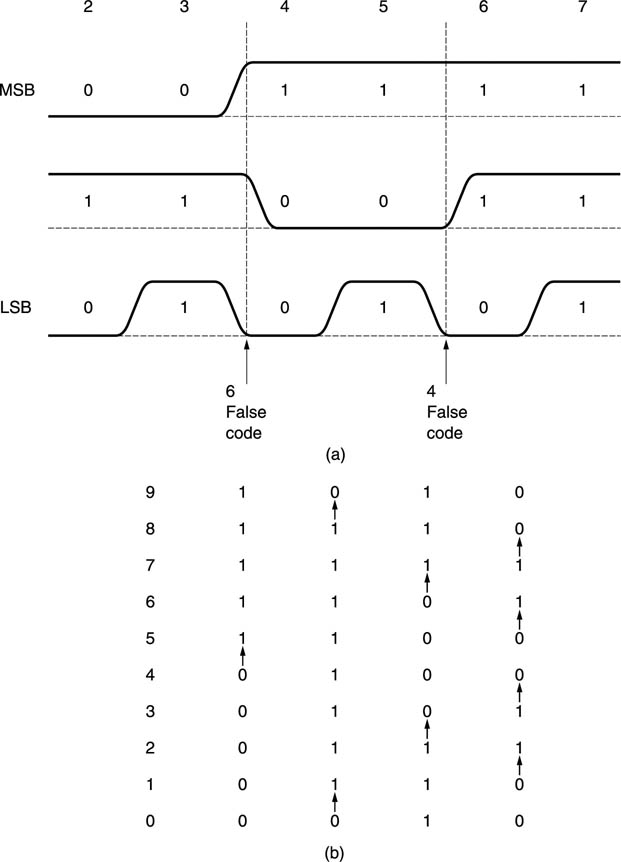
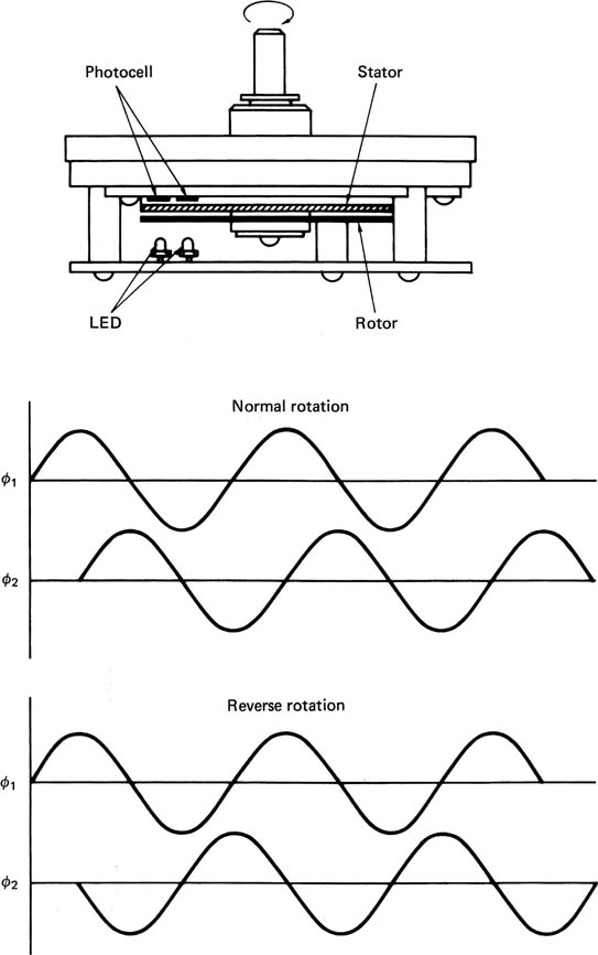
Figure 4.4 shows a rotary incremental encoder. This produces a sequence of pulses whose number is proportional to the angle through which it has been turned. The rotor carries a radial grating over its entire perimeter. This turns over a second fixed radial grating whose bars are not parallel to those of the first grating. The resultant moire fringes travel inward or outward depending on the direction of rotation. Two suitably positioned light beams falling on photocells will produce outputs in quadrature. The relative phase determines the direction and the frequency is proportional to speed. The encoder outputs can be connected to a counter whose contents will increase or decrease according to the direction the rotor is turned. The counter provides the coefficient output.
Figure 4.4 The fixed and rotating gratings produce moiré fringes which are detected by two light paths as quadrature sinusoids. The relative phase determines the direction, and the frequency is proportional to speed of rotation.
The wordlength of the gain coefficients requires some thought as they determine the number of discrete gains available. If the coefficient wordlength is inadequate, the steps in the gain control become obvious particularly towards the end of a fadeout. A compromise between performance and the expense of high-resolution faders is to insert a digital interpolator having a low-pass characteristic between the fader and the gain control stage. This will compute intermediate gains to higher resolution than the coarse fader scale so that the steps cannot be discerned.
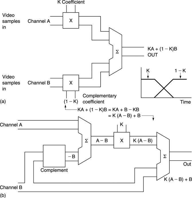
The luminance path of a simple component digital mixer is shown in Figure 4.5. The ITU-601 digital input uses offset binary in that it has a nominal black level of 1610 in an eight-bit pixel, and a subtraction has to be made in order that fading will take place with respect to black. On a perfectly converted signal, subtracting 16 would achieve this, but on a signal subject to a DC offset it would not. Since the digital active line is slightly longer than the analog active line, the first sample should be blanking level, and this will be the value to subtract to obtain pure binary luminance with respect to black. This is the digital equivalent of black level clamping. The two inputs are then multiplied by their respective coefficients, and added together to achieve the mix. Peak limiting will be required as in section 2.13, and then, if the output is to be to ITU-601, 1610 must be added to each sample value to establish the correct offset. In some video applications, a crossfade will be needed, and a rearrangement of the crossfading equation allows one multiplier to be used instead of two, as shown in Figure 4.6.
Figure 4.5 A simple digital mixer. Offset binary inputs must have the offset removed. A digital integrator will produce a counter-offset which is subtracted from every input sample. This will increase or reduce until the output of the subtractor is zero during blanking. The offset must be added back after processing if an ITU-601 output is required.

Figure 4.6 Crossfade at (a) requires two multipliers. Reconfiguration at (b) requires only one multiplier.
The colour difference signals are offset binary with an offset of 12810, and again it is necessary to normalize these with respect to blanking level so that proper fading can be carried out. Since colour difference signals can be positive or negative, this process results in two’s complement samples. Figure 4.7 shows some examples.
Figure 4.7 Offset binary colour difference values are converted to two’s complement by reversing the state of the first bit. Two’s complement values A and B will then add around blanking level.

In this form, the samples can be added with respect to blanking level. Following addition, a limiting stage is used as before, and then, if it is desired to return to ITU-601 standard, the MSB must be inverted once more in order to convert from two’s complement to offset binary.
In practice the same multiplier can be used to process luminance and colour difference signals. Since these will be arriving time multiplexed at 27 MHz, it is only necessary to ensure that the correct coefficients are provided at the right time. Figure 4.8 shows an example of part of a slow fade. As the co-sited samples CB, Y and CR enter, all are multiplied by the same coefficient Kn, but the next sample will be luminance only, so this will be multiplied by Kn+1. The next set of co-sited samples will be multiplied by Kn+2 and so on. Clearly, coefficients must be provided which change at 13.5 MHz. The sampling rate of the two inputs must be exactly the same, and in the same phase, or the circuit will not be able to add on a sample-by-sample basis. If the two inputs have come from different sources, they must be synchronized by the same master clock, and/or timebase correction must be provided on the inputs.
Figure 4.8 When using one multiplier to fade both luminance and colour difference in a 27 MHz multiplex 4:2:2 system, one coefficient will be used three times on the co-sited samples, whereas the next coefficient will only be used for a single luminance sample.

Some thought must be given to the wordlength of the system. If a sample is attenuated, it will develop bits which are below the radix point. For example, if an eight-bit sample is attenuated by 24 dB, the sample value will be shifted four places down. Extra bits must be available within the mixer to accommodate this shift. Digital vision mixers may have an internal wordlength of sixteen bits or more. When several attenuated sources are added together to produce the final mix, the result will be a sixteen-bit sample stream. As the output will generally need to be of the same format as the input, the wordlength must be shortened.
Shortening the wordlength of samples effectively makes the quantizing intervals larger and Chapter 3 showed that this can be called requantizing. This must be done using digital dithering to avoid artifacts.
4.2 Keying
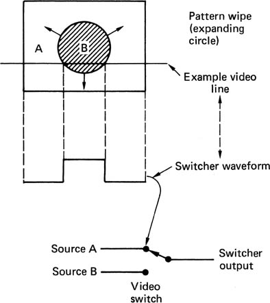
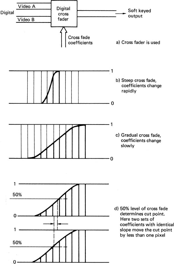
Keying is the process where one video signal can be cut into another to replace part of the picture with a different image. One application of keying is where a switcher can wipe from one input to another using one of a variety of different patterns. Figure 4.9 shows that an analog switcher performs such an effect by generating a binary switching waveform in a pattern generator. Video switching between inputs actually takes place during the active line. In most analog switchers, the switching waveform is digitally generated, then fed to a D-A convertor, whereas in a digital switcher, the pattern generator outputs become the coefficients supplied to the crossfader, which is sometimes referred to as a cutter. The switching edge must be positioned to an accuracy of a few nanoseconds, much less than the spacing of the pixels, otherwise slow wipes will not appear to move smoothly, and diagonal wipes will have stepped edges, a phenomenon known as ratcheting.
Figure 4.9 In a video switcher a pattern generator produces a switching waveform which changes from line to line and from frame to frame to allow moving pattern wipes between sources.
Positioning the switch point to sub-pixel accuracy is not particularly difficult, as Figure 4.10 shows. A suitable series of coefficients can position the effective crossover point anywhere. The finite slope of the coefficients results in a brief crossfade from one video signal to the other. This soft-keying gives a much more realistic effect than binary switchers, which often give a ‘cut out with scissors’ appearance. In some machines the slope of the crossfade can be adjusted to achieve the desired degree of softness.
Figure 4.10 Soft keying.
Another application of keying is to derive the switching signal by processing video from a camera in some way. By analysing colour difference signals, it is possible to determine where in a picture a particular colour occurs. When a key signal is generated in this way, the process is known as chroma keying, which is the electronic equivalent of matting in film.
In a 4:2:2 component system, It will be necessary to provide coefficients to the luminance crossfader at 13.5 MHz. Chroma samples only occur at half this frequency, so it is necessary to provide a chroma interpolator to artificially raise the chroma sampling rate. For chroma keying a simple linear interpolator is perfectly adequate.
As with analog switchers, chroma keying is also possible with composite digital inputs, but decoding must take place before it is possible to obtain the key signals. The video signals which are being keyed will, however, remain in the composite digital format.
In switcher/keyers, it is necessary to obtain a switching signal which ramps between two states from an input signal which can be any allowable video waveform. Manual controls are provided so that the operator can set thresholds and gains to obtain the desired effect. In the analog domain, these controls distort the transfer function of a video amplifier so that it is no longer linear. A digital keyer will perform the same functions using logic circuits.
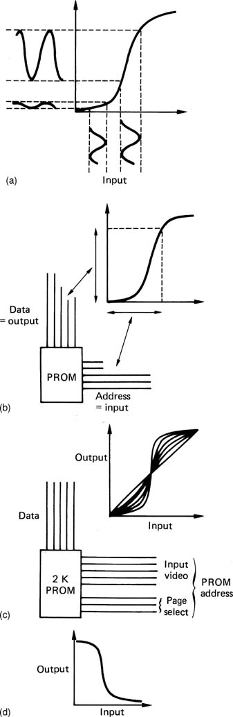
Figure 4.11(a) shows the effect of a non-linear transfer function is to switch when the input signal passes through a particular level. The transfer function is implemented in a memory in digital systems. The incoming video sample value acts as the memory address, so that the selected memory location is proportional to the video level. At each memory location, the appropriate output level code is stored. If, for example, each memory location stored its own address, the output would equal the input, and the device would be transparent. In practice, switching is obtained by distorting the transfer function to obtain more gain in one particular range of input levels at the expense of less gain at other input levels. With the transfer function shown in Figure 4.11(b), an input level change from a to b causes a smaller output change, whereas the same level change between c and d causes a considerable output change.
Figure 4.11 (a) A non-linear transfer function can be used to produce a keying signal. (b) The non-linear transfer function emphasizes contrast in part of the range but reduces it at other parts. (c) If a RAM is used as a flexible transfer function, it will be necessary to provide multiplexers so that the RAM can be preset with the desired values from the control system.

If the memory is RAM, different transfer functions can be loaded in by the control system, and this requires multiplexers in both data and address lines as shown in Figure 4.11(c). In practice such a RAM will be installed in Y, Cr and Cb channels, and the results will be combined to obtain the final switching coefficients.
4.3 Digital video effects
If a RAM of the type shown in Figure 4.11 is inserted in a digital luminance path, the result will be solarizing, which is a form of contrast enhancement. Figure 4.12 shows that a family of transfer functions can be implemented which control the degree of contrast enhancement. When the transfer function becomes so distorted that the slope reverses, the result is luminance reversal, where black and white are effectively interchanged. Solarizing can also be implemented in colour difference channels to obtain chroma solarizing. In effects machines, the degree of solarizing may need to change smoothly so that the effect can be gradually introduced. In this case the various transfer functions will be kept in different pages of a PROM, so that the degree of solarization can be selected immediately by changing the page address of the PROM. One page will have a straight transfer function, so the effect can be turned off by selecting that page.
Figure 4.12 Solarization. (a) The non-linear transfer function emphasizes contrast in part of the range but reduces it at other parts. (b) The desired transfer function is implemented in a PROM. Each input sample value is used as the address to select a corresponding output value stored in the PROM. (c) A family of transfer functions can be accommodated in a larger PROM. Page select affects the high-order address bits. (d) Transfer function for luminance reversal.
In the digital domain it is easy to introduce various forms of quantizing distortion to obtain special effects. Figure 4.13 shows that eight-bit luminance allows 256 different brightnesses, which to the naked eye appears to be a continuous range. If some of the low-order bits of the samples are disabled, then a smaller number of brightness values describes the range from black to white. For example, if six bits are disabled, only two bits remain, and so only four possible brightness levels can be output. This gives an effect known as contouring since the visual effect somewhat resembles a relief map.
When the same process is performed with colour difference signals, the result is to limit the number of possible colours in the picture, which gives an effect known as posterizing, since the picture appears to have been coloured by paint from pots. Solarizing, contouring and posterizing cannot be performed in the composite digital domain, owing to the presence of the subcarrier in the sample values.
Figure 4.13 (a) In contouring, the least significant bits of the luminance samples are discarded, which reduces the number of possible output levels. (b) At left, the eight-bit colour difference signals allow 216 different colours. At right, eliminating all but two bits of each colour difference signals allows only 24 different colours.

Figure 4.14 shows a latch in the luminance data which is being clocked at the sampling rate. It is transparent to the signal, but if the clock to the latch is divided down by some factor n, the result will be that the same sample value will be held on the output for n clock periods, giving the video waveform a staircase characteristic. This is the horizontal component of the effect known as mosaicing. The vertical component is obtained by feeding the output of the latch into a line memory, which stores one horizontally mosaiced line and then repeats that line m times. As n and m can be independently controlled, the mosaic tiles can be made to be of any size, and rectangular or square at will. Clearly, the mosaic circuitry must be implemented simultaneously in luminance and colour difference signal paths. It is not possible to perform mosaicing on a composite digital signal, since it will destroy the subcarrier. It is common to provide a bypass route which allows mosaiced and unmosaiced video to be simultaneously available. Dynamic switching between the two sources controlled by a separate key signal then allows mosaicing to be restricted to certain parts of the picture.
Figure 4.14 (a) Simplified diagram of mosaicing system. At the left-hand side, horizontal mosaicing is done by intercepting sample clocks. On one line in m, the horizontally mosaiced line becomes the output, and is simultaneously written into a one-line memory. On the remaining (m-1) lines the memory is read to produce several identical successive lines to give the vertical dimensions of the tile. (b) In mosaicing, input samples are neglected, and the output is held constant by failing to clock a latch in the data stream for several sample periods. Heavy vertical lines here correspond to the clock signal occurring. Heavy horizontal line is resultant waveform.

The above simple effects did not change the shape or size of the picture, whereas the following class of manipulations will. Effects machines which manipulate video pictures are close relatives of the machines that produce computer-generated images.
The principle of all video manipulators is the same as the technique used by cartographers for centuries. Cartographers are faced with a continual problem in that the earth is round, and paper is flat. In order to produce flat maps, it is necessary to project the features of the round original onto a flat surface. Figure 4.15 shows an example of this. There are a number of different ways of projecting maps, and all of them must by definition produce distortion. The effect of this distortion is that distances measured near the extremities of the map appear further than they actually are. Another effect is that great circle routes (the shortest or longest path between two places on a planet) appear curved on a projected map. The type of projection used is usually printed somewhere on the map, a very common system being that due to Mercator. Clearly, the process of mapping involves some three-dimensional geometry in order to simulate the paths of light rays from the map so that they appear to have come from the curved surface. Video effects machines work in exactly the same way.
Figure 4.15 Map projection is a close relative of video effects units which manipulate the shape of pictures.

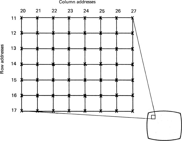
The distortion of maps means that things are not where they seem. In timesharing computers, every user appears to have his or her own identical address space in which the program resides, despite the fact that many different programs are simultaneously in the memory. In order to resolve this contradiction, memory management units are constructed which add a constant value to the address which the user thinks he has (the virtual address) in order to produce the physical address. As long as the unit gives each user a different constant, they can all program in the same virtual address space without one corrupting another’s programs. Because the program is no longer where it seems to be, the term of ‘mapping’ was introduced. The address space of a computer is one-dimensional, but a video frame expressed as rows and columns of pixels can be considered to have a two-dimensional address as in Figure 4.16. Video manipulators work by mapping the pixel addresses in two dimensions.
Figure 4.16 The entire TV picture can be broken down into uniquely addressable pixels.
All manipulators must begin with an array of pixels, in which the columns must be vertical. This can only be easily obtained if the sampling rate of the incoming video is a multiple of line rate, as is done in ITU-601. Composite video cannot be used directly, because the phase of the subcarrier would become meaningless after manipulation. If a composite video input is used, it must be decoded to baseband luminance and colour difference, so that in actuality there are three superimposed arrays of samples to be processed, one luminance, and two colour difference. Most production DVEs use ITU-601 sampling, so digital signals conforming to this standard could be used directly, from, for example, a DVTR or a hard-disk recorder.
DVEs work best with progressively scanned material and the use of interlace causes some additional problems. A DVE designed to work with interlaced inputs must de-interlace first so that all the vertical resolution information is available in every image to be mapped. The most accurate de-interlacing requires motion compensation which is considered in section 4.7.
The additional cost and complexity of de-interlacing is substantial, but this is essential for post-production work, where the utmost quality is demanded. Where low cost is the priority, a field-based DVE system may be acceptable.
The effect of de-interlacing is to produce an array of pixels which are the input data for the processor. In 13.5 MHz systems, the array will be about 720 pixels across and 600 down for 50 Hz systems, 500 down for 60 Hz systems. Most machines are set to strip out VITC or teletext data from the input, so that pixels representing genuine picture appear surrounded by blanking level.
Every pixel in the frame array has an address. The address is two-dimensional, because in order to uniquely specify one pixel, the column address and the row address must be supplied. It is possible to transform a picture by simultaneously addressing in rows and columns, but this is complicated, and very difficult to do in real time. It was discovered some time ago in connection with computer graphics that the two-dimensional problem can be converted with care into two one-dimensional problems.1 Essentially if a horizontal transform affecting whole rows of pixels independently of other rows is performed on the array, followed by or preceded by a vertical transform which affects entire columns independently of other columns, the effect will be the same as if a two-dimensional transform had been performed. This is the principle of separability. From an academic standpoint, it does not matter which transform is performed first. In a world which is wedded to the horizontally scanned television set, there are practical matters to consider. In order to convert a horizontal raster input into a vertical column format, a memory is needed where the input signal is written in rows, but the output is read as columns of pixels.
The process of writing rows and reading columns in a memory is called transposition. Clearly, two stages of transposition are necessary to return to a horizontal raster output, as shown in Figure 4.17. The vertical transform must take place between the two transposes, but the horizontal transform could take place before the first transpose or after the second one. In practice, the horizontal transform cannot be placed before the first transpose, because it would interfere with the de-interlace and motion-sensing process. The horizontal transform is placed after the second transpose, and reads rows from the second transpose memory. As the output of the machine must be a horizontal raster, the horizontal transform can be made to work in synchronism with reference H-sync so that the digital output samples from the H-transform can be taken direct to a DAC to become analog video with a standard structure again. A further advantage is that the real-time horizontal output is one field at a time. The preceding vertical transform need only compute array values which lie in the next field to be needed at the output.
Figure 4.17 Two transposing memories are necessary, one before and one after the vertical transform.

It is not possible to take a complete column from a memory until all the rows have entered. The presence of the two transposes in a DVE results in an unavoidable delay of one frame in the output image. Some DVEs can manage greater delay. The effect on lip-sync may have to be considered. It is not advisable to cut from the input of a DVE to the output, since a frame will be lost, and on cutting back a frame will be repeated.
Address mapping is used to perform transforms. Now that rows and columns are processed individually, the mapping process becomes much easier to understand. Figure 4.18 shows a single row of pixels which are held in a buffer where each can be addressed individually and transferred to another. If a constant is added to the read address, the selected pixel will be to the right of the place where it will be put. This has the effect of moving the picture to the left. If the buffer represented a column of pixels, the picture would be moved vertically. As these two transforms can be controlled independently, the picture could be moved diagonally.
If the read address is multiplied by a constant, say 2, the effect is to bring samples from the input closer together on the output, so that the picture size is reduced. Again independent control of the horizontal and vertical transforms is possible, so that the aspect ratio of the picture can be modified. This is very useful for telecine work when CinemaScope films are to be broadcast. Clearly the secret of these manipulations is in the constants fed to the address generators. The added constant represents displacement, and the multiplied constant represents magnification. A multiplier constant of less than one will result in the picture getting larger. Figure 4.18 also shows, however, that there is a problem. If a constant of 0.5 is used, to make the picture twice as big, half of the addresses generated are not integers. A memory does not understand an address of two and a half!)
Figure 4.18 Address generation is the fundamental process behind transforms.

If an arbitrary magnification is used, nearly all the addresses generated are non-integer. A similar problem crops up if a constant of less than one is added to the address in an attempt to move the picture less than the pixel spacing. The solution to the problem is interpolation. Because the input image is spatially sampled, those samples contain enough information to represent the brightness and colour all over the screen. When the address generator comes up with an address of 2.5, it actually means that what is wanted is the value of the signal interpolated half-way between pixel two and pixel three. The output of the address generator will thus be split into two parts. The integer part will become the memory address, and the fractional part is the phase of the necessary interpolation. In order to interpolate pixel values a digital filter is necessary.
Figure 4.19 shows that the input and output of an effects machine must be at standard sampling rates to allow digital interchange with other equipment. When the size of a picture is changed, this causes the pixels in the picture to fail to register with output pixel spacing. The problem is exactly the same as sampling rate conversion, which produces a differently spaced set of samples that still represent the original waveform. One pixel value actually represents the peak brightness of a two-dimensional intensity function, which is the effect of the modulation transfer function of the system on an infinitely small point. As each dimension can be treated separately, the equivalent in one axis is that the pixel value represents the peak value of an infinitely short impulse which has been low-pass filtered to the system bandwidth and windowed.
Figure 4.19 It is easy, almost trivial, to reduce the size of a picture by pushing the samples closer together, but this is not often of use, because it changes the sampling rate in proportion to the compression. Where a standard sampling-rate output is needed, interpolation must be used.

In order to compute an interpolated value, it is necessary to add together the contribution from all relevant samples, at the point of interest. Each contribution can be obtained by looking up the value of the impulse response at the distance from the input pixel to the output pixel to obtain a coefficient, and multiplying the input pixel value by that coefficient. The process of taking several pixel values, multiplying each by a different coefficient and summing the products can be performed by the FIR (finite impulse response) configuration described in Chapter 2. The impulse response of the filter necessary depends on the magnification. Where the picture is being enlarged, the impulse response can be the same as at normal size, but as the size is reduced, the impulse response has to become broader (corresponding to a reduced spatial frequency response) so that more input samples are averaged together to prevent aliasing. The coefficient store will need a two-dimensional structure, such that the magnification and the interpolation phase must both be supplied to obtain a set of coefficients. The magnification can easily be obtained by comparing successive outputs from the address generator.
The number of points in the filter is a compromise between cost and performance, eight being a typical number for high quality. As there are two transform processes in series, every output pixel will be the result of sixteen multiplications, so there will be 216 million multiplications per second taking place in the luminance channel alone for a 13.5 MHz sampling rate unit. The quality of the output video also depends on the number of different interpolation phases available between pixels. The address generator may compute fractional addresses to any accuracy, but these will be rounded off to the nearest available phase in the digital filter. The effect is that the output pixel value provided is actually the value a tiny distance away, and has the same result as sampling clock jitter, which is to produce program-modulated noise. The greater the number of phases provided, the larger will be the size of the coefficient store needed. As the coefficient store is two-dimensional, an increase in the number of filter points and phases causes an exponential growth in size and cost.
In order to follow the operation of a true perspective machine, some knowledge of perspective is necessary. Stated briefly, the phenomenon of perspective is due to the angle subtended to the eye by objects being a function not only of their size but also of their distance. Figure 4.20 shows that the size of an image on the rear wall of a pinhole camera can be increased either by making the object larger or bringing it closer. In the absence of stereoscopic vision, it is not possible to tell which has happened. The pinhole camera is very useful for study of perspective, and has indeed been used by artists for that purpose. The clinically precise perspective of Canaletto paintings was achieved through the use of the camera obscura (Latin: darkened room).2
Figure 4.20 The image on the rear of the pinhole camera is identical for the two solid objects shown because the size of the object is proportional to distance, and the subtended angle remains the same. The image can be made larger (dotted) by making the object larger or moving it closer.

It is sometimes claimed that the focal length of the lens used on a camera changes the perspective of a picture. This is not true, perspective is only a function of the relative positions of the camera and the subject. Fitting a wide-angle lens simply allows the camera to come near enough to keep dramatic perspective within the frame, whereas fitting a long-focus lens allows the camera to be far enough away to display a reasonably sized image with flat perspective.3
Since a single eye cannot tell distance unaided, all current effects machines work by simply producing the correct subtended angles which the brain perceives as a three-dimensional effect. Figure 4.21 shows that to a single eye, there is no difference between a three-dimensional scene and a two-dimensional image formed where rays traced from features to the eye intersect an imaginary plane. This is exactly the reverse of the map projection shown in Figure 4.15, and is the principle of all perspective manipulators.
Figure 4.21 In a planar rotation effect the source plane ABCD is the rectangular input picture. If it is rotated through the angle Θ, ray tracing to a single eye at left will produce a trapezoidal image A’B’C’D’ on the target. Magnification will now vary with position on the picture.
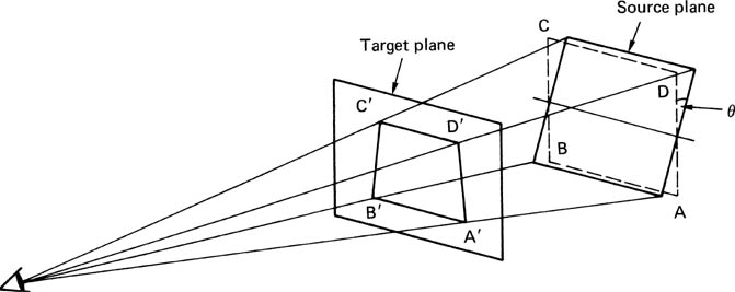
The case of perspective rotation of a plane source will be discussed first. Figure 4.21 shows that when a plane input frame is rotated about a horizontal axis, the distance from the top of the picture to the eye is no longer the same as the distance from the bottom of the picture to the eye. The result is that the top and bottom edges of the picture subtend different angles to the eye, and where the rays cross the target plane, the image has become trapezoidal. There is now no such thing as the magnification of the picture. The magnification changes continuously from top to bottom of the picture, and if a uniform grid is input, after a perspective rotation it will appear non-linear, as the diagram shows.
The basic mechanism of the transform process has been described, but this is only half of the story, because these transforms have to be controlled. There is a lot of complex geometrical calculation necessary to perform even the simplest effect, and the operator cannot be expected to calculate directly the parameters required for the transforms. All effects machines require a computer of some kind, with which the operator communicates using keyboard entry or joystick/trackball movements at high level. These high-level commands will specify such things as the position of the axis of rotation of the picture relative to the viewer, the position of the axis of rotation relative to the source picture, and the angle of rotation in the three axes.
An essential feature of this kind of effects machines is fluid movement of the source picture as the effect proceeds. If the source picture is to be made to move smoothly, then clearly the transform parameters will be different in each field. The operator cannot be expected to input the source position for every field, because this would be an enormous task. Additionally, storing the effect would require a lot of space. The solution is for the operator to specify the picture position at strategic points during the effect, and then digital filters are used to compute the intermediate positions so that every field will have different parameters.
The specified positions are referred to as knots, nodes or keyframes, the first being the computer graphics term. The operator is free to enter knots anywhere in the effect, and so they will not necessarily be evenly spaced in time, i.e. there may well be different numbers of fields between each knot. In this environment it is not possible to use conventional FIR-type digital filtering, because a fixed impulse response is inappropriate for irregularly spaced samples.
Interpolation of various orders is used ranging from zero-order hold for special jerky effects through linear interpolation to cubic interpolation for very smooth motion. The algorithms used to perform the interpolation are known as splines, a term which has come down from shipbuilding via computer graphics.4 When a ship is designed, the draughtsman produces hull cross-sections at intervals along the keel, whereas the shipyard needs to re-create a continuous structure. The solution was a lead-filled bar, known as a spline, which could be formed to join up each cross-section in a smooth curve, and then used as a template to form the hull plating.
The filter which does not ring cannot be made, and so the use of spline algorithms for smooth motion sometimes results in unintentional overshoots of the picture position. This can be overcome by modifying the filtering algorithm. Spline algorithms usually look ahead beyond the next knot in order to compute the degree of curvature in the graph of the parameter against time. If a break is put in that parameter at a given knot, the spline algorithm is prevented from looking ahead, and no overshoot will occur. In practice, the effect is created and run without breaks, and then breaks are added later where they are subjectively thought necessary.
It will be seen that there are several levels of control in an effects machine. At the highest level, the operator can create, store and edit knots, and specify the times which elapse between them. The next level is for the knots to be interpolated by spline algorithms to produce parameters for every field in the effect. The field frequency parameters are then used as the inputs to the geometrical computation of transform parameters which the lowest level of the machine will use as microinstructions to act upon the pixel data. Each of these layers will often have a separate processor, not just for speed, but also to allow software to be updated at certain levels without disturbing others.
4.4 Graphics
Although there is no easy definition of a video graphics system which distinguishes it from a graphic art system, for the purposes of discussion it can be said that graphics consists of generating alphanumerics on the screen, whereas graphic art is concerned with generating more general images. The simplest form of screen presentation of alphanumerics is the ubiquitous visual display unit (VDU) which is frequently necessary to control computer-based systems. The mechanism used for character generation in such devices is very simple, and thus makes a good introduction to the subject.
In VDUs, there is no grey scale, and the characters are formed by changing the video signal between two levels at the appropriate place in the line. Figure 4.22 shows how a character is built up in this way, and also illustrates how easy it is to obtain the reversed video used in some word processor displays to simulate dark characters on white paper. Also shown is the method of highlighting single characters or words by using localized reverse video.
Figure 4.22 Elementary character generation. At (a), white on black waveform for two raster lines passing through letter A. At (b), black on white is simple inversion. At (c), reverse video highlight waveforms.
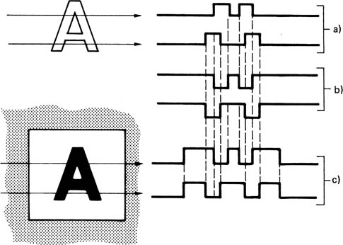
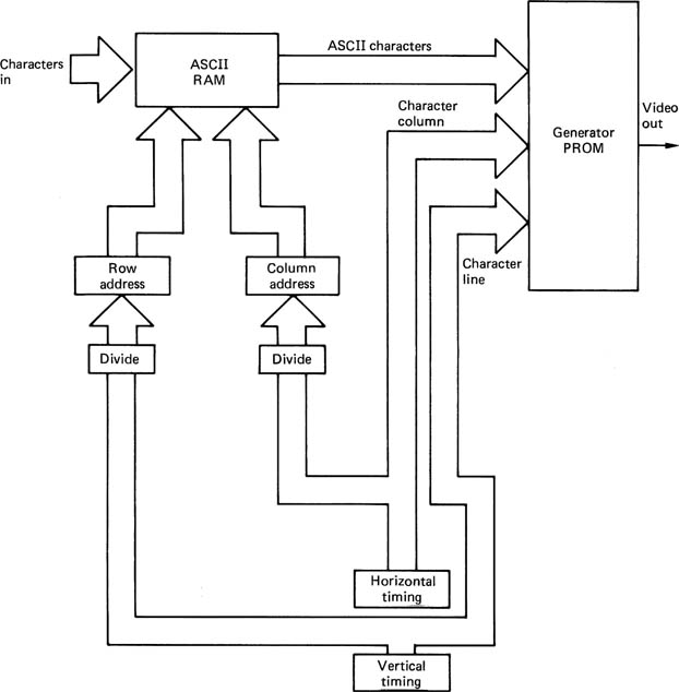
Figure 4.23 is a representative character generator, as might be used in a VDU. The characters to be displayed are stored as ASCII symbols in a RAM, which has one location for each character position on each available text line on the screen. Each character must be used to generate a series of dots on the screen which will extend over several lines. Typically the characters are formed by an array five dots by nine. In order to convert from the ASCII code to a dot pattern, a ROM is programmed with a conversion. This will be addressed by the ASCII character, and the column and row addresses in the character array, and will output a high or low (bright or dark) output.
As the VDU screen is a raster-scanned device, the display scan will begin at the left-hand end of the top line. The first character in the ASCII RAM will be selected, and this and the first row and column addresses will be sent to the character generator, which ouputs the video level for the first pixel. The next column address will then be selected, and the next pixel will be output. As the scan proceeds, it will pass from the top line of the first character to the top line of the second character, so that the ASCII RAM address will need to be incremented. This process continues until the whole video line is completed. The next line on the screen is generated by repeating the selection of characters from the ASCII RAM, but using the second array line as the address to the character generator. This process will repeat until all the video lines needed to form one row of characters are complete. The next row of characters in the ASCII RAM can then be accessed to create the next line of text on the screen and so on.
Figure 4.23 Simple character generator produces characters as rows and columns of pixels. See text for details.
The character quality of VDUs is adequate for the application, but is not satisfactory for high-quality broadcast graphics. The characters are monochrome, have a fixed, simple font, fixed size, no grey scale, and the sloping edges of the characters have the usual stepped edges due to the lack of grey scale. This stepping of diagonal edges is sometimes erroneously called aliasing. Since it is a result not of inadequate sampling rate, but of quantizing distortion, the use of the term is wholly inappropriate.
In a broadcast graphics unit, the characters will be needed in colour, and in varying sizes. Different fonts will be necessary, and additional features such as solid lines around characters and drop shadows are desirable. The complexity and cost of the necessary hardware is much greater than in the previous example.
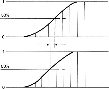
In order to generate a character in a broadcast machine, a font and the character within that font are selected. The characters are actually stored as key signals, because the only difference between one character and another in the same font is the shape. A character is generated by specifying a constant background colour and luminance, and a constant character colour and luminance, and using the key signal to cut a hole in the background and insert the character colour. This is illustrated in Figure 4.24. The problem of stepped diagonal edges is overcome by giving the key signal a grey scale which eliminates the quantizing distortion responsible for the stepped edges. The edge of the character now takes the form of a ramp, which has the desirable characteristic of limiting the bandwidth of the character generator output. Early character generators were notorious for producing out-of-band frequencies which drove equipment further down the line to distraction and in some cases would interfere with the sound channel on being broadcast. Figure 4.25 illustrates how in a system with grey scale and sloped edges, the edge of a character can be positioned to sub-pixel resolution, which completely removes the stepped effect on diagonals.
Figure 4.24 Font characters only store the shape of the character. This can be used to key any coloured character into a background.

Figure 4.25 When a character has a ramped edge, the edge position can be moved in subpixel steps by changing the pixel values in the ramp.
In a powerful system, the number of fonts available will be large, and all the necessary characters will be stored on disk drives. Some systems allow users to enter their own fonts using a rostrum camera. A frame grab is performed, but the system can be told to file the image as a font character key signal rather than as a still frame. This approach allows infinite flexibility if it is desired to work in Kanji or Cyrillic, and allows European graphics to be done with all necessary umlauts, tildes and cedillas.
In order to create a character string on the screen, it is necessary to produce a key signal which has been assembled from all the individual character keys. The keys are usually stored in a large format to give highest quality, and it will be necessary to reduce the size of the characters to fit the available screen area. The size reduction of a key signal in the digital domain is exactly the same as the zoom function of an effects machine, requiring FIR filtering and interpolation, but again, it is not necessary for it to be done in real time, and so less hardware can be used. The key source for the generation of the final video output is a RAM which has one location for every screen pixel. Position of the characters on the screen is controlled by changing the addresses in the key RAM into which the size reduced character keys are written.
The keying system necessary is shown in Figure 4.26. The character colour and the background colour are produced by latches on the control system bus, which output continuous digital parameters. The grey scale key signal obtained by scanning the key memory is used to provide coefficients for the digital crossfader which cuts between background and character colour to assemble the video signal in real time.
Figure 4.26 Simple character generator using keying. See text for details.

If characters with contrasting edges are required, an extra stage of keying can be used. The steps described above take place, but the background colour is replaced by the desired character edge colour. The size of each character key is then increased slightly, and the new key signal is used to cut the characters and a contrasting border into the final background.
Early character generators were based on a frame store which refreshes the dynamic output video. Recent devices abandon the framestore approach in favour of real-time synthesis. The symbols which make up a word can move on and turn with respect to the plane in which they reside as a function of time in any way individually or together. Text can also be mapped onto an arbitrarily shaped line. The angle of the characters can follow a tangent to the line, or can remain at a fixed angle regardless of the line angle.
By controlling the size of planes, characters or words can appear to zoom into view from a distance and recede again. Rotation of the character planes off the plane of the screen allows the perspective effects to be seen. Rotating a plane back about a horizontal axis by 90° will reduce it to an edge-on line, but lowering the plane to the bottom of the screen allows the top surface to be seen, receding into the distance like a road. Characters or text strings can then roll off into the distance, getting smaller as they go. In fact the planes do not rotate, but a perspective transform is performed on them.
Since characters can be moved without restriction, it will be possible to make them overlap. Either one can be declared to be at the front, so that it cuts out the other, but if desired the overlapping area can be made a different colour from either of the characters concerned. If this is done with care, the overlapping colour will give the effect of transparency. In fact colour is attributed to characters flexibly so that a character may change colour with respect to time. If this is combined with a movement, the colour will appear to change with position. The background can also be allocated a colour in this way, or the background can be input video. Instead of filling characters with colour on a video background, the characters, or only certain characters, or only the overlapping areas of characters can be filled with video.
There will be several planes on which characters can move, and these are assigned a priority sequence so that the first one is essentially at the front of the screen and the last one is at the back. Where no character exists, a plane is transparent, and every character on a plane has an eight-bit transparency figure allocated to it. When characters on two different planes are moved until they overlap, the priority system and the transparency parameter decide what will be seen. An opaque front character will obscure any character behind it, whereas using a more transparent parameter will allow a proportion of a character to be seen through one in front of it. Since characters have multi-bit accuracy, all transparency effects are performed without degradation, and character edges always remain smooth, even at overlaps. Clearly, the character planes are not memories or frame stores, because perspective rotation of images held in frame stores in real time in this way would require staggering processing power. Instead, the contents of output fields are computed in real time. Every field is determined individually, so it is scarcely more difficult to animate by making successive fields different.
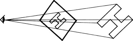
In a computer a symbol or character exists not as an array of pixels, but as an outline, rather as if a thin wire frame had been made to fit the edge of the symbol. The wire frame is described by a set of mathematical expressions. The operator positions the wire frame in space, and turns it to any angle. The computer then calculates what the wire frame will look like from the viewing position. Effectively the shape of the frame is projected onto a surface which will become the TV screen. The principle is shown in Figure 4.27, and will be seen to be another example of mapping. If drop or plane shadows are being used, a further projection takes place which determines how the shadow of the wire frame would fall on a second plane. The only difference here between drop and plane shadows is the angle of the plane the shadow falls on. If it is parallel to the symbol frame, the result is a drop shadow. If it is at right angles, the result is a plane shadow.
Figure 4.27 Perspective effects results from mapping or projecting the character outline on to a plane which represents the screen.
Since the wire frame can be described by a minimum amount of data, the geometrical calculations needed to project onto the screen and shadow planes are quick, and are repeated for every symbol. This process also reveals where overlaps occur within a plane, since the projected frames will cross each other. This computation takes place for all planes. The positions of the symbol edges are then converted to a pixel array in a field-interlaced raster scan. Because the symbols are described by eight-bit pixels, edges can be positioned to sub-pixel accuracy. An example is shown in Figure 4.28. The pixel sequence is now effectively a digital key signal, and the priority and transparency parameters are now used to reduce the amplitude of a given key when it is behind a symbol on a plane of higher priority which has less than 100 per cent transparency.
Figure 4.28 The eight-bit resolution of pixels allows the edge of characters to be placed accurately independent of the sampling points. This offers smooth character edges.

The key signals then pass to a device known as the filler which is a fast digital mixer that has as inputs the colour of each character, and the background, whether colour or video. On a pixel-by-pixel basis, the filler crossfades between different colours as the video line proceeds. The crossfading is controlled by the key signals. The output is three data streams, red, green and blue. The output board takes the data and converts them to the video standard needed, and the result can then be seen.
In graphic art systems, there is a requirement for disk storage of the generated images, and some art machines incorporate a still store unit, whereas others can be connected to a separate one by an interface. Disk-based stores are discussed in Chapter 7. The essence of an art system is that an artist can draw images which become a video signal directly with no intermediate paper and paint. Central to the operation of most art systems is a digitizing tablet, which is a flat surface over which the operator draws a stylus. The tablet can establish the position of the stylus in vertical and horizontal axes. One way in which this can be done is to launch ultrasonic pulses down the tablet, which are detected by a transducer in the stylus. The time taken to receive the pulse is proportional to the distance to the stylus. The coordinates of the stylus are converted to addresses in the frame store which correspond to the same physical position on the screen. In order to make a simple sketch, the operator specifies a background parameter, perhaps white, which would be loaded into every location in the frame store. A different parameter is then written into every location addressed by movement of the stylus, which results in a line drawing on the screen. The art world uses pens and brushes of different shapes and sizes to obtain a variety of effects, one common example being the rectangular pen nib where the width of the resulting line depends on the angle at which the pen is moved. This can be simulated on art systems, because the address derived from the tablet is processed to produce a range of addresses within a certain screen distance of the stylus. If all these locations are updated as the stylus moves, a broad stroke results.
If the address range is larger in the horizontal axis than in the vertical axis, for example, the width of the stroke will be a function of the direction of stylus travel. Some systems have a sprung tip on the stylus which connects to a force transducer, so that the system can measure the pressure the operator uses. By making the address range a function of pressure, broader strokes can be obtained simply by pressing harder. In order to simulate a set of colours available on a palette, the operator can select a mode where small areas of each colour are displayed in boxes on the monitor screen. The desired colour is selected by moving a screen cursor over the box using the tablet. The parameter to be written into selected locations in the frame RAM now reflects the chosen colour. In more advanced systems, simulation of airbrushing is possible. In this technique, the transparency of the stroke is great at the edge, where the background can be seen showing through, but transparency reduces to the centre of the stroke. A readmodify-write process is necessary in the frame memory, where background values are read, mixed with paint values with the appropriate transparency, and written back. The position of the stylus effectively determines the centre of a two-dimensional transparency contour, which is convolved with the memory contents as the stylus moves.
4.5 Applications of motion compensation
Section 2.10 introduced the concept of eye tracking and the optic flow axis. The optic flow axis is the locus of some point on a moving object which will be in a different place in successive pictures. Any device which computes with respect to the optic flow axis is said to be motion compensated. Until recently the amount of computation required in motion compensation was too expensive, but now this is no longer the case the technology has become very important in moving-image portrayal systems.
Figure 4.29(a) shows an example of a moving object which is in a different place in each of three pictures. The optic flow axis is shown. The object is not moving with respect to the optic flow axis and if this axis can be found some very useful results are obtained. The process of finding the optic flow axis is called motion estimation. Motion estimation is literally a process which analyses successive pictures and determines how objects move from one to the next. It is an important enabling technology because of the way it parallels the action of the human eye.
Figure 4.29(b) shows that if the object does not change its appearance as it moves, it can be portrayed in two of the pictures by using data from one picture only, simply by shifting part of the picture to a new location. This can be done using vectors as shown. Instead of transmitting a lot of pixel data, a few vectors are sent instead. This is the basis of motion-compensated compression which is used extensively in MPEG, as will be seen in Chapter 5.
Figure 4.29 Motion compensation is an important technology. (a) The optic flow axis is found for a moving object. (b) The object in picture (n + 1) and (n + 2) can be re-created by shifting the object of picture n using motion vectors. MPEG uses this process for compression. (c) A standards convertor creates a picture on a new timebase by shifting object data along the optic flow axis. (d) With motion compensation a moving object can still correlate from one picture to the next so that noise reduction is possible.
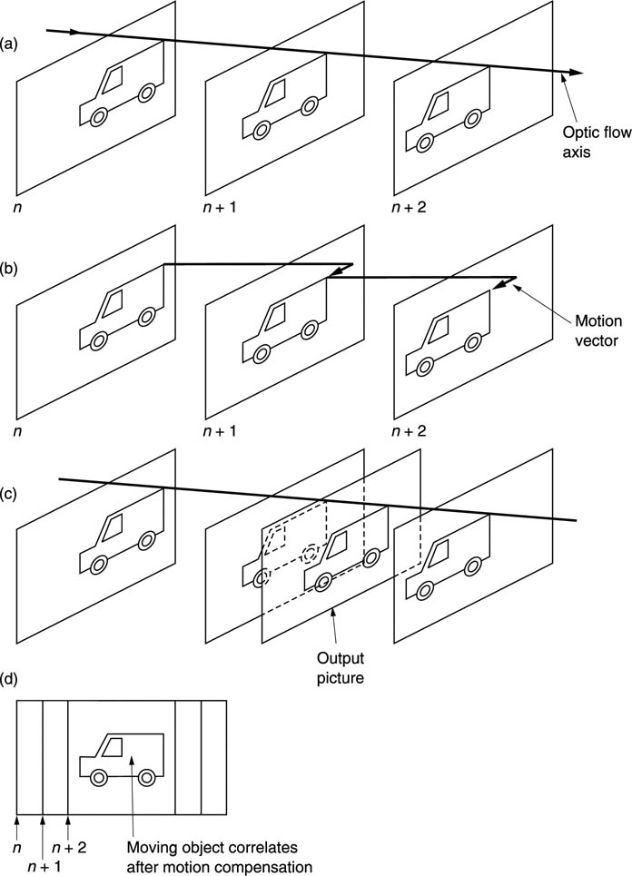
Figure 4.29(c) shows that if a high-quality standards conversion is required between two different frame rates, the output frames can be synthesized by moving image data, not through time, but along the optic flow axis. This locates objects where they would have been if frames had been sensed at those times, and the result is a judder-free conversion. This process can be extended to drive image displays at a frame rate higher than the input rate so that flicker and background strobing are reduced. This technology is available in certain high-quality consumer television sets. This approach may also be used with 24 Hz film to eliminate judder in telecine machines.
Figure 4.29(d) shows that noise reduction relies on averaging two or more images so that the images add but the noise cancels. Conventional noise reducers fail in the presence of motion, but if the averaging process takes place along the optic flow axis, noise reduction can continue to operate.
The way in which eye tracking avoids aliasing is fundamental to the perceived quality of television pictures. Many processes need to manipulate moving images in the same way in order to avoid the obvious difficulty of processing with respect to a fixed frame of reference. Processes of this kind are referred to as motion compensated and rely on a quite separate process which has measured the motion. Motion compensation is also important where interlaced video needs to be processed as it allows the best possible de-interlacing performance.
4.6 Motion-compensated standards conversion
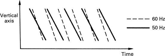
A conventional standards convertor is not transparent to motion portrayal, and the effect is judder and loss of resolution. Figure 4.30 shows what happens on the time axis in a conversion between 60 Hz and 50 Hz (in either direction). Fields in the two standards appear in different planes cutting through the spatiotemporal volume, and the job of the standards convertor is to interpolate along the time axis between input planes in one standard in order to estimate what an intermediate plane in the other standard would look like. With still images, this is easy, because planes can be slid up and down the time axis with no ill effect. If an object is moving, it will be in a different place in successive fields. Interpolating between several fields results in multiple images of the object. The position of the dominant image will not move smoothly, an effect which is perceived as judder. Motion compensation is designed to eliminate this undesirable judder.
Figure 4.30 The different temporal distribution of input and output fields in a 50/60 Hz convertor.
A conventional standards convertor interpolates only along the time axis, whereas a motion-compensated standards convertor can swivel its interpolation axis off the time axis. Figure 4.31(a) shows the input fields in which three objects are moving in a different way. At (b) it will be seen that the interpolation axis is aligned with the optic flow axis of each moving object in turn.
Figure 4.31 (a) Input fields with moving objects. (b) Moving the interpolation axes to make them parallel to the trajectory of each object.

Each object is no longer moving with respect to its own optic flow axis, and so on that axis it no longer generates temporal frequencies due to motion and temporal aliasing due to motion cannot occur.5 Interpolation along the optic flow axes will then result in a sequence of output fields in which motion is properly portrayed. The process requires a standards convertor which contains filters that are modified to allow the interpolation axis to move dynamically within each output field. The signals which move the interpolation axis are known as motion vectors. It is the job of the motion-estimation system to provide these motion vectors. The overall performance of the convertor is determined primarily by the accuracy of the motion vectors. An incorrect vector will result in unrelated pixels from several fields being superimposed and the result is unsatisfactory.
Figure 4.32 shows the sequence of events in a motion-compensated standards convertor. The motion estimator measures movements between successive fields. These motions must then be attributed to objects by creating boundaries around sets of pixels having the same motion. The result of this process is a set of motion vectors, hence the term ‘vector assignation’. The motion vectors are then input to a modified four-field standards convertor in order to deflect the inter-field interpolation axis.
Figure 4.32 The essential stages of a motion-compensated standards convertor.

The vectors from the motion estimator actually measure the distance moved by an object from one input field to another. What the standards convertor requires is the value of motion vectors at an output field. A vector interpolation stage is required which computes where between the input fields A and B the current output field lies, and uses this to proportion the motion vector into two parts. Figure 4.33(a) shows that the first part is the motion between field A and the output field; the second is the motion between field B and the output field. Clearly, the difference between these two vectors is the motion between input fields. These processed vectors are used to displace parts of the input fields so that the axis of interpolation lies along the optic flow axis. The moving object is stationary with respect to this axis so interpolation between fields along it will not result in any judder.
Figure 4.33 The motion vectors on the input field structure must be interpolated onto the output field structure as in (a). The field to be interpolated is positioned temporally between source fields and the motion vector between them is apportioned according to the location. Motion vectors are two dimensional, and can be transmitted as vertical and horizontal components shown at (b) which control the spatial shifting of input fields.
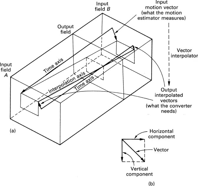
Whilst a conventional convertor only needs to interpolate vertically and temporally, a motion-compensated convertor also needs to interpolate horizontally to account for lateral movement in images. Figure 4.33(b) shows that the motion vector from the motion estimator is resolved into two components, vertical and horizontal. The spatial impulse response of the interpolator is shifted in two dimensions by these components. This shift may be different in each of the fields which contribute to the output field.
When an object in the picture moves, it will obscure its background. The vector interpolator in the standards convertor handles this automatically provided the motion estimation has produced correct vectors. Figure 4.34 shows an example of background handling. The moving object produces a finite vector associated with each pixel, whereas the stationary background produces zero vectors except in the area O–X where the background is being obscured. Vectors converge in the area where the background is being obscured, and diverge where it is being revealed. Image correlation is poor in these areas so no valid vector is assigned.
Figure 4.34 Background handling. When a vector for an output pixel near a moving object is not known, the vectors from adjacent background areas are assumed. Converging vectors imply obscuring is taking place which requires that interpolation can only use previous field data. Diverging vectors imply that the background is being revealed and interpolation can only use data from later fields.

An output field is located between input fields, and vectors are projected through it to locate the intermediate position of moving objects. These are interpolated along an axis which is parallel to the optic flow axis. This results in address mapping which locates the moving object in the input field RAMs. However, the background is not moving and so the optic flow axis is parallel to the time axis. The pixel immediately below the leading edge of the moving object does not have a valid vector because it is in the area O-X where forward image correlation failed.
The solution is for that pixel to assume the motion vector of the background below point X, but only to interpolate in a backwards direction, taking pixel data from previous fields. In a similar way, the pixel immediately behind the trailing edge takes the motion vector for the background above point Y and interpolates only in a forward direction, taking pixel data from future fields. The result is that the moving object is portrayed in the correct place on its trajectory, and the background around it is filled in only from fields which contain useful data.
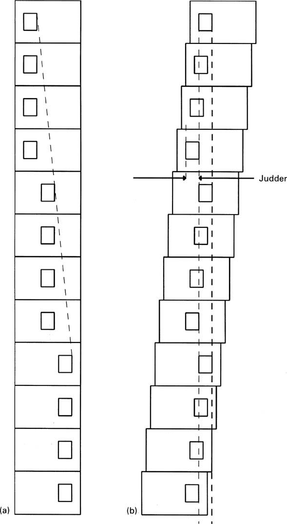
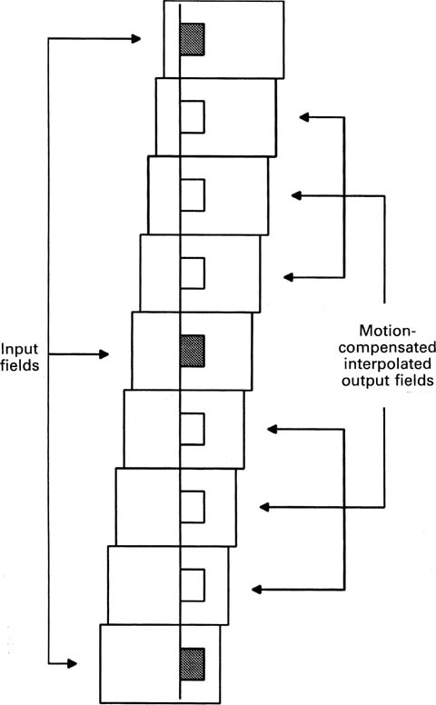
The technology of the motion-compensated standards convertor can be used in other applications. When video recordings are played back in slow motion, the result is that the same picture is displayed several times, followed by a jump to the next picture. Figure 4.35 shows that a moving object would remain in the same place on the screen during picture repeats, but jump to a new position as a new picture was played. The eye attempts to track the moving object, but, as Figure 4.35 also shows, the location of the moving object wanders with respect to the trajectory of the eye, and this is visible as judder.
Figure 4.35 Conventional slow motion using field repeating with stationary eye shown at (a). With tracking eye at (b) the source of judder is seen.
Motion-compensated slow-motion systems are capable of synthesizing new images which lie between the original images from a slow-motion source. Figure 4.36 shows that two successive images in the original recording (using DVE terminology, these are source fields) are fed into the unit, which then measures the distance travelled by all moving objects between those images. Using interpolation, intermediate fields (target fields) are computed in which moving objects are positioned so that they lie on the eye trajectory. Using the principles described above, background information is removed as moving objects conceal it, and replaced as the rear of an object reveals it. Judder is thus removed and motion with a fluid quality is obtained.
Figure 4.36 In motion-compensated slow motion, output fields are interpolated with moving objects displaying judder-free linear motion between input fields.
4.7 De-interlacing
Interlace is a compression technique which sends only half of the picture lines in each field. Whilst this works reasonably well for transmission, it causes difficulty in any process which requires image manipulation. This includes DVEs, standards convertors and display convertors. All these devices give better results when working with progressively scanned data and if the source material is interlaced, a de-interlacing process will be necessary.
Interlace distributes vertical detail information over two fields and for maximum resolution all that information is necessary. Unfortunately it is not possible to use the information from two different fields directly. Figure 4.37 shows a scene in which an object is moving. When the second field of the scene leaves the camera, the object will have assumed a different position from the one it had in the first field, and the result of combining the two fields to make a de-interlaced frame will be a double image. This effect can easily be demonstrated on any video recorder which offers a choice of still field or still frame. Stationary objects before a stationary camera, however, can be de-interlaced perfectly.
Figure 4.37 Moving object will be in a different place in two successive fields and will produce a double image.

In simple de-interlacers, motion sensing is used so that de-interlacing can be disabled when movement occurs, and interpolation from a single field is used instead. Motion sensing implies comparison of one picture with the next. If interpolation is only to be used in areas where there is movement, it is necessary to test for motion over the entire frame. Motion can be simply detected by comparing the luminance value of a given pixel with the value of the same pixel two fields earlier. As two fields are to be combined, and motion can occur in either, then the comparison must be made between two odd fields and two even fields. Thus four fields of memory are needed to correctly perform motion sensing. The luminance from four fields requires about a megabyte of storage.
At some point a decision must be made to abandon pixels from the previous field which are in the wrong place due to motion, and to interpolate them from adjacent lines in the current field. Switching suddenly in this way is visible, and there is a more sophisticated mechanism which can be used. In Figure 4.38, two fields are shown, separated in time. Interlace can be seen by following lines from pixels in one field, which pass between pixels in the other field. If there is no movement, the fact that the two fields are separated in time is irrelevant, and the two can be superimposed to make a frame array. When there is motion, pixels from above and below the unknown pixels are added together and divided by two, to produce interpolated values. If both of these mechanisms work all the time, a better quality picture results if a crossfade is made between the two based on the amount of motion. A suitable digital crossfader was shown in section 4.1. At some motion value, or some magnitude of pixel difference, the loss of resolution due to a double image is equal to the loss of resolution due to interpolation. That amount of motion should result in the crossfader arriving at a 50/50 setting. Any less motion will result in a fade towards both fields, any more motion in a fade towards the interpolated values.
Figure 4.38 Pixels from the most recent field (·) are interpolated spatially to form low vertical resolution pixels (x) which will be used if there is excessive motion; pixels from the previous field (□) will be used to give maximum vertical resolution. The best possible de-interlaced frame results.

The most efficient way of de-interlacing is to use motion compensation. Figure 4.39 shows that when an object moves in an interlaced system, the interlace breaks down with respect to the optic flow axis as was seen in section 2.11. If the motion is known, two or more fields can be shifted so that a moving object is in the same place in both. Pixels from both field can then be used to describe the object with better resolution than would be possible from one field alone. It will be seen from Figure 4.40 that the combination of two fields in this way will result in pixels having a highly irregular spacing and a special type of filter is needed to convert this back to a progressive frame with regular pixel spacing. At some critical vertical speeds there will be alignment between pixels in adjacent fields and no improvement is possible, but at other speeds the process will always give better results.
Figure 4.39 In the presence of vertical motion or motion having a vertical component, interlace breaks down and the pixel spacing with respect to the tracking eye becomes irregular.
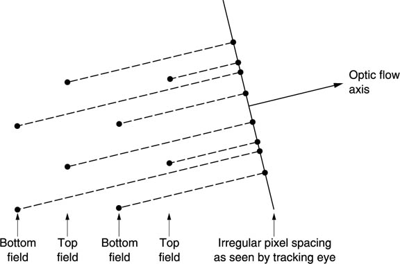
Figure 4.40 A de-interlacer needs an interpolator which can operate with input samples which are positioned arbitrarily rather than regularly.

4.8 Noise reduction
The basic principle of all video noise reducers is that there is a certain amount of correlation between the video content of successive frames, whereas there is no correlation between the noise content.
A basic recursive device is shown in Figure 4.41. There is a frame store which acts as a delay, and the output of the delay can be fed back to the input through an attenuator, which in the digital domain will be a multiplier. In the case of a still picture, successive frames will be identical, and the recursion will be large. This means that the output video will actually be the average of many frames. If there is movement of the image, it will be necessary to reduce the amount of recursion to prevent the generation of trails or smears. Probably the most famous examples of recursion smear are the television pictures sent back of astronauts walking on the moon. The received pictures were very noisy and needed a lot of averaging to make them viewable. This was fine until the astronaut moved. The technology of the day did not permit motion sensing.
Figure 4.41 A basic recursive device feeds back the output to the input via a frame store which acts as a delay. The characteristics of the device are controlled totally by the values of the two coefficients K1 and K2 which control the multipliers.

The noise reduction increases with the number of frames over which the noise is integrated, but image motion prevents simple combining of frames. If motion estimation is available, the image of a moving object in a particular frame can be integrated from the images in several frames which have been superimposed on the same part of the screen by displacements derived from the motion measurement. The result is that greater reduction of noise becomes possible.6 In fact a motion-compensated standards convertor performs such a noise reduction process automatically and can be used as a noise reducer, albeit an expensive one, by setting both input and output to the same standard.
References
1. Newman, W.M. and Sproull, R.F., Principles of Interactive Computer graphics, Tokyo: McGraw-Hill (1979)
2. Gernsheim, H., A Concise History of Photography, London: Thames and Hudson, 9–15 (1971)
3. Hedgecoe, J., The Photographer’s Handbook, London: Ebury Press, 104–105 (1977)
4. 4de Boor, C., A Practical Guide to Splines, Berlin: Springer (1978)
5. Lau, H. and Lyon, D. Motion compensated processing for enhanced slow motion and standards conversion. IEE Conf. Publ. No. 358, 62–66 (1992)
6. Weiss, P. and Christensson, J., Real time implementation of sub-pixel motion estimation for broadcast applications. IEE Digest, 1990/128