CHAPTER 27

Trading and Investment Strategies in Behavioral Finance

John M. Longo, CFA

Clinical Professor of Finance and Economics, Rutgers Business School—Newark and New Brunswick, and Chief Investment Officer, The MDE Group, Inc.

INTRODUCTION

Behavioral finance was once on the fringe of academic finance, but now it clearly has wide acceptance with investment professionals and individual investors. Although behavioral finance is not a new concept, it has garnered increasing attention and respect in recent years. Keynes (1936) understood the role of investor psychology in markets when he indicated that “animal spirits” drove prices. According to Benjamin Graham (1973, p. xv), the father of value investing, “The investor's chief problem—and even his worst enemy—is likely to be himself.” The ultimate imprimatur occurred in 2002, when Daniel Kahneman and Vernon Smith received the Nobel Memorial Prize in Economic Sciences for their work in behavioral finance and experimental economics. Thaler (1999), a leading scholar in the field, predicts that the term “behavioral finance” will be a redundant term, noting, “What other kind of finance is there?”

This chapter focuses on questions related to the practical analysis and understanding of behavioral finance. For example, what investment strategies associated with behavioral finance have been at least partially successful? What excess returns have these strategies historically generated? Are these strategies likely to continue to add value? How are investment funds attempting to capitalize on behavioral biases? What are some current and future trends in behavioral finance?

The remainder of this chapter has the following organization. The first section examines the distinction between trading and investment strategies. Next, the chapter analyzes how active versus passive strategies fit into a behavioral finance framework. The subsequent section documents evidence that average investors suffer from behavioral biases that negatively affect their performance. The chapter next analyzes a range of short-term trading approaches and then long-term investment oriented strategies grounded in behavioral finance. The next section discusses current and future trends in behavioral based strategies. Lastly, the chapter summarizes its findings and concludes.

DISTINCTION BETWEEN TRADING AND INVESTMENT STRATEGIES

From an analytical perspective, behavioral biases can occur within a short-term trading strategy or long-term investment time horizon. Graham and Dodd (1934, p. 16) distinguish between short-term speculation and long-term investment as follows: “An investment operation is one which, upon thorough analysis promises safety of principal and an adequate return. Operations not meeting the requirements are speculative.”

Although Graham and Dodd's definition makes intuitive sense, it lacks clear points of demarcation from an organizational perspective. This chapter describes investment strategies as those with investment horizons generally greater than one year. For example, the reversal effect pioneered by DeBondt and Thaler (1985) where long-term winners (losers) subsequently underperform (outperform) is an example of an investment strategy according to Graham and Dodd's definition.

Conversely, trading strategies have investment horizons less than one year and as short as a millisecond. The momentum effect, popularized by Jegadeesh and Titman (1993), would fall under this definition of a trading strategy. The momentum effect is the tendency for rising equity prices to rise further and falling equity prices to keep falling. In general, trading strategies are more germane to the ultracompetitive hedge fund industry, while investment strategies are more suitable for the typical mutual fund, pension fund, or individual investors. Of course, exceptions exist, but the one-year investment horizon demarcation point provides some clarity from a testing perspective. Lastly, the tax authorities in many countries (e.g., Internal Revenue Service in the United States) distinguish between short- and long-term security holdings. The latter horizon in general is taxed at a 15 to 20 percent capital gains rate in the United States, while the former is taxed at higher rates at or near the investors' marginal tax bracket. A provision of the Obamacare legislation resulted in an additional 3.8 percent tax on investment income for wealthy individuals.

ACTIVE VERSUS PASSIVE INVESTMENT STRATEGIES AND BEHAVIORAL FINANCE

Behavioral finance adherents generally fall into the active management camp because they often believe that behavioral biases are systematic and exploitable in nature, at least from a social science perspective. In other words, the law of gravity or quantum mechanics in the physical sciences is likely to hold true almost 100 percent of the time. However, in the social sciences, a model that provides, for example, 55 percent accuracy is likely to add substantial value over the long term. A simple way of assessing the value in a model that has modest predictive ability, relative to one that is purely random, is to consider what would happen if someone won 55 percent of the time when betting on black in a game of roulette. Certainly, any individual spin of the roulette wheel may result in a loss, namely, red or green in this example. However, the individual makes enough of these small bets to have a very successful financial outcome over time.

Reviewing some simple arithmetic may be helpful in seeing the difficulty of outperforming a passive benchmark. Sharpe (1991) demonstrates that the average investor cannot outperform the average return on an investment when including transaction costs. That is, the person will underperform. Although professional fund managers (i.e., sharks, smart money, or informed investors) should be able to take advantage of retail investors (i.e., dumb money or uninformed investors), empirical evidence does not support this notion. In fact, the evidence typically shows that professional fund managers cannot consistently outperform a market index, such as the S&P 500, on a risk-adjusted basis. For example, Bodie, Kane, and Marcus (2010) show the performance of the average equity mutual fund versus the Wilshire 5000 equity index. Consistent with Sharpe's theoretical results, their results indicate that professional fund managers modestly underperform the benchmark.

Investors' risk tolerance may also affect their asset allocation strategies. For example, most investors do not make yearly adjustments to retirement accounts because they suffer from status quo bias (Kahneman, Knetsch, and Thaler 1991). Status quo bias refers to an irrational preference for the current state of affairs. The status quo or current investment posture is taken as a reference point. Any change from the initial reference point is perceived as a loss.

Several approaches may be beneficial to investors in order to overcome the status quo biases. The first approach is to use automatic rebalancing in a 401(k) plan, such as reverting to a 60 percent equity and 40 percent fixed income portfolio on January 1 of each year or a person's birthday. Active asset allocation is a second approach to overcoming the status quo bias because it forces active decision-making on the part of investors or their advisors. Lastly, a life cycle fund engages in active asset allocation, typically becoming more conservative as a specific target date approaches, such as a planned retirement date.

Yet, a glimmer of hope exists for advocates of active management. Several studies such as Malkiel (1995) and Bollen and Busse (2005) find modest evidence showing persistent performance. That is, winning (losing) managers, on balance, keep on winning (losing). For example, the investment performance of Warren Buffett, Peter Lynch, James Simons, George Soros, and other members of the proverbial investment hall of fame provide support for the persistence theory, while the overall distribution of outperformers remains consistent with market efficiency.

If markets are not fully efficient, active management may be a worthwhile activity for those willing to put substantial amounts of time and rigorous effort into the endeavor. However, any active manager should have a healthy respect for both the difficulty in outperforming an index on a risk-adjusted basis and in overcoming (broadly defined) transaction costs. Investors who lack a passion for the financial markets or access to highly knowledgeable and experienced financial advisors are likely best served with index funds. Vanguard and Dimensional Fund Advisors (DFA) have both built phenomenally successful businesses using index funds as their primary investment approach. This chapter is mainly designed for those who believe in active management and want to improve their investment performance by capitalizing on knowledge from behavioral finance.

Currently, many successful investment firms base their investment decisions on behavioral finance principles. For example, LSV Asset Management, a firm formed by three academic “stars” of behavioral finance research, has about $65 billion under management. The “Investment Philosophy” section of the LSV's website states, “The fundamental premise on which our investment philosophy is based is that superior long-term results can be achieved by systematically exploiting the judgmental biases and behavioral weaknesses that influence the decisions of many investors” (LSV Asset Management 2013). Fuller and Thaler Asset Management have trademarked the term “The Behavioral Edge®” to succinctly describe their strategy. This firm's home page states, “Investors make mental mistakes that can cause stocks to be mispriced. Fuller & Thaler's objective is to use our understanding of human decision-making to find these mispriced stocks and earn superior returns” (Fuller and Thaler Asset Management 2013).

AVERAGE INVESTORS SUFFER FROM BEHAVIORAL BIASES

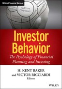
The old adage that a picture is worth a thousand words likely applies to Exhibit 27.1. The exhibit shows that the average investor in equity funds over the 15-year period from 1998 through 2012 averaged returns less than half those earned by the S&P 500 Index. Even after taking into account (actively managed fund) fees and transaction costs, the average investor clearly underperformed during this period. What is probably driving this result is the behavioral bias of “chasing” investment performance. That is, the typical investor buys what has done well recently and, on the downside, often sells near the market lows. Although the success of following momentum strategies is discussed throughout this chapter, investors are typically not nimble enough in their investment decisions to profit from the momentum anomaly. They often buy an asset after it has risen substantially in price, perhaps due to media attention given to these “star” investments. Inevitably, a loss occurs. If the loss is severe, a “capitulation” event often occurs, where the investor sells near a bottom.

The investment implications of the Exhibit 27.1 are perhaps twofold. A portfolio of index funds may best serve investors with long-term horizons so they do not succumb to the performance chasing bias. Investors using an active management approach should exercise extreme caution in their entry and exit points. In some instances, following a dollar cost averaging approach may be a better course of action. For the active trader, the momentum anomaly likely works in the short run—for example, buy (short) what has worked well (poorly) recently, but be poised to exit the investment if the market cycle changes.

PROBLEMS WITH TRADITIONAL INVESTMENT STRATEGIES

Many widely accepted academic theories of traditional finance and practitioner investment strategies fall short of their promises when implemented over a full market cycle. This section examines several strategies, such as those based on Markowtz (1952, 1959) portfolio theory, the dividend discount model (DDM), hedge funds, and the endowment model, and discusses where each falls short of performance expectations in practice. The inability of these approaches to effectively describe financial reality creates an opening for behaviorally based investment strategies, which is the focus of the following section.

Problems with Markowitz Portfolio Theory

Markowitz (1952, 1959), who shared the 1990 Nobel Memorial Prize in Economic Sciences, provides one of the seminal contributions to finance. He was the first to explicitly measure portfolio risk and fully understood the impact of correlation on the risk of the portfolio, rather than merely the risk of the underlying securities. Markowitz also developed a quadratic program, a substantial mathematical achievement, to solve for what he termed as efficient portfolios (i.e., the investment opportunity set that maximizes return for a given level of risk or minimizes risk for a given level of return).

Although many still use Markowitz portfolio theory at the asset allocation level, its practicality has limitations at the individual stock selection level for most investor applications. First, the efficient frontier is unstable. In other words, a recommended portfolio for an investor today may differ markedly from a new optimization for the same investor at a later date. Financial advisors would lose credibility with their clients by recommending major portfolio adjustments on such a frequent basis. Second, the practical application of the Markowitz model, like nearly all models, is based on the quality of its inputs, such as the expected return and risk as measured by the standard deviation of each security. The most common methods for obtaining estimates all have flaws, such as the capital asset pricing model (CAPM), market model, arbitrage pricing theory (APT), and Fama-French three-factor model. Third, an important flaw with practical applications of the Markowitz model is that correlations often increase close to a perfect positive correlation (+1) during times of economic distress, thus eliminating the benefit of diversification, which is a central assumption of the model. Therefore, the investment principle of diversification often does not provide meaningful help precisely when investors need it most.

Problems with Dividend Discount Model

The dividend discount model (DDM) basically states that the price of a stock (or other asset) equals the present value of the future cash flows generated by the asset. Theoretically, its logic is unassailable. Investors know that “time is money” and that they should discount future cash flows back to the present. Yet, applying the model in the real world reveals its shortcomings. Although valuing an asset as the present value of future cash flows works well for bonds, it remains a challenging task for stocks that exist in perpetuity. How can an analyst reliably predict dividends or earnings for a firm out one year, let alone in perpetuity?

The DDM has three major forms: no growth, constant growth, and irregular growth. Let's look at the constant growth version of the model, often called the Gordon constant growth model, because of its wide use in finance textbooks and the Chartered Financial Analysts (CFA) program. Its equation is as follows:

(27.1)

where P0 is today's price estimate; D1 is the estimate of next year's dividend (or free cash flow); r is the discount rate or cost of equity capital estimate; and g is the estimate of the terminal or constant growth rate of dividends (or free cash flow).

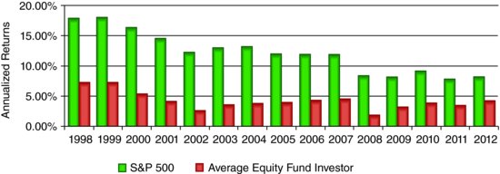
Assume that an investor can estimate each of the variables on the right-hand side of Equation 27.1 with a reasonable degree of precision. A simple numerical example illustrates some practical difficulties of the DDM, despite its theoretical elegance. Assume a base case that next year's dividend (or free cash flow) is $1 per share, the discount rate is 12 percent, and the constant growth rate is 3 percent. Investors often conduct a sensitivity analysis by varying the discount rate and growth rate. Varying the projected dividend next year is possible, but they make this adjustment less often.

Exhibit 27.2 shows the results for a range of discount rates and growth factors. Making relatively minor changes in the inputs results in a large variation in the price. Under the base case assumptions, the stock price is $11.11. Using a more optimistic scenario with a 10 percent discount rate and 5 percent growth rate results in a price of $20.00. This is a difference of 80 percent from the base case. Using a more pessimistic scenario of a 14 percent discount rate and a 1 percent growth rate results in a price of $7.69, representing a 31 percent drop from the base case. The range of reasonable estimates (e.g., $7.69 to $20.00) is so wide it often makes the DDM of limited use to professional fund managers. In essence, an investor can justify almost any valuation by changing the inputs.

Although the DDM can add some value, especially for dividend-paying stocks in the mature stage of their life cycle, analysts and investors should be wary of using it as a primary valuation technique. The DDM may also provide a valuable reality check during anomalous periods of overreaction, on both the upside and downside, in the market. Using the DDM as a reality check against the prices of technology stocks during times such as the Internet bubble period of the late 1990s through early 2000 may have added substantial value. Almost any application of the DDM to technology stocks would have indicated huge overvaluation. For example, the stock price performance of Microstrategy, a business intelligence software maker, provides one dramatic example of the irrationality that occurred during this period. Microstrategy went from roughly $25 per share shortly after its initial public offering (IPO) in mid-1998 to a breathtaking $3,500 a share at the peak of the Internet bubble in March 2000. The stock ultimately crashed to $4 a share and rebounded to $108 in March 2013, still down almost 97 percent from its peak.

Problems with Hedge Funds and Endowment Model

In the 2000–2002 aftermath of the Internet bubble, hedge funds were highly popular in the investment world. Hedge funds are private investment vehicles sold to high net worth investors or institutions. The average hedge fund provided modestly positive returns during each of these calendar years, while most equity indexes plunged double digits and lost more than half their value on a peak-to-trough basis. Although hedge fund assets increased more than tenfold from 2000 to 2012, the illusion of hedge fund invincibility was dispelled in 2008 when the average hedge fund lost 23.25 percent, according to the Hedge Fund Research (HFRX) Index. A similar and somewhat more surprising breakdown occurred in 2011 when the HFRX Index lost 8.87 percent compared to modestly positive S&P 500 performance (Eder 2011).

In light of these disappointments, investment managers and their constituencies alike were dismayed to learn that many hedge funds—despite their name—had no material “hedge” or risk reduction features. More recently, the term “hedge fund” has evolved to refer simply to an investment within a partnership structure that has the ability to charge incentive fees. The last decade has not been a good one for hedge fund performance. Somewhat ironically, 2008 was the best year of relative performance for hedge funds over the last 10 years in comparison to the S&P 500. But for the full decade, hedge funds, as measured by the HFRX index, underperformed inflation according to an analysis performed by The Economist (2012). That analysis further shows that hedge funds underperformed a simple 60 percent/40 percent equity bond index during the same period by an astounding margin. That is, the equity bond index returned 90 percent while the HFRX Hedge Fund Index was up only 17 percent.

What hedge fund investors often overlook is that these vehicles must achieve huge gross returns in order to deliver merely adequate net returns to the client. This is an important issue in recent years in an environment of high correlations, low yields, and limited returns. To understand why this is the case, consider an investment in a typical hedge fund. To be conservative, assume that the underlying individual hedge fund charges fees of 1.5 percent of assets and 20 percent of profits. In fact, many hedge funds charge 2 percent of assets plus 20 percent of profits. Also assume an annual expense ratio of 0.5 percent for the hedge fund partnership structure and that the individual hedge fund pays 2 percent in annual transaction costs.

Exhibit 27.3 shows that the net returns to an investor are startling. A seemingly impressive 14.0 percent gross return shrinks to a far more modest 8.0 percent net return after paying fees and expenses. A fund of funds structure may exacerbate the problem because it may require that underlying managers produce nearly a 17.0 percent gross return to net 8 percent to the end investor. As the name suggests, a fund of funds is a hedge fund that holds positions in underlying individual hedge funds. This extra return is necessary to cover the additional layer of partnership expenses as well as a typical fee structure of 1 percent of assets plus 10 percent of the profits in a fund of funds structure.

Exhibit 27.3 Hedge Fund Gross versus Net Returns

Calculation of Net Return to Investor	%
Hypothetical gross return of fund	14.0
Hedge fund: transaction costs	−2.0
Hedge fund: base fee	−1.5
Hedge fund: expenses	−0.5
Hedge fund: incentive fee (20%)	−2.0
Net return to investor	8.0
Note: Hedge funds are burdened with high investment fees and underlying expenses. In this example, a 14 percent gross return for the fund shrinks to an 8 percent net return for the investor.

The main lesson is not that hedge funds are expensive or have underperformed, but that they need to generate superior gross returns to deliver acceptable net returns to investors. This often causes hedge fund managers to stretch for returns, creating unrecognized and uncompensated risk as managers take above-market risks with investor capital to generate returns sufficient to cover their very substantial fees and underlying expenses. Additionally, limited hedge fund transparency often prevents investors from recognizing the added risk until they no longer have time to respond. Other hedge fund flaws also exact their toll. Lockup provisions, gates, or side pockets limit exit opportunities once added risk issues are uncovered. A lockup provision refers to the minimum holding period for a hedge fund, without incurring a substantial early exit fee. Gates on a hedge fund limit the ability to redeem from a hedge fund even after the lockup period expires. Gates are usually erected during times of substantial redemptions for a hedge fund. Side pockets refer to holdings in illiquid assets, such as private equity investments, that hedge fund investors hold after requesting redemption. Transparency not only plays a role in uncovering fraud or unacceptable risks, but it also helps investment managers better understand where a particular hedge fund fits within their portfolios.

A prodigy of the Markowitz model called the endowment model, popularized by David Swenson of Yale, added large positions in hedge funds, private equity, and other illiquid sophisticated investments in an attempt to enhance returns while reducing risk. The focus on leveraged, illiquid, and alternative investments differentiates the endowment model from a traditional mix (e.g., 60 percent and 40 percent) of equity and debt, respectively. Despite attractive long-term performance, the endowment model failed during the financial crisis of 2007–2008 with many of its adherents losing in excess of 25 percent of invested capital.

Endowment funds are investment funds set up by nonprofit institutions to help finance their activities and long-term strategic plans. The endowment funds of some of the most prestigious American universities experienced substantial losses during the recent financial crisis. For example, during the fiscal year 2009 (July 1, 2008 through June 30, 2009), endowment performance for the following institutions dropped dramatically: Harvard (−27.3 percent), Stanford (−25.9 percent), Yale (−24.9 percent), and Princeton (−22.7 percent). The typical investor cannot replicate the investment opportunity set afforded to Yale and other large endowments.

In short, problems with existing models used by institutional and some retail investors provide opportunities for behaviorally based strategies with the objective of profiting from the mistakes of the “crowd.” Behavioral models are also likely to better explain how the markets work. The next section of this chapter focuses on these short-term strategies.

SHORT-TERM BEHAVIORALLY BASED TRADING STRATEGIES

The prior section established some of the problems with traditional financial theories and techniques used by practitioners. Fortunately, the behavioral finance literature provides some guidance into strategies that appear to consistently generate superior risk-adjusted returns. This section focuses on trading-oriented behavioral strategies that generally have a holding period of less than one year. These strategies are fallible and do not have the theoretical elegance of Markowitz portfolio theory or the CAPM, but are of practical value to professional investors. The behavioral finance literature suggests that these biases are unlikely to disappear quickly, raising the prospect of market-beating strategies.

Momentum

The success of momentum strategies is one of the most serious challenges to the efficient market hypothesis (EMH). The EMH states that security prices reflect all available information. Hence, consistently beating the market by devising an investment strategy that regularly delivers superior risk-adjusted returns is impossible. A common catchphrase among technical analysts for momentum is that “the trend is your friend.” In other words, winning investments keep winning, while losing investments keep losing, at least in relation to a market index. Momentum can be measured in many ways, but its calculation typically examines the price of an asset relative to an index. The relative strength and moving average statistics are among the most common statistics used to measure momentum. These metrics are computed below:

(27.2)

where Rx is the return of a stock or other asset over the specified time period and Ri is the return of an appropriate index or benchmark over the specified time period. Analysts sometimes normalize the relative strength figure into a relative strength index (RSI) with a value between 0 and 100. A number close to zero indicates that the security has experienced the worst performance versus its peers in the index over the specified time period, while a number closer to 100 signifies the best relative performance.

The short-term behavior of variables, such as stock prices, often shows a jagged, erratic pattern. Technicians often use a moving average to smooth out this volatile pattern in order to make judgments that do not flip-flop from buy to sell ratings too often. Moving averages can vary by length and they are typically analyzed in pairs. For example, a short-term trader may focus on the 5-day moving average relative to its 20-day moving average. Investors with longer horizons often focus on the 50-day moving average relative to the 200-day moving average. In both instances, if the shorter-term moving average is higher than the longer-term moving average, technical analysts generally view the investment as having relative strength. In this case, the relative strength is with respect to recent values of the investment, rather than performance versus an index.

(27.3)

where

P1 = the closing price of the asset on period (e.g., day) 1

P2 = the closing price of the asset on period (e.g., day) 2

PN = the closing price of the asset on period (e.g., day) N

N = the number of observations.

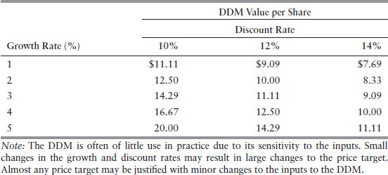
The calculation in Equation 27.3 is a simple moving average or just a moving average. Technicians often compute variations of the simple moving average, such as an exponentially weighted moving average, to put more weight on recent price movements. Exhibit 27.4 shows the 50-day versus 200-day moving average for Google in late May, 2013. The chart is bullish because the short-term moving average is higher than the longer-term moving average, and therefore indicative of positive price momentum.

Jegadeesh and Titman (1993) find that the momentum earns abnormal returns of roughly 1 percent per month for periods up to 12 months, but that the effect is the strongest in the three- to six-month range. Momentum is likely to add value because this approach is based on the central tenets of behavioral finance. Investors often mimic the behavior of other investors. If an individual observes another making large profits buying Amazon.com stock, the individual may follow suit. Momentum may also add investment value due to the way news makes its way into stock prices. In some instances, investors provide news to reporters and therefore legally trade on news before it is published. Unfortunately, in some circumstances, investors illegally trade on insider information and leave “footprints” in the price action of security prices. Other investors may infer that this abnormal buying causes prices to increase or decrease further.

Margin calls may also play a role in momentum. A margin call is a demand by a brokerage firm to deposit cash or securities in a financial account to provide collateral for recently experienced losses. A losing investment on the long side may result in the mandatory sale of securities, depressing prices further. Similarly, a losing investment on a short sale position may result in a “short squeeze” causing an additional increase in prices. A short squeeze is a request from a brokerage firm to an investor to cover a short sale position, which often results in a sharp increase in the price of the covered stock. Lastly, successful fund managers often receive cash inflows. In many instances they buy (short-sell) their existing holdings, pushing prices higher (lower).

Earnings Surprises

An earnings surprise is the difference between the reported earnings per share (EPS) (i.e., the actual EPS) and the consensus sell-side estimate (i.e., the estimated EPS), tracked by First Call, or another sell-side earnings aggregator. The surprise is positive if the reported EPS is greater than the consensus EPS estimate. Conversely, the surprise is negative if the company reports a number less than the consensus. Analysts often normalize the earnings surprise figure as a percentage, as shown below:

(27.4)

Researchers often sort earnings surprises into deciles. For example, an early study by Rendleman, Jones, and Latané (1982) shows how stocks with the biggest earnings surprise in decile 10 outperform those in decile 9 and decile 8, and so forth. A “long only” strategy could simply purchase stocks in decile 10 and, according to the historical Rendleman et al. numbers, earn abnormal returns of roughly 8 percent in the three months after the earnings announcement. Hedge funds may have an interest in a long/short variant of the strategy, going long stocks in decile 10 and selling short stocks in decile 1. The spread between these deciles is roughly an astonishing 16 percent over three months, multiplied by any leverage used by the hedge fund, net of interest expense and transaction costs. More recent studies such as Jegadeesh and Livnat (2006) continue to support superior returns generated by firms reporting positive earnings surprises, albeit at somewhat reduced levels from the Rendleman et al. study.

Why do earnings surprises persist? Jegadeesh and Titman (1993) are likely the first researchers to document underreaction as a persistent bias. The underreaction bias suggests that for some firms, new information gradually makes its way into the current price of a security, rather than the instantaneous approach suggested by the EMH. Investors often perceive prior winning or “glamour,” stocks as remaining market leaders for an extended period. Conversely, previous losing stocks, or “dogs,” often need time for skeptical investors to believe that their prior disappointing performance has truly changed.

In contrast to the Jegadeesh and Titman (1993) approach on momentum in stock returns, Dreman and Berry (1995) discuss underreaction in the framework of analyst estimates and valuation metrics. In the context of earnings surprises, when news arises, investors are skeptical so they need time to accept that the news is real or sustainable. So, firms with positive earnings surprises get some benefit of good news. Conversely, the market penalizes firms with negative surprises, but perhaps not to the full extent that might be warranted. More elementary, buying and selling does not happen instantaneously. Some investors take time to process an earnings report and conduct appropriate follow-up research, thereby resulting in a delayed reaction. Lastly, good management knows how to use the slogan “under promise and over deliver.” Perhaps the management of firms with negative earnings surprises has not mastered this technique or operates in more volatile businesses that are not subject to the same earnings clarity. Tversky and Kahneman (1981) find that framing (i.e., adjusting the way that firms present earnings to investors) can sometimes fool investors and therefore may be another explanatory factor behind the persistence of the earning surprise anomaly.

Form 13F Filings and Hedge Fund Herding

The Securities and Exchange Commission (SEC) requires that all institutional investment managers with more than $100 million in assets under management report a portion of their holdings on a quarterly basis via Form 13F. Unfortunately, a fund does not have to disclose all holdings. For example, funds do not have to disclose short sale and some derivative positions but they must disclose long positions in stocks and options. Form 13F filings provide important information on the holdings of the portfolio of top portfolio managers, such as those managed by billionaire hedge fund managers. Professional investors widely follow these filings and seek to piggyback on the research and strong connections of the “star” managers. Does mimicking some of the trades reported in 13F filings pay? In a word, “Yes.” For example, Brav, Jiang, Partnoy, and Thomas (2008) find abnormal returns of 7 percent per year for activist hedge funds using Form 13F data.

Put/Call Ratio and Other Investor Sentiment Indicators

The term investor sentiment is synonymous with the terms feeling and emotion of investors. Clearly, these terms differ from purely rational behavior or the EMH. Analysts have created and historically applied several sentiment indicators to the market as a whole, but some may also be applicable to individual equities. This section discusses some investor sentiment indicators and the behavioral logic related to why they may be of value to investors.

Some attribute the put/call ratio indicator to investing legend Martin Zweig, who was best known for “calling” the Crash of 1987. Unlike most technical indicators that tend to be trend-following, the put/call ratio is a contrarian metric. Puts (sell) options enable investors to profit from a decline in the price of an asset and call (buy) options enable them to profit from a rise in a stock or other asset. A high value of the put/call ratio tends to indicate that investors are excessively bearish, hence perhaps the market may trend upward. Historically, more traders tend to buy call options then put options because the market goes up over the long term, so a value greater than 1 for the put/call ratio is uncommon. Many technicians view a value of the ratio as greater than 0.6 as bullish for equities. A behavioral connection to the put/call ratio is one of overreaction, or having the pendulum of market psychology move too far in one direction of price.

Arms (1996) devised the trading index (TRIN), which is sometimes called the Arms Index after its creator. Technicians generally believe that when a stock rises (falls) on high volume it is good (bad) news. Volume is the strength of the signal. If many stocks rise on high volume, this suggests a bullish signal. Conversely, if many stocks decline on high volume, TRIN provides a bearish omen. Equation 27.5 shows the TRIN calculation.

(27.5)

Because TRIN is a ratio of a ratio, its interpretation may be confusing. TRIN values less than 1 indicate bullish sentiment and strategy (i.e., many stocks are increasing on high relative volume to the decliners). Conversely, TRIN values greater than 1 are bearish. TRIN is consistent with the herding behavioral bias documented by Lakonishok, Shleifer, and Vishny (1992) as well as the euphoric (despair) feeling that often occurs in bull (bear) markets.

The Barron's confidence index is a ratio of the average yield-to-maturity of its best-grade bond list compared to the average yield-to-maturity of its intermediate grade bond list. Analysts often multiply this ratio by 100 to give a number more resembling that of a stock or index price. This index is roughly the equivalent of the ratio of AA or better bond yields to BBB bond yields. Because AAA bonds always sell at a lower yield to maturity than BBB bonds due to their lower credit risk, the index always trades at a value less than one. The Barron's confidence index examines the relative level of this ratio. Because values closer to one indicate a willingness to take on credit risk, they may be signs of an improving economy, a bullish stock market, and optimism bias. Optimism bias is the tendency to view one's own risk as less than that of others. Conversely, values well below one may indicate flight to quality or panic movements. Hence, low values would be bearish for stocks. Analysts consider index levels below 80 as bearish and values above 90 as bullish for stocks. In short, sentiment indicators attempt to measure the pulse or mood of the market and are therefore at the heart of behavioral biases of the market as a whole. The next section of this chapter focuses on long-term investment strategies.

LONG-TERM BEHAVIORALLY BASED INVESTMENT STRATEGIES

The behavioral finance literature documents several long-term investment strategies (i.e., those with holding periods greater than one year) that persistently generate superior risk-adjusted returns. This section focuses on several of these strategies, explaining their logic and the historical returns generated by the strategies. In the case of the Dogs of the Dow anomaly, an exchange traded fund (ETF) has been created to enable investors to simply and efficiently invest in the strategy.

Long-Term Price Reversals or Mean Reversion

The previous section discussed the shorter-term momentum effect in stock prices. That is, a strategy where winners (losers) kept winning (losing) for periods up to 18 months, but especially over a three-to-six month time frame. What about the momentum effect over the longer term? Researchers, such as DeBondt and Thaler (1985), find that over a three-to-five year period the reverse occurs. In others words, a basket of winners (losers) over the prior three to five years becomes losers (winners) over the next three to five years. DeBondt and Thaler report that the prior losers subsequently outperform the prior winners by 25 percent over a three-year period and with less risk.

Behavioral finance researchers view this finding as an overreaction effect in which investors tend to extrapolate trends over long periods. A basket of “star” stocks, despite the occasional IBM or Google, rarely can maintain its leadership position as a “hot stock” for an extended period. Some star stocks often attract intense competition or perhaps never deserved their star status. Conversely, a basket of stocks containing companies “left for dead” can often rebound despite some high profile stocks such as Enron, Kodak, and General Motors dropping dramatically.

Dogs of the Dow and Other Value Anomalies

Researchers such as Fama and French (1992) find that value stocks outperform growth stocks. However, investors suffer from behavioral bias that causes them to assume growth stocks have a better historical investment performance than value stocks most of the time. Of course, many ways are available to measure value, such as low price/earnings (P/E), low price-to-book (or its reciprocal book-to-market), low price-to-cash flow, and high dividend yield. The focus on a specific valuation metric is how this anomaly differs from the (price) momentum and reversal effects discussed earlier. The Dogs of the Dow strategy provides an intuitive example of the strategy in action and its possibly related behavioral bias. It focuses on the 10 highest dividend yielding stocks among the 30 stocks in the Dow Jones Industrial Average (DJIA). The strategy received widespread attention after the publication of Beating the Dow by Michael O'Higgins (1991). O'Higgins finds that the “dogs” strategy outperformed the (full) DJIA by about 3 percentage points a year.

Why may this strategy add value? Clearly, it is tied to the value anomaly, but the strategy may also be a variant of the “too big to fail” theme that analysts typically apply to banks. Although some former Dow stocks such as Kodak and General Motors fail, the vast majority are large, well capitalized, international companies. Jack Welch, legendary former chief executive officer of General Electric (GE) once noted that GE would be number one or two in each industry where it competes. If not, GE will fix or exit the business. Combining these thoughts suggests that although blue chip Dow companies may suffer from missteps, they can typically recover and shareholders will ultimately reward these stocks. A hefty dividend, with the strategy yielding 3.6 percent in April 2013, can help boost returns, especially when reinvesting dividends. ALPS Sector Dividend Dogs ETF (SDOG), an exchange traded fund (ETF), started in mid-2012 in an attempt to mimic the strategy.

Accruals Anomaly

Differences exist between earnings and cash flow. The former is an accounting construct, which is easy to manage; the latter shows the inflows and outflows of cash and is more difficult to manipulate. The reported earnings number relies on management choices of inventory valuation (e.g., last-in-first-out (LIFO) versus first-in-first-out (FIFO)), allowance for doubtful accounts, accounts payable, accounts receivable, and so forth. A “red flag” exists if a persistent difference occurs between earnings and cash flow over time, after adjusting for expected items such as depreciation, amortization, and changes in working capital.

Sloan (1996), who first identified the accruals anomaly, constructs a long/short portfolio with the long (short) portfolio consisting of firms with the least (most) accruals. He finds abnormal returns of roughly 10 percent a year for his long/short portfolio. Sloan suggests that the results are due to overreaction and cognitive errors as a result of Wall Street's fixation on earnings. This anomaly may also be a framing issue because management can apparently fool investors, at least some of the time, by putting the best spin on reported earnings. Currently, several ETFs such as the Forensic Accounting ETF (FLAG) use accounting quality of earnings filters, such as accruals.

CURRENT AND FUTURE TRENDS IN BEHAVIORAL FINANCE STRATEGIES

Overwhelming evidence suggests that the markets sometimes deviate from rationality. The EMH is “dead” in terms of the view that security prices always reflect all available information. However, alpha or persistent outperformance remains elusive. Alpha is a portfolio's actual return minus its expected return. The expected return is usually given from an asset pricing model such as the CAPM. Analysts and investors often deem portfolio managers with positive historical alphas as being successful, while those providing negative alphas may have less than secure job prospects.

Why is obtaining alpha in an investment strategy challenging despite a growing list of market anomalies? This occurs because humans are neither consistently rational nor irrational. Furthermore, the publication and widespread dissemination of an anomaly likely diminishes its effectiveness going forward. Hence, financial economists are unlikely to develop a unified CAPM type model that will neatly and simultaneously explain in a straightforward equation(s) both rational and irrational behavior. Hong and Stein (1999) have made perhaps the most valiant effort thus far to reconcile the various behavioral finance biases, such as momentum, underreaction, and overreaction.

Yet, hope remains for those who believe in active management. Documenting behavioral finance errors is somewhat akin to mapping the human genome. The current state of the art of personalized medicine is not that one can completely avoid disease, but that it might be detected earlier, making treatment more effective. Similarly, investors aware of the myriad of behavioral biases may be unable to completely avoid mistakes. Avoiding behavioral biases should be the minimum goal for any investor. The best case for the behavioral finance astute investor is to capitalize on the mistakes of others.

At least two areas are available for fruitful research in behavioral finance. The first is to analyze the wave of “big data” that is exploding across the Internet. Big data includes things such as Twitter feeds, Web-browsing behavior, video search, retail sales analysis, and data obtained from analog semiconductor devices. Analysis of big data may enable researchers to uncover emerging trends and hot products. Obviously, such a “black box” output would have important implications for picking investments. Some hedge fund managers are analyzing satellite images and Twitter data, looking for an investment edge.

A second fruitful area for research is combining or disentangling behavioral anomalies. For example, this chapter discusses the overreaction bias across diverse areas such as momentum, accruals, and reversals. Once again, using a medical analogy, having a holistic view of how biases interact, rather than focusing on one specific item, is important.

SUMMARY

Behavioral finance now has broad approval among financial practitioners. However, many in academic finance still are proponents of the traditional finance school. Investment professionals and individual investors argue that securities markets are inefficient in the context of prices and do not always reflect all available information. Clearly, achieving a positive alpha for a portfolio remains elusive for most managers, but findings of behavioral finance may provide important clues. Indeed, successful asset management firms, such as LSV Asset Management and Fuller and Thaler Asset Management, are thriving with findings from the behavioral finance field as the foundation for their strategies.

Important anomalies including momentum, accruals, value, reversals, earnings surprises, and herding have their roots in behavioral finance. Combining several of these anomalies into an investment strategy is likely the future of active investment management. Unfortunately, a unified theory of behavioral finance is unlikely to fit into a nice, simple CAPM type equation. Investment analysts will become akin to doctors analyzing the vast complexity of the human genome. An individual may be susceptible to a specific disease based on his genetic makeup, but something, such as an environmental trigger, must activate it. Successful investment analysts will analyze not only the fundamental and technical aspects of securities but also the behavioral factors that ultimately influence their prices.

DISCUSSION QUESTIONS

1. Explain why momentum-based strategies may persistently generate excess returns.

2. Explain how behavioral finance may do a better job at explaining the existence and popping of asset pricing bubbles than the EMH.

3. Explain why no unified model of behavioral finance exists akin to the CAPM.

4. Using concepts from behavioral finance, discuss why many investors pursue active management despite most studies finding that index funds outperform the vast majority of active fund managers over time.

5. Make an analogy between the human genome and list of biases found in the behavioral finance literature. Discuss how analysts analyzing securities may be similar in some respects to doctors analyzing diseases.

REFERENCES

Arms, Richard W., Jr. 1996. The Arms Index (Trin Index): An Introduction to Volume Analysis. Columbia, MD: Marketplace Books.

Bodie, Zvi, Alex Kane, and Alan Marcus. 2010. Investments, 9th ed. New York: McGraw-Hill.

Bollen, Nicolas P., and Jeffrey A. Busse. 2005. “Short-Term Persistence in Mutual Fund Performance.” Review of Financial Studies 18:2, 569–597.

Brav, Alon, Wei Jiang, Frank Partnoy, and Randall Thomas. 2008. “Hedge Fund Activism, Corporate Governance, and Firm Performance.” Journal of Finance 63:4, 1729–1775.

Dalbar, Inc. 2013. “Quantitative Analysis of Investor Behavior 2013: The Asset Allocation Cure.” Research Study, Dalbar, Inc. Available at www.qaib.com/public/default.aspx.

DeBondt, Werner F. M., and Richard H. Thaler. 1985. “Does the Stock Market Overreact?” Journal of Finance 40:3, 793–805.

Dreman, David N., and Michael A. Berry. 1995. “Overreaction, Underreaction, and the Low-P/E.” Financial Analysts Journal 51:4, 21–30.

Eder, Steve. 2011. “Investors Disappointed with Hedge Funds, But Sticking with Them.” Wall Street Journal. Available at http://blogs.wsj.com/deals/2011/11/11/investors-disappointed-with-hedge-funds-but-sticking-with-them/.

Fama, Eugene F., and Kenneth R. French. 1992. “The Cross-Section of Expected Stock Returns.” Journal of Finance 47:2, 427–465.

Fuller and Thaler Asset Management. 2013. Available at www.fullerthaler.com.

Graham, Benjamin. 1973. The Intelligent Investor, 4th ed. New York: Harper & Row.

Graham, Benjamin, and David L. Dodd. 1934. Security Analysis. New York: Whittlesey House/ McGraw Hill.

Hong, Harrison, and Jeremy C. Stein. 1999. “A Unified Theory of Underreaction, Momentum Trading and Overreaction in Asset Markets.” Journal of Finance 54:6, 2143–2184.

Jegadeesh, Narasimhan, and Joshua Livnat. 2006. “Post-Earnings-Announcement Drift: The Role of Revenue Surprises.” Financial Analysts Journal 62:2, 22–34.

Jegadeesh, Narasimhan, and Sheridan Titman. 1993. “Returns to Buying Winners and Selling Losers: Implications for Stock Market Efficiency.” Journal of Finance 48:1, 65–91.

Kahneman, Daniel, Jack L. Knetsch, and Richard H. Thaler. 1991. “Anomalies: The Endowment Effect, Loss Aversion, and Status Quo Bias.” Journal of Economic Perspectives 5:1, 193–206.

Keynes, John Maynard. 1936. The General Theory of Employment, Interest and Money. London: Macmillan.

Lakonishok, Josef, Andrei Shleifer, and Robert W. Vishny. 1992. “The Impact of Institutional Trading on Stock Prices.” Journal of Financial Economics 32:1, 23–43.

LSV Asset Management. 2013. Available at www.lsvasset.com/about/about.html.

Malkiel, Burton G. 1995. “Returns from Investing in Equity Mutual Funds 1971–1991.” Journal of Finance 50:2, 549–572.

Markowitz, Harry M. 1952. “Portfolio Selection.” Journal of Finance 7:1, 77–91.

Markowitz, Harry M. 1959. Portfolio Selection: Efficient Diversification of Investments. New York: John Wiley & Sons.

O'Higgins, Michael B. 1991. Beating the Dow: A High-Return, Low-Risk Method for Investing in the Dow Jones Industrial Stocks with as Little as $5,000. New York: HarperCollins.

Rendleman, Richard J., Jr., Charles P. Jones, and Henry A. Latané. 1982. “Empirical Anomalies Based on Earnings' Yields and Market Values.” Journal of Financial Economics 10:3, 269–287.

Sharpe, William F. 1991. “The Arithmetic of Active Management.” Financial Analysts' Journal 47:1, 7–9.

Sloan, Richard G. 1996. “Do Stock Prices Fully Reflect Information in Accruals and Cash Flows about Future Earnings?” Accounting Review 71:2, 289–316.

Thaler, Richard H. 1999. “The End of Behavioral Finance.” Financial Analysts Journal 55:6, 2–7.

The Economist. 2012. “Going Nowhere Fast: Hedge Funds Have Had Another Lousy Year, to Cap a Disappointing Decade.” Available at www.economist.com/news/finance-and-economics/21568741-hedge-funds-have-had-another-lousy-year-cap-disappointing-decade-going.

Tversky, Amos, and Daniel Kahneman. 1981. “The Framing of Decisions and the Psychology of Choice.” Science 211:4481, 453–458.

ABOUT THE AUTHOR

John M. Longo, CFA, is Clinical Professor of Finance and Economics at Rutgers Business School, and Chief Investment Officer and Chairman of the Investment Committee for The MDE Group. He is a member of the advisory board of The Bloomberg Institute, which is Bloomberg's educational subsidiary. Professor Longo has appeared on CNBC, Bloomberg TV, Bloomberg Radio, Fox Business, BBC World, The (Ron) Insana Quotient, and several other programs. He has been quoted in the Wall Street Journal, Thomson Reuters, Dow Jones MarketWatch, and dozens of other periodicals. Professor Longo is author/editor of Hedge Fund Alpha: A Framework for Generating and Understanding Investment Performance. He is a member of the editorial boards of the Journal of Performance Measurement and the Journal of Financial Planning & Forecasting. He holds BA, MBA, and PhD degrees from Rutgers University.