Definition

So, let's reiterate what we are dealing with: parametric cubic curves defined by the formula

$\left[x(T)y(T)w(T)\right]=\left[T^3{T}^{2}T1\right]\text{?}\left[\begin{array}{lll}{x}_3\hfill & y_3\hfill & w_3\hfill \\ x_2\hfill & y_2\hfill & w_2\hfill \\ x_1\hfill & y_1\hfill & w_1\hfill \\ x_0\hfill & y_0\hfill & w_0\hfill \end{array}\right]$

We are interested in all points generated by this equation, for all values of T from − ∞ to + ∞. Infinite parameter values are easier to manipulate if we use a homogeneous parameterization, something like expressing the parameter in 1D homogeneous coordinates. I will denote the homogeneous parameter coordinates as [t,s], where T = t/s. In terms of the homogeneous parameterization, the curve equation is

$\left[x(t,s)y(t,s)w(t,s)\right]=\left[t^3{t}^{2}st{s}^2{s}^3\right]\text{?}\left[\begin{array}{lll}{x}_3\hfill & y_3\hfill & w_3\hfill \\ x_2\hfill & y_2\hfill & w_2\hfill \\ x_1\hfill & y_1\hfill & w_1\hfill \\ x_0\hfill & y_0\hfill & w_0\hfill \end{array}\right]$

I'll bounce back and forth between the more familiar nonhomogeneous parameter T and homogeneous parameter representation [t,s] as clarity dictates.

According to the homogeneous convention, any scalar multiple of a [t,s] coordinate represents the same parametric point, and will generate the same geometric point. To generate the whole curve, we must trace out a curve in [t,s] space that looks roughly semicircular around the origin. Why go only halfway around the origin? Well, if the curve starts at [t₀,s₀] and ends at [−t₀,−s₀], it will have returned to its geometric starting point. (If it started at [x₀ y₀ w₀], it will now be at [−x₀ −y₀ −w₀].) If you went around the parametric origin through a whole circle, you would trace out the curve twice.

The matrix of coefficients contains all the information about the curve, so I will give it a name:

$\left[\begin{array}{lll}{x}_3\hfill & y_3\hfill & w_3\hfill \\ x_2\hfill & y_2\hfill & w_2\hfill \\ x_1\hfill & y_1\hfill & w_1\hfill \\ x_0\hfill & y_0\hfill & w_0\hfill \end{array}\right]\equiv C$

“Different” Means not the Same

Next, let's concretize what I mean by “different curves” by turning the question around and defining what makes two curves the “same.” We will then sort all the parametric cubic curves into groups of the same curves, and see how many groups we have.

The Game

So here's what we're going to do. We're going to develop an algorithm that takes an arbitrary coefficient matrix C and transforms it via a (nonsingular) reparametrization matrix R and a (nonsingular) geometric transformation matrix M to turn it into a canonical form:

$RCM=\tilde{C}$

We'll devise this canonical form to be as simple as possible, with lots of zeros and ones as elements. It will turn out that there are six possible resulting types of $\tilde{C}$ matrices, three that represent “true” cubics, and three that come from lower-order curves disguised as cubics.

The Canonical Geometric Transform

As a warm-up exercise, let's start with an arbitrary second-order curve and simplify it via geometric transformations. We start with

$\left[xyw\right]=\left[t^{2}ts{s}^2\right]\text{?}\left[\begin{array}{lll}{x}_2\hfill & y_2\hfill & w_2\hfill \\ x_1\hfill & y_1\hfill & w_1\hfill \\ x_0\hfill & y_0\hfill & w_0\hfill \end{array}\right]$

Transforming by the matrix M gives

$\left[\widehat{x}\widehat{y}\widehat{z}\right]=\left[t^{2}ts{s}^2\right]\text{?}\left[\begin{array}{lll}{x}_2\hfill & y_2\hfill & w_2\hfill \\ x_1\hfill & y_1\hfill & w_1\hfill \\ x_0\hfill & y_0\hfill & w_0\hfill \end{array}\right]\text{?}M$

We want to find a matrix M that gives us as simple a product as possible with the coefficient matrix. Gee, what could that be? How about simply picking M as the inverse of the coefficient matrix. You would get

$\left[\widehat{x}\widehat{y}\widehat{w}\right]=\left[t^{2}st{s}^2\right]\text{?}\left[\begin{array}{lll}1\hfill & 0\hfill & 0\hfill \\ 0\hfill & 1\hfill & 0\hfill \\ 0\hfill & 0\hfill & 1\hfill \end{array}\right]$

Any second-order curve with a nonsingular coefficient matrix is the “same” as this canonical curve, which happens to be a parabola. All conic sections are transformations of this canonical parabola. This means that, according to the rules of our game, there is exactly one second-order curve.

There is a bit of a gotcha though. We need to worry about the case where the coefficient matrix is singular. As it happens, this turns out to be linear curve (OK, a line) in disguise, not a true second-order curve. I'll deal with such cases in a separate column.

Now let's see what happens when we try to simplify a cubic in a similar manner. We want to find a transformation M that will simplify the coefficient matrix

$\left[\widehat{x}\widehat{y}\widehat{w}\right]=\left[t^3{t}^{2}st{s}^2{s}^3\right]\text{?}\left[\begin{array}{lll}{x}_3\hfill & y_3\hfill & w_3\hfill \\ x_2\hfill & y_2\hfill & w_2\hfill \\ x_1\hfill & y_1\hfill & w_1\hfill \\ x_0\hfill & y_0\hfill & w_0\hfill \end{array}\right]\text{?}M$

We could shave off the top three rows of the coefficient matrix and transform by the inverse of this 3 × 3 matrix. As long as this matrix is nonsingular, we'll get

$\left[\widehat{x}\widehat{y}\widehat{w}\right]=\left[t^3{t}^{2}st{s}^2{s}^3\right]\text{?}\left[\begin{array}{lll}1\hfill & 0\hfill & 0\hfill \\ 0\hfill & 1\hfill & 0\hfill \\ 0\hfill & 0\hfill & 1\hfill \\ {\widehat{x}}_0\hfill & {\widehat{y}}_0\hfill & {\widehat{w}}_0\hfill \end{array}\right]$

So we've boiled our cubic curve down to what, at first, looks like a three-parameter class of curves, depending on what we get for ${\widehat{x}}_0,{\widehat{y}}_0,{\widehat{w}}_0$. To understand what to do next, we must remember our tool from the last chapter.

Inflection Points Revisited

In the previous chapter, we showed that the inflection points of a cubic curve are at parameter values that are the solutions to a homogeneous cubic polynomial:

$\begin{array}{lll}\text{?}\left[D_3{D}_2{D}_1{D}_0\right]\text{?}\left[\begin{array}{l}\text{?}\text{?}\text{?}-s^3\\ \text{?}\text{?}\text{?}3t{s}^2\\ -3t^{2}s\\ \text{?}\text{?}\text{?}\text{?}\text{?}{t}^3\end{array}\right]\hfill & =\hfill & \hfill \\ D_0{t}^3-3D_1{t}^{2}s+3D_{2}t{s}^2-D_3{s}^3\hfill & =\hfill & 0\hfill \end{array}$

where the coefficients D_i are the determinants of the various 3 × 3 submatrices of the coefficient matrix:

$\begin{array}{l}{D}_3=\det \text{?}\left[\begin{array}{ccc}{x}_2& y_2& w_2\\ x_1& y_1& w_1\\ x_0& y_0& w_0\end{array}\right],D_2=-\det \text{?}\left[\begin{array}{ccc}{x}_3& y_3& w_3\\ x_1& y_1& w_1\\ x_0& y_0& w_0\end{array}\right],\hfill \\ D_1=\det \text{?}\left[\begin{array}{ccc}{x}_3& y_3& w_3\\ x_2& y_2& w_2\\ x_0& y_0& w_0\end{array}\right],D_0=-\det \text{?}\left[\begin{array}{ccc}{x}_3& y_3& w_3\\ x_2& y_2& w_2\\ x_1& y_1& w_1\end{array}\right]\hfill \end{array}$

Notice that the matrix defining D₀ is the one we used for the canonical transform above.

Back to the Game

Now we can relate the values of ${\widehat{x}}_0,\text{?}{\widehat{y}}_0\text{?}{\widehat{w}}_0$ to the values of D_i. We start by noting that each row of the coefficient matrix is a homogeneous point in the plane. I'll give names to these row vectors as follows (I include the ellipses to emphasize that the points are row vectors):

$\left[\begin{array}{ccc}{x}_3& y_3& w_3\\ x_2& y_2& w_2\\ x_1& y_1& w_1\\ x_0& y_0& w_0\end{array}\right]=\left[\begin{array}{l}\cdots p_3\cdots \\ \cdots p_2\cdots \\ \cdots p_1\cdots \\ \cdots p_0\cdots \end{array}\right]$

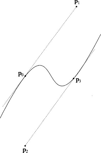
It's interesting to note that the top and bottom rows are points on the curve itself. p₀ is the point at the homogeneous parameter value [0,1] (or at T = 0 in the nonhomogeneous formulation), and p₃ is the point at the homogeneous parameter value [1,0] (or at $T=\infty$ in the nonhomogeneous formulation). Furthermore, the line through p₀ and p₁ is tangent to the curve at p₀. And the line through p₂ and p₃ is tangent to the curve at p₃ (see Figure 15.1). Anyway, we can now rewrite the definition of the elements of the D vector from Equation (15.6) as

$\begin{array}{ccc}{D}_3& =& \text{?}\text{?}\text{?}{p}_2\cdot p_1\times p_0\\ D_2& =& -p_3\cdot p_1\times p_0\\ D_1& =& \text{?}\text{?}\text{?}{p}_3\cdot p_2\times p_0\\ D_0& =& -p_3\cdot p_2\times p_1\end{array}$

And the geometric transformation matrix we were using as our canonical transformation is simply

$M={\left[\begin{array}{l}\cdots p_3\cdots \\ \cdots p_2\cdots \\ \cdots p_1\cdots \end{array}\right]}^{-1}$

We can evaluate the matrix inverse from the cross products of the various row vectors. Each cross product gives a column vector, and the inverse is

${\left[\begin{array}{l}\cdots p_3\cdots \\ \cdots p_2\cdots \\ \cdots p_1\cdots \end{array}\right]}^{-1}=\frac{-1}{D_0}\text{?}\left[\begin{array}{ccc}⋮& ⋮& ⋮\\ p_2\times p_1& p_1\times p_3& p_3\times p_2\\ ⋮& ⋮& ⋮\end{array}\right]$

As long as this matrix is nonsingular (that is, the determinant, D₀, is nonzero), we can see that our canonical transformation will generate

$\begin{array}{l}\text{?}\text{?}\text{?}\text{?}\left[\begin{array}{l}\cdots p_3\cdots \\ \cdots p_2\cdots \\ \cdots p_1\cdots \\ \cdots p_0\cdots \end{array}\right]\text{?}{\left[\begin{array}{l}\cdots p_3\cdots \\ \cdots p_2\cdots \\ \cdots p_1\cdots \end{array}\right]}^{-1}\\ =\left[\begin{array}{l}\cdots p_3\cdots \\ \cdots p_2\cdots \\ \cdots p_1\cdots \\ \cdots p_0\cdots \end{array}\right]\frac{-1}{D_0}\left[\begin{array}{ccc}⋮& ⋮& ⋮\\ p_2\times p_1& p_1\times p_3& p_3\times p_2\\ ⋮& ⋮& ⋮\end{array}\right]\\ =\left[\begin{array}{ccc}1& 0& 0\\ 0& 1& 0\\ 0& 0& 1\\ -\frac{D_3}{D_0}& -\frac{D_2}{D_0}& -\frac{D_1}{D_0}\end{array}\right]\end{array}$

This, then, gives the meaning of the bottom row of the candidate canonical matrix. If, however, the original curve gave us a value of D₀ = 0, this is not a good choice for a canonical transformation. All is not lost, however. We can pick a transformation matrix as the inverse of any of the other subsets of three of the four rows and get the following possibilities for canonical coefficient matrices:

$\begin{array}{ccc}\left[\begin{array}{l}\cdots p_3\cdots \hfill \\ \cdots p_2\cdots \hfill \\ \cdots p_1\cdots \hfill \\ \cdots p_0\cdots \hfill \end{array}\right]\text{?}{\left[\begin{array}{l}\cdots p_3\cdots \hfill \\ \cdots p_2\cdots \hfill \\ \cdots p_0\cdots \hfill \end{array}\right]}^{-1}& =& \left[\begin{array}{ccc}1& 0& 0\\ 0& 1& 0\\ -\frac{D_3}{D_1}& -\frac{D_2}{D_1}& -\frac{D_0}{D_1}\\ 0& 0& 1\end{array}\right]\\ \left[\begin{array}{l}\cdots p_3\cdots \hfill \\ \cdots p_2\cdots \hfill \\ \cdots p_1\cdots \hfill \\ \cdots p_0\cdots \hfill \end{array}\right]\text{?}{\left[\begin{array}{l}\cdots p_2\cdots \hfill \\ \cdots p_1\cdots \hfill \\ \cdots p_0\cdots \hfill \end{array}\right]}^{-1}& =& \left[\begin{array}{ccc}1& 0& 0\\ -\frac{D_3}{D_2}& -\frac{D_1}{D_2}& -\frac{D_0}{D_2}\\ 0& 1& 0\\ 0& 0& 1\end{array}\right]\\ \left[\begin{array}{l}\cdots p_3\cdots \hfill \\ \cdots p_2\cdots \hfill \\ \cdots p_1\cdots \hfill \\ \cdots p_0\cdots \hfill \end{array}\right]\text{?}{\left[\begin{array}{l}\cdots p_2\cdots \hfill \\ \cdots p_1\cdots \hfill \\ \cdots p_0\cdots \hfill \end{array}\right]}^{-1}& =& \left[\begin{array}{ccc}-\frac{D_2}{D_3}& -\frac{D_1}{D_3}& -\frac{D_0}{D_3}\\ 1& 0& 0\\ 0& 1& 0\\ 0& 0& 1\end{array}\right]\end{array}$

Which of these is best to choose will depend on what values we have for the D_i's.

We have therefore been able to recast the question “How many different rational parametric cubic curves are there?” as “How many different homogeneous cubic polynomials are there?” We've gone from needing to understand the 12 numbers in the coefficient matrix to needing to understand the 4 coefficients in a homogeneous cubic polynomial.

How Does the Game Affect D?

The D vector determines where the inflection points are. The reason that inflection points are interesting is that the number of them will not change due to perspective transformations or due to reparametrization. How does this fact show up in the algebra of transformation that we just defined?

Winning the Game

The next order of business is to immerse ourselves in what types of homogeneous cubic polynomials exist under reparametrization. Our goal will be to pick a reparametrization matrix that makes the new values ${\widehat{D}}_i$ as simple as possible. We'll tackle that in the next millennium. (This was written just before New Year's Day 2000…. Oh, I really crack myself up.)