At this point, we know we need something else to read the data that was collected, transformed, and cataloged by Glue. You can see tables and schemas on Glue but you cannot see the content of the files, that is, the actual data. For that, we need to use Athena:

1. Go to the Console and open up the Athena console. If it's the first time you are doing this, the Get Started page will show up. Hit Get started and have a look at the interface:

The query editor is where the action happens: you can write SQL queries to interact with files directly. This means you don't have to set up expensive instances and relational databases before you can run some simple queries and aggregations on your data. Athena uses Presto to give you ANSI SQL functionality and supports several file formats.

On the left, you will see the database, which is exactly the list of databases you have on the Glue data catalog. Glue and Athena are strongly coupled and share the catalog. When you add databases and tables to Glue, they are also made available straight away in Athena.

2. With the weather database selected in the Athena console, you can see the two tables we created: raw for the raw data and weather_full for the transformed data.

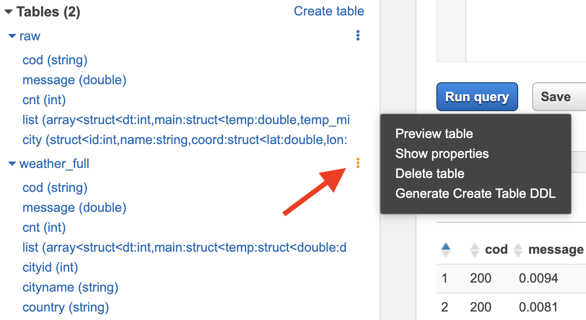
3. Expand the 2 tables to see their structure by clicking on the small arrow next to their names:

Our raw table has fewer columns because it has nested structures. Our weather_full table holds the flattened out structure that we created during our transformation process. Notice we still have an array (list) in our transformed data; we will play with that soon.

4. Click on the three stacked dots next to the weather_full table name and select Preview table from the menu:

A new query was created for you, limiting the results to 10 records:

SELECT * FROM "weather"."weather_full" limit 10;

Also, Athena gives you the amount of time the query took to run and the amount of scanned data. The reason for this is because Athena pricing is based on the amount of data your queries scan. When stored, Parquet files are smaller in size than JSON files for the same amount of data. Query efficiency for both cost and performance are the main reasons why we converted the JSON files into Parquet files for consumption. It would work if the transformed files were in JSON format as well, but for larger volumes of data, the performance would not be ideal and the amount of scanned data would be higher, meaning our overall cost would be higher as well.

Athena will scan data on S3 based on partitions. Normally, what goes into the WHERE clause in a SQL query tends to be a good candidate for a partitioning strategy. Certainly, every dataset may have different partitioning requirements that will be driven by business requirements but, for example, if most of the queries that are executed on an S3 dataset have a date filter, it is likely that the partitioning strategy will suggest data on S3 to be organized as something like the following:

bucket-name/2019/01/01/part-00960-b815f0d5-71d2-460d-ab63-75865dc9e1a4-c000.snappy.parquet
bucket-name/2019/01/01/part-00961-b815f0d5-71d2-460d-ab63-75865dc9e1a4-c000.snappy.parquet
...
bucket-name/2019/01/02/part-00958-b815f0d5-71d2-460d-ab63-75865dc9e1a4-c000.snappy.parquet
bucket-name/2019/01/02/part-00958-b815f0d5-71d2-460d-ab63-75865dc9e1a4-c000.snappy.parquet
...

By using that type of partitioning strategy, -bucket-name/YYYY/MM/DD/[data-files], when a business analyst runs a query that only retrieves data from the 1 Jan, 2019 (that is, WHERE date = '2019-01-01'), Athena will only scan data on the bucket-name/2019/01/01/ path instead of scanning the entire bucket, optimizing the query's performance and running costs.

The following query shows how you can access the data inside an array (the list column in our dataset) in a catalog table. You can take care of this in your transformation script and load a completely flat and denormalized dataset to be used on your queries, or you can access data within arrays by using the UNNEST operator, as per the following example:

SELECT
  full_list.dt_txt as ReadingTimeStamp,
  city.name as CityName,
  full_list.main.temp.double as Temperature,
  ...
  full_list.main.temp_kf.double as TemperatureKF,
  full_weather.main as WeatherMain,
  full_weather.description as WeatherDescription,
  full_list.wind.speed.double as WindSpeed,
  full_list.wind.deg.double as WindDeg
FROM
  "weather"."weather_full"
CROSS JOIN
  UNNEST(list) as t(full_list), UNNEST(full_list.weather) as s(full_weather)
LIMIT 10;

That concludes our  introduction to Athena. Now, you can run and experiment with SQL queries in the console.

Have a go at ingesting some other open datasets and using different transformation strategies. As a stretch goal, have a look at Amazon QuickSight for ways to turn your data and queries into visualizations.