
Most of the time, when working with contours, subjects will have the most diverse shapes, including convex ones. A convex shape is one where there are two points within this shape whose connecting line goes outside the perimeter of the shape itself.
The first facility that OpenCV offers to calculate the approximate bounding polygon of a shape is cv2.approxPolyDP. This function takes three parameters:
- A contour
- An epsilon value representing the maximum discrepancy between the original contour and the approximated polygon (the lower the value, the closer the approximated value will be to the original contour)
- A Boolean flag signifying that the polygon is closed
The epsilon value is of vital importance to obtain a useful contour, so let's understand what it represents. An epsilon is the maximum difference between the approximated polygon's perimeter and the original contour's perimeter. The lower this difference is, the more the approximated polygon will be similar to the original contour.
You may ask yourself why we need an approximate polygon when we have a contour that is already a precise representation. The answer to this is that a polygon is a set of straight lines, and the importance of being able to define polygons in a region for further manipulation and processing is paramount in many computer vision tasks.
Now that we know what an epsilon is, we need to obtain contour perimeter information as a reference value. This is obtained with the cv2.arcLength function of OpenCV:
epsilon = 0.01 * cv2.arcLength(cnt, True)
approx = cv2.approxPolyDP(cnt, epsilon, True)
Effectively, we're instructing OpenCV to calculate an approximated polygon whose perimeter can only differ from the original contour in an epsilon ratio.
OpenCV also offers a cv2.convexHull function to obtain processed contour information for convex shapes and this is a straightforward one-line expression:
hull = cv2.convexHull(cnt)
Let's combine the original contour, approximated polygon contour, and the convex hull in one image to observe the difference between them. To simplify things, I've applied the contours to a black image so that the original subject is not visible but its contours are:
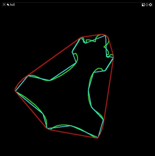
As you can see, the convex hull surrounds the entire subject, the approximated polygon is the innermost polygon shape, and in between the two is the original contour, mainly composed of arcs.