What is a feature exactly? Why is a particular area of an image classifiable as a feature, while others are not? Broadly speaking, a feature is an area of interest in the image that is unique or easily recognizable. As you can imagine, corners and high-density areas are good features, while patterns that repeat themselves a lot or low-density areas (such as a blue sky) are not. Edges are good features as they tend to divide two regions of an image. A blob (an area of an image that greatly differs from its surrounding areas) is also an interesting feature.

Most feature detection algorithms revolve around the identification of corners, edges, and blobs, with some also focusing on the concept of a ridge, which you can conceptualize as the symmetry axis of an elongated object (think, for example, about identifying a road in an image).

Some algorithms are better at identifying and extracting features of a certain type, so it's important to know what your input image is so that you can utilize the best tool in your OpenCV belt.

Detecting features – corners

Let's start by identifying corners by utilizing CornerHarris, and let's do this with an example. If you continue studying OpenCV beyond this book, you'll find that—for many a reason—chessboards are a common subject of analysis in computer vision, partly because a chequered pattern is suited to many types of feature detections, and maybe because chess is pretty popular among geeks.

Here's our sample image:

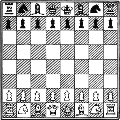
OpenCV has a very handy utility function called cornerHarris, which detects corners in an image. The code to illustrate this is incredibly simple:

import cv2
import numpy as np

img = cv2.imread('images/chess_board.png')
gray = cv2.cvtColor(img, cv2.COLOR_BGR2GRAY)
gray = np.float32(gray)
dst = cv2.cornerHarris(gray, 2, 23, 0.04)
img[dst>0.01 * dst.max()] = [0, 0, 255] 
while (True):
  cv2.imshow('corners', img)
  if cv2.waitKey(1000 / 12) & 0xff == ord("q"):
    break
cv2.destroyAllWindows()

Let's analyze the code: after the usual imports, we load the chessboard image and turn it to grayscale so that cornerHarris can compute it. Then, we call the cornerHarris function:

dst = cv2.cornerHarris(gray, 2, 23, 0.04)

The most important parameter here is the third one, which defines the aperture of the Sobel operator. The Sobel operator performs the change detection in the rows and columns of an image to detect edges, and it does this using a kernel. The OpenCV cornerHarris function uses a Sobel operator whose aperture is defined by this parameter. In plain english, it defines how sensitive corner detection is. It must be between 3 and 31 and be an odd value. At value 3, all those diagonal lines in the black squares of the chessboard will register as corners when they touch the border of the square. At 23, only the corners of each square will be detected as corners.

Consider the following line:

img[dst>0.01 * dst.max()] = [0, 0, 255] 

Here, in places where a red mark in the corners is detected, tweaking the second parameter in cornerHarris will change this, that is, the smaller the value, the smaller the marks indicating corners.

Here's the final result:

Great, we have corner points marked, and the result is meaningful at first glance; all the corners are marked in red.

The preceding technique, which uses cornerHarris, is great to detect corners and has a distinct advantage because corners are corners; they are detected even if the image is rotated.

However, if we reduce (or increase) the size of an image, some parts of the image may lose or even gain a corner quality.

For example, look at the following corner detections of the F1 Italian Grand Prix track:

Here's a smaller version of the same screenshot:

You will notice how corners are a lot more condensed; however, we didn't only gain corners, we also lost some! In particular, look at the Variante Ascari chicane that squiggles at the end of the NW/SE straight part of the track. In the larger version of the image, both the entrance and the apex of the double bend were detected as corners. In the smaller image, the apex is not detected as such. The more we reduce the image, the more likely it is that we're going to lose the entrance to that chicane too.

This loss of features raises an issue; we need an algorithm that will work regardless of the scale of the image. Enter SIFT: while Scale-Invariant Feature Transform may sound a bit mysterious, now that we know what problem we're trying to resolve, it actually makes sense. We need a function (a transform) that will detect features (a feature transform) and will not output different results depending on the scale of the image (a scale-invariant feature transform). Note that SIFT does not detect keypoints (which is done with Difference of Gaussians), but it describes the region surrounding them by means of a feature vector.

A quick introduction to Difference of Gaussians (DoG) is in order; we have already talked about low pass filters and blurring operations, specifically with the cv2.GaussianBlur() function. DoG is the result of different Gaussian filters applied to the same image. In Chapter 3, Processing Images with OpenCV 3, we applied this technique to compute a very efficient edge detection, and the idea is the same. The final result of a DoG operation contains areas of interest (keypoints), which are then going to be described through SIFT.

Let's see how SIFT behaves in an image full of corners and features:

Now, the beautiful panorama of Varese (Lombardy, Italy) also gains a computer vision meaning. Here's the code used to obtain this processed image:

import cv2
import sys
import numpy as np

imgpath = sys.argv[1]
img = cv2.imread(imgpath)

gray = cv2.cvtColor(img, cv2.COLOR_BGR2GRAY)

sift = cv2.xfeatures2d.SIFT_create()
keypoints, descriptor = sift.detectAndCompute(gray,None)

img = cv2.drawKeypoints(image=img, outImage=img, keypoints = keypoints, flags = cv2.DRAW_MATCHES_FLAGS_DRAW_RICH_KEYPOINT, color = (51, 163, 236))

cv2.imshow('sift_keypoints', img)
while (True):
  if cv2.waitKey(1000 / 12) & 0xff == ord("q"):
    break
cv2.destroyAllWindows()

After the usual imports, we load the image that we want to process. To make this script generic, we will take the image path as a command-line argument using the sys module of Python:

imgpath = sys.argv[1]
img = cv2.imread(imgpath)

gray = cv2.cvtColor(img, cv2.COLOR_BGR2GRAY)

We then turn the image into grayscale. At this stage, you may have gathered that most processing algorithms in Python need a grayscale feed in order to work.

The next step is to create a SIFT object and compute the grayscale image:

sift = cv2.xfeatures2d.SIFT_create()
keypoints, descriptor = sift.detectAndCompute(gray,None)

This is an interesting and important process; the SIFT object uses DoG to detect keypoints and computes a feature vector for the surrounding regions of each keypoint. As the name of the method clearly gives away, there are two main operations performed: detection and computation. The return value of the operation is a tuple containing keypoint information (keypoints) and the descriptor.

Finally, we process this image by drawing the keypoints on it and displaying it with the usual imshow function.

Note that in the drawKeypoints function, we pass a flag that has a value of 4. This is actually the cv2 module property:

cv2.DRAW_MATCHES_FLAGS_DRAW_RICH_KEYPOINT

This code enables the drawing of circles and orientation of each keypoint.

pt
size
angle
response
octave 
class_id

Computer vision is a relatively recent branch of computer science and many algorithms and techniques are of recent invention. SIFT is in fact only 16 years old, having been published by David Lowe in 1999.

SURF is a feature detection algorithm published in 2006 by Herbert Bay, which is several times faster than SIFT, and it is partially inspired by it.

It is not particularly relevant to this book to understand how SURF works under the hood, as much as we can use it in our applications and make the best of it. What is important to understand is that SURF is an OpenCV class that operates keypoint detection with the Fast Hessian algorithm and extraction with SURF, much like the SIFT class in OpenCV operating keypoint detection with DoG and extraction with SIFT.

Also, the good news is that as a feature detection algorithm, the API of SURF does not differ from SIFT. Therefore, we can simply edit the previous script to dynamically choose a feature detection algorithm instead of rewriting the entire program.

As we only support two algorithms for now, there is no need to find a particularly elegant solution to the evaluation of the algorithm to be used and we'll use the simple if blocks, as shown in the following code:

import cv2
import sys
import numpy as np

imgpath = sys.argv[1]
img = cv2.imread(imgpath)
alg = sys.argv[2]

def fd(algorithm):
  if algorithm == "SIFT":
    return cv2.xfeatures2d.SIFT_create()
  if algorithm == "SURF":
    return cv2.xfeatures2d.SURF_create(float(sys.argv[3]) if len(sys.argv) == 4 else 4000)

gray = cv2.cvtColor(img, cv2.COLOR_BGR2GRAY)

fd_alg = fd(alg)
keypoints, descriptor = fd_alg.detectAndCompute(gray,None)

img = cv2.drawKeypoints(image=img, outImage=img, keypoints = keypoints, flags = 4, color = (51, 163, 236))

cv2.imshow('keypoints', img)
while (True):
  if cv2.waitKey(1000 / 12) & 0xff == ord("q"):
    break
cv2.destroyAllWindows()

Here's the result using SURF with a threshold:

This image has been obtained by processing it with a SURF algorithm using a Hessian threshold of 8000. To be precise, I ran the following command:

> python feat_det.py images/varese.jpg SURF 8000

The higher the threshold, the less features identified, so play around with the values until you reach an optimal detection. In the preceding case, you can clearly see how individual buildings are detected as features.

In a process similar to the one we adopted in Chapter 4, Depth Estimation and Segmentation, when we were calculating disparity maps, try—as an exercise—to create a trackbar to feed the value of the Hessian threshold to the SURF instance, and see the number of features increase and decrease in an inversely proportional fashion.

Now, let's examine corner detection with FAST, the BRIEF keypoint descriptor, and ORB (which uses the two) and put feature detection to good use.

If SIFT is young, and SURF younger, ORB is in its infancy. ORB was first published in 2011 as a fast alternative to SIFT and SURF.

The algorithm was published in the paper, ORB: an efficient alternative to SIFT or SURF, and is available in the PDF format at http://www.vision.cs.chubu.ac.jp/CV-R/pdf/Rublee_iccv2011.pdf.

ORB mixes techniques used in the FAST keypoint detection and the BRIEF descriptor, so it is definitely worth taking a quick look at FAST and BRIEF first. We will then talk about Brute-Force matching—one of the algorithms used for feature matching—and show an example of feature matching.

FAST

The Features from Accelerated Segment Test (FAST) algorithm works in a clever way; it draws a circle around including 16 pixels. It then marks each pixel brighter or darker than a particular threshold compared to the center of the circle. A corner is defined by identifying a number of contiguous pixels marked as brighter or darker.

FAST implements a high-speed test, which attempts at quickly skipping the whole 16-pixel test. To understand how this test works, let's take a look at this screenshot:

As you can see, three out of four of the test pixels (pixels number 1, 9, 5, and 13) must be within (or beyond) the threshold (and, therefore, marked as brighter or darker) and one must be in the opposite side of the threshold. If all four are marked as brighter or darker, or two are and two are not, the pixel is not a candidate corner.

FAST is an incredibly clever algorithm, but not devoid of weaknesses, and to compensate these weaknesses, developers analyzing images can implement a machine learning approach, feeding a set of images (relevant to your application) to the algorithm so that corner detection is optimized.

Despite this, FAST depends on a threshold, so the developer's input is always necessary (unlike SIFT).

Now that we have a general idea of what FAST and BRIEF are, we can understand why the team behind ORB (at the time composed by Ethan Rublee, Vincent Rabaud, Kurt Konolige, and Gary R. Bradski) chose these two algorithms as a foundation for ORB.

In their paper, the authors aim at achieving the following results:

Aside from very technical jargon, the main points are quite clear; ORB aims at optimizing and speeding up operations, including the very important step of utilizing BRIEF in a rotation-aware fashion so that matching is improved even in situations where a training image has a very different rotation to the query image.

At this stage, though, I bet you have had enough of the theory and want to sink your teeth in some feature matching, so let's go look at some code.

As an avid listener of music, the first example that comes to my mind is to get the logo of a band and match it to one of the band's albums:

import numpy as np
import cv2
from matplotlib import pyplot as plt

img1 = cv2.imread('images/manowar_logo.png',cv2.IMREAD_GRAYSCALE)
img2 = cv2.imread('images/manowar_single.jpg', cv2.IMREAD_GRAYSCALE)

orb = cv2.ORB_create()
kp1, des1 = orb.detectAndCompute(img1,None)
kp2, des2 = orb.detectAndCompute(img2,None)
bf = cv2.BFMatcher(cv2.NORM_HAMMING, crossCheck=True)
matches = bf.match(des1,des2)
matches = sorted(matches, key = lambda x:x.distance)
img3 = cv2.drawMatches(img1,kp1,img2,kp2, matches[:40], img2,flags=2)
plt.imshow(img3),plt.show()

Let's now examine this code step by step.

After the usual imports, we load two images (the query image and the training image).

Note that you have probably seen the loading of images with a second parameter with the value of 0 being passed. This is because cv2.imread takes a second parameter that can be one of the following flags:

    IMREAD_ANYCOLOR = 4
    IMREAD_ANYDEPTH = 2
    IMREAD_COLOR = 1
    IMREAD_GRAYSCALE = 0
    IMREAD_LOAD_GDAL = 8
    IMREAD_UNCHANGED = -1

As you can see, cv2.IMREAD_GRAYSCALE is equal to 0, so you can pass the flag itself or its value; they are the same thing.

This is the image we've loaded:

This is another image that we've loaded:

Now, we proceed to creating the ORB feature detector and descriptor:

orb = cv2.ORB_create()
kp1, des1 = orb.detectAndCompute(img1,None)
kp2, des2 = orb.detectAndCompute(img2,None)

In a similar fashion to what we did with SIFT and SURF, we detect and compute the keypoints and descriptors for both images.

The theory at this point is pretty simple; iterate through the descriptors and determine whether they are a match or not, and then calculate the quality of this match (distance) and sort the matches so that we can display the top n matches with a degree of confidence that they are, in fact, matching features on both images.

BFMatcher, as described in Brute-Force matching, does this for us:

bf = cv2.BFMatcher(cv2.NORM_HAMMING, crossCheck=True)
matches = bf.match(des1,des2)
matches = sorted(matches, key = lambda x:x.distance)

At this stage, we already have all the information we need, but as computer vision enthusiasts, we place quite a bit of importance on visually representing data, so let's draw these matches in a matplotlib chart:

img3 = cv2.drawMatches(img1,kp1,img2,kp2, matches[:40], img2,flags=2)
plt.imshow(img3),plt.show()

The result is as follows:

There are a number of algorithms that can be used to detect matches so that we can draw them. One of them is K-Nearest Neighbors (KNN). Using different algorithms for different tasks can be really beneficial, because each algorithm has strengths and weaknesses. Some may be more accurate than others, some may be faster or less computationally expensive, so it's up to you to decide which one to use, depending on the task at hand.

For example, if you have hardware constraints, you may choose an algorithm that is less costly. If you're developing a real-time application, you may choose the fastest algorithm, regardless of how heavy it is on the processor or memory usage.

Among all the machine learning algorithms, KNN is probably the simplest, and while the theory behind it is interesting, it is well out of the scope of this book. Instead, we will simply show you how to use KNN in your application, which is not very different from the preceding example.

Crucially, the two points where the script differs to switch to KNN are in the way we calculate matches with the Brute-Force matcher, and the way we draw these matches. The preceding example, which has been edited to use KNN, looks like this:

import numpy as np
import cv2
from matplotlib import pyplot as plt

img1 = cv2.imread('images/manowar_logo.png',0)
img2 = cv2.imread('images/manowar_single.jpg',0)

orb = cv2.ORB_create()
kp1, des1 = orb.detectAndCompute(img1,None)
kp2, des2 = orb.detectAndCompute(img2,None)
bf = cv2.BFMatcher(cv2.NORM_HAMMING, crossCheck=True)
matches = bf.knnMatch(des1,des2, k=2)
img3 = cv2.drawMatchesKnn(img1,kp1,img2,kp2, matches, img2,flags=2)
plt.imshow(img3),plt.show()

The final result is somewhat similar to the previous one, so what is the difference between match and knnMatch? The difference is that match returns best matches, while KNN returns k matches, giving the developer the option to further manipulate the matches obtained with knnMatch.

For example, you could iterate through the matches and apply a ratio test so that you can filter out matches that do not satisfy a user-defined condition.

Finally, we are going to take a look at Fast Library for Approximate Nearest Neighbors (FLANN). The official Internet home of FLANN is at http://www.cs.ubc.ca/research/flann/.

Like ORB, FLANN has a more permissive license than SIFT or SURF, so you can freely use it in your project. Quoting the website of FLANN,

In other words, FLANN possesses an internal mechanism that attempts at employing the best algorithm to process a dataset depending on the data itself. FLANN has been proven to be 10 times times faster than other nearest neighbors search software.

FLANN is even available on GitHub at https://github.com/mariusmuja/flann. In my experience, I've found FLANN-based matching to be very accurate and fast as well as friendly to use.

Let's look at an example of FLANN-based feature matching:

import numpy as np
import cv2
from matplotlib import pyplot as plt

queryImage = cv2.imread('images/bathory_album.jpg',0)
trainingImage = cv2.imread('images/vinyls.jpg',0)

# create SIFT and detect/compute
sift = cv2.xfeatures2d.SIFT_create()
kp1, des1 = sift.detectAndCompute(queryImage,None)
kp2, des2 = sift.detectAndCompute(trainingImage,None)

# FLANN matcher parameters
FLANN_INDEX_KDTREE = 0
indexParams = dict(algorithm = FLANN_INDEX_KDTREE, trees = 5)
searchParams = dict(checks=50)   # or pass empty dictionary

flann = cv2.FlannBasedMatcher(indexParams,searchParams)

matches = flann.knnMatch(des1,des2,k=2)

# prepare an empty mask to draw good matches
matchesMask = [[0,0] for i in xrange(len(matches))]

# David G. Lowe's ratio test, populate the mask
for i,(m,n) in enumerate(matches):
    if m.distance < 0.7*n.distance:
        matchesMask[i]=[1,0]

drawParams = dict(matchColor = (0,255,0),
                   singlePointColor = (255,0,0),
                   matchesMask = matchesMask,
                   flags = 0)

resultImage = cv2.drawMatchesKnn(queryImage,kp1,trainingImage,kp2,matches,None,**drawParams)

plt.imshow(resultImage,), plt.show()

Some parts of the preceding script will be familiar to you at this stage (import of modules, image loading, and creation of a SIFT object).

We find that the FLANN matcher takes two parameters: an indexParams object and a searchParams object. These parameters, passed in a dictionary form in Python (and a struct in C++), determine the behavior of the index and search objects used internally by FLANN to compute the matches.

In this case, we could have chosen between LinearIndex, KTreeIndex, KMeansIndex, CompositeIndex, and AutotuneIndex, and we chose KTreeIndex. Why? This is because it's a simple enough index to configure (only requires the user to specify the number of kernel density trees to be processed; a good value is between 1 and 16) and clever enough (the kd-trees are processed in parallel). The searchParams dictionary only contains one field (checks) that specifies the number of times an index tree should be traversed. The higher the value, the longer it takes to compute the matching, but it will also be more accurate.

In reality, a lot depends on the input that you feed the program with. I've found that 5 kd-trees and 50 checks always yield a respectably accurate result, while only taking a short time to complete.

After the creation of the FLANN matcher and having created the matches array, matches are then filtered according to the test described by Lowe in his paper, Distinctive Image Features from Scale-Invariant Keypoints, available at https://www.cs.ubc.ca/~lowe/papers/ijcv04.pdf.

In its chapter, Application to object recognition, Lowe explains that not all matches are "good" ones, and that filtering according to an arbitrary threshold would not yield good results all the time. Instead, Dr. Lowe explains,

In the preceding example, discarding any value with a distance greater than 0.7 will result in just a few good matches being filtered out, while getting rid of around 90 percent of false matches.

Let's unveil the result of a practical example of FLANN. This is the query image that I've fed the script:

This is the training image:

Here, you may notice that the image contains the query image at position (5, 3) of this grid.

This is the FLANN processed result:

A perfect match!!

First of all, what is homography? Let's read a definition from the Internet:

If you—like me—are none the wiser from the preceding definition, you will probably find this explanation a bit clearer: homography is a condition in which two figures find each other when one is a perspective distortion of the other.

Unlike all the previous examples, let's first take a look at what we want to achieve so that we can fully understand what homography is. Then, we'll go through the code. Here's the final result:

As you can see from the screenshot, we took a subject on the left, correctly identified in the image on the right-hand side, drew matching lines between keypoints, and even drew a white border showing the perspective deformation of the seed subject in the right-hand side of the image:

import numpy as np
import cv2
from matplotlib import pyplot as plt

MIN_MATCH_COUNT = 10

img1 = cv2.imread('images/bb.jpg',0)
img2 = cv2.imread('images/color2_small.jpg',0)

sift = cv2.xfeatures2d.SIFT_create()
kp1, des1 = sift.detectAndCompute(img1,None)
kp2, des2 = sift.detectAndCompute(img2,None)

FLANN_INDEX_KDTREE = 0
index_params = dict(algorithm = FLANN_INDEX_KDTREE, trees = 5)
search_params = dict(checks = 50)

flann = cv2.FlannBasedMatcher(index_params, search_params)

matches = flann.knnMatch(des1,des2,k=2)

# store all the good matches as per Lowe's ratio test.
good = []
for m,n in matches:
    if m.distance < 0.7*n.distance:
        good.append(m)

if len(good)>MIN_MATCH_COUNT:
    src_pts = np.float32([ kp1[m.queryIdx].pt for m in good ]).reshape(-1,1,2)
    dst_pts = np.float32([ kp2[m.trainIdx].pt for m in good ]).reshape(-1,1,2)

    M, mask = cv2.findHomography(src_pts, dst_pts, cv2.RANSAC,5.0)
    matchesMask = mask.ravel().tolist()

    h,w = img1.shape
    pts = np.float32([ [0,0],[0,h-1],[w-1,h-1],[w-1,0] ]).reshape(-1,1,2)
    dst = cv2.perspectiveTransform(pts,M)

    img2 = cv2.polylines(img2,[np.int32(dst)],True,255,3, cv2.LINE_AA)

else:
    print "Not enough matches are found - %d/%d" % (len(good),MIN_MATCH_COUNT)
    matchesMask = None

draw_params = dict(matchColor = (0,255,0), # draw matches in green color
                   singlePointColor = None,
                   matchesMask = matchesMask, # draw only inliers
                   flags = 2)

img3 = cv2.drawMatches(img1,kp1,img2,kp2,good,None,**draw_params)

plt.imshow(img3, 'gray'),plt.show()

When compared to the previous FLANN-based matching example, the only difference (and this is where all the action happens) is in the if block.

Here's what happens in this code step by step: firstly, we make sure that we have at least a certain number of good matches (the minimum required to compute a homography is four), which we will arbitrarily set at 10 (in real life, you would probably use a higher value than this):

if len(good)>MIN_MATCH_COUNT:

Then, we find the keypoints in the original image and the training image:

src_pts = np.float32([ kp1[m.queryIdx].pt for m in good ]).reshape(-1,1,2)
dst_pts = np.float32([ kp2[m.trainIdx].pt for m in good ]).reshape(-1,1,2)

Now, we find the homography:

M, mask = cv2.findHomography(src_pts, dst_pts, cv2.RANSAC,5.0)
matchesMask = mask.ravel().tolist()

Note that we create matchesMask, which will be used in the final drawing of the matches so that only points lying within the homography will have matching lines drawn.

At this stage, we simply have to calculate the perspective distortion of the original object into the second picture so that we can draw the border:

h,w = img1.shape
pts = np.float32([ [0,0],[0,h-1],[w-1,h-1],[w-1,0] ]).reshape(-1,1,2)
dst = cv2.perspectiveTransform(pts,M)
img2 = cv2.polylines(img2,[np.int32(dst)],True,255,3, cv2.LINE_AA)

And we then proceed to draw as per all our previous examples.

Let's conclude this chapter with a real-life (or kind of) example. Imagine that you're working for the Gotham forensics department and you need to identify a tattoo. You have the original picture of the tattoo (imagine this coming from a CCTV footage) belonging to a criminal, but you don't know the identity of the person. However, you possess a database of tattoos, indexed with the name of the person to whom the tattoo belongs.

So, let's divide the task in two parts: save image descriptors to files first, and then, scan these for matches against the picture we are using as a query image.

# generate_descriptors.py
import cv2
import numpy as np
from os import walk
from os.path import join
import sys

def create_descriptors(folder):
  files = []
  for (dirpath, dirnames, filenames) in walk(folder):
    files.extend(filenames)
  for f in files:
    save_descriptor(folder, f, cv2.xfeatures2d.SIFT_create())

def save_descriptor(folder, image_path, feature_detector):
  img = cv2.imread(join(folder, image_path), 0)
  keypoints, descriptors = feature_detector.detectAndCompute(img, None)
  descriptor_file = image_path.replace("jpg", "npy")
  np.save(join(folder, descriptor_file), descriptors)

dir = sys.argv[1]

create_descriptors(dir)

> python generate_descriptors.py <folder containing images>

Scanning for matches

Now that we have descriptors saved to files, all we need to do is to repeat the homography process on all the descriptors and find a potential match to our query image.

This is the process we will put in place:

• Loading a query image and creating a descriptor for it (tattoo_seed.jpg)
• Scanning the folder with descriptors
• For each descriptor, computing a FLANN-based match
• If the number of matches is beyond an arbitrary threshold, including the file of potential culprits (remember we're investigating a crime)
• Of all the culprits, electing the one with the highest number of matches as the potential suspect

Let's inspect the code to achieve this:

from os.path import join
from os import walk
import numpy as np
import cv2
from sys import argv

# create an array of filenames
folder = argv[1]
query = cv2.imread(join(folder, "tattoo_seed.jpg"), 0)

# create files, images, descriptors globals
files = []
images = []
descriptors = []
for (dirpath, dirnames, filenames) in walk(folder):
  files.extend(filenames)
  for f in files:
    if f.endswith("npy") and f != "tattoo_seed.npy":
      descriptors.append(f)
  print descriptors

# create the sift detector
sift = cv2.xfeatures2d.SIFT_create()
query_kp, query_ds = sift.detectAndCompute(query, None)

# create FLANN matcher
FLANN_INDEX_KDTREE = 0
index_params = dict(algorithm = FLANN_INDEX_KDTREE, trees = 5)
search_params = dict(checks = 50)
flann = cv2.FlannBasedMatcher(index_params, search_params)

# minimum number of matches
MIN_MATCH_COUNT = 10

potential_culprits = {}

print ">> Initiating picture scan..."
for d in descriptors:
  print "--------- analyzing %s for matches ------------" % d
  matches = flann.knnMatch(query_ds, np.load(join(folder, d)), k =2)
  good = []
  for m,n in matches:
      if m.distance < 0.7*n.distance:
          good.append(m)
  if len(good) > MIN_MATCH_COUNT:
    print "%s is a match! (%d)" % (d, len(good))
  else:
    print "%s is not a match" % d
  potential_culprits[d] = len(good)

max_matches = None
potential_suspect = None
for culprit, matches in potential_culprits.iteritems():
  if max_matches == None or matches > max_matches:
    max_matches = matches
    potential_suspect = culprit

print "potential suspect is %s" % potential_suspect.replace("npy", "").upper()

I saved this script as scan_for_matches.py. The only element of novelty in this script is the use of numpy.load(filename), which loads an npy file into an np array.

Running the script produces the following output:

>> Initiating picture scan...
--------- analyzing posion-ivy.npy for matches ------------
posion-ivy.npy is not a match
--------- analyzing bane.npy for matches ------------
bane.npy is not a match
--------- analyzing two-face.npy for matches ------------
two-face.npy is not a match
--------- analyzing riddler.npy for matches ------------
riddler.npy is not a match
--------- analyzing penguin.npy for matches ------------
penguin.npy is not a match
--------- analyzing dr-hurt.npy for matches ------------
dr-hurt.npy is a match! (298)
--------- analyzing hush.npy for matches ------------
hush.npy is a match! (301)
potential suspect is HUSH.

If we were to represent this graphically, this is what we would see: