Let's look at an example. We start with the picture of a beautiful statue of an angel.

We want to grab our angel and discard the background. To do this, we will create a relatively short script that will instantiate GrabCut, operate the separation, and then display the resulting image side by side to the original. We will do this using matplotlib, a very useful Python library, which makes displaying charts and images a trivial task:

import numpy as np
import cv2
from matplotlib import pyplot as plt

img = cv2.imread('images/statue_small.jpg')
mask = np.zeros(img.shape[:2],np.uint8)

bgdModel = np.zeros((1,65),np.float64)
fgdModel = np.zeros((1,65),np.float64)

rect = (100,50,421,378)
cv2.grabCut(img,mask,rect,bgdModel,fgdModel,5,cv2.GC_INIT_WITH_RECT)

mask2 = np.where((mask==2)|(mask==0),0,1).astype('uint8')
img = img*mask2[:,:,np.newaxis]

plt.subplot(121), plt.imshow(img)
plt.title("grabcut"), plt.xticks([]), plt.yticks([])
plt.subplot(122), plt.imshow(cv2.cvtColor(cv2.imread('images/statue_small.jpg'), cv2.COLOR_BGR2RGB))
plt.title("original"), plt.xticks([]), plt.yticks([])
plt.show()

This code is actually quite straightforward. Firstly, we load the image we want to process, and then we create a mask populated with zeros with the same shape as the image we've loaded:

import numpy as np
import cv2
from matplotlib import pyplot as plt

img = cv2.imread('images/statue_small.jpg')
mask = np.zeros(img.shape[:2],np.uint8)

We then create zero-filled foreground and background models:

bgdModel = np.zeros((1,65),np.float64)
fgdModel = np.zeros((1,65),np.float64)

We could have populated these models with data, but we're going to initialize the GrabCut algorithm with a rectangle identifying the subject we want to isolate. So, background and foreground models are going to be determined based on the areas left out of the initial rectangle. This rectangle is defined in the next line:

rect = (100,50,421,378)

Now to the interesting part! We run the GrabCut algorithm specifying the empty models and mask, and the fact that we're going to use a rectangle to initialize the operation:

cv2.grabCut(img,mask,rect,bgdModel,fgdModel,5,cv2.GC_INIT_WITH_RECT)

You'll also notice an integer after fgdModel, which is the number of iterations the algorithm is going to run on the image. You can increase these, but there is a point in which pixel classifications will converge, and effectively, you'll just be adding iterations without obtaining any more improvements.

After this, our mask will have changed to contain values between 0 and 3. The values, 0 and 2, will be converted into zeros, and 1-3 into ones, and stored into mask2, which we can then use to filter out all zero-value pixels (theoretically leaving all foreground pixels intact):

mask2 = np.where((mask==2)|(mask==0),0,1).astype('uint8')
img = img*mask2[:,:,np.newaxis]

The last part of the code displays the images side by side, and here's the result:

This is quite a satisfactory result. You'll notice that an area of background is left under the angel's arm. It is possible to apply touch strokes to apply more iterations; the technique is quite well illustrated in the grabcut.py file in samples/python2 of your OpenCV installation.

Finally, we take a quick look at the Watershed algorithm. The algorithm is called Watershed, because its conceptualization involves water. Imagine areas with low density (little to no change) in an image as valleys, and areas with high density (lots of change) as peaks. Start filling the valleys with water to the point where water from two different valleys is about to merge. To prevent the merging of water from different valleys, you build a barrier to keep them separated. The resulting barrier is the image segmentation.

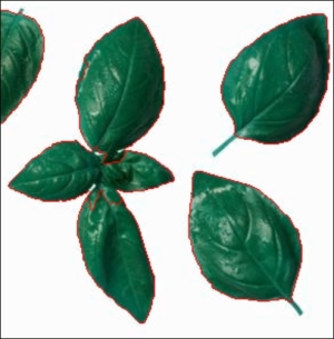
As an Italian, I love food, and one of the things I love the most is a good plate of pasta with a pesto sauce. So here's a picture of the most vital ingredient for a pesto, basil:

Now, we want to segment the image to separate the basil leaves from the white background.

Once more, we import numpy, cv2, and matplotlib, and then import our basil leaves' image:

import numpy as np
import cv2
from matplotlib import pyplot as plt
img = cv2.imread('images/basil.jpg')
gray = cv2.cvtColor(img,cv2.COLOR_BGR2GRAY)

After changing the color to grayscale, we run a threshold on the image. This operation helps dividing the image in two, blacks and whites:

ret, thresh = cv2.threshold(gray,0,255,cv2.THRESH_BINARY_INV+cv2.THRESH_OTSU)

Next up, we remove noise from the image by applying the morphologyEx transformation, an operation that consists of dilating and then eroding an image to extract features:

kernel = np.ones((3,3),np.uint8)
opening = cv2.morphologyEx(thresh,cv2.MORPH_OPEN,kernel, iterations = 2)

By dilating the result of the morphology transformation, we can obtain areas of the image that are most certainly background:

sure_bg = cv2.dilate(opening,kernel,iterations=3)

Conversely, we can obtain sure foreground areas by applying distanceTransform. In practical terms, of all the areas most likely to be foreground, the farther away from the "border" with the background a point is, the higher the chance it is foreground. Once we've obtained the distanceTransform representation of the image, we apply a threshold to determine with a highly mathematical probability whether the areas are foreground:

dist_transform = cv2.distanceTransform(opening,cv2.DIST_L2,5)
ret, sure_fg = cv2.threshold(dist_transform,0.7*dist_transform.max(),255,0)

At this stage, we have some sure foregrounds and backgrounds. Now, what about the areas in between? First of all, we need to determine these regions, which can be done by subtracting the sure foreground from the background:

sure_fg = np.uint8(sure_fg)
unknown = cv2.subtract(sure_bg,sure_fg)

Now that we have these areas, we can build our famous "barriers" to stop the water from merging. This is done with the connectedComponents function. We took a glimpse at the graph theory when we analyzed the GrabCut algorithm, and conceptualized an image as a set of nodes that are connected by edges. Given the sure foreground areas, some of these nodes will be connected together, but some won't. This means that they belong to different water valleys, and there should be a barrier between them:

ret, markers = cv2.connectedComponents(sure_fg)

Now we add 1 to the background areas because we only want unknowns to stay at 0:

markers = markers+1
markers[unknown==255] = 0

Finally, we open the gates! Let the water fall and our barriers be drawn in red:

markers = cv2.watershed(img,markers)
img[markers == -1] = [255,0,0]
plt.imshow(img)
plt.show()

Now, let's show the result:

Needless to say, I am now hungry!