CHAPTER EIGHT
Additional Topics
8.1 HERMITIAN MATRICES AND THE SPECTRAL THEOREM
It is clear that the chief end of mathematical study must be to make the student think.
—JOHN WESLEY YOUNG (1880–1932)
Cogito Ergo Sum. I think, therefore I am.
—RENÉ DESCARTES (1596–1650)
Introduction
In Section 5.3 on coordinate systems, we saw instances of a linear transformation that could be put into a simple form—at the expense of changing the basis of the underlying space. Later, in Section 5.3, we saw how to find a basis so that a given linear transformation would be represented by a diagonal matrix. This turned out to be possible in some cases, but not in all. Here we take up this theme again, and shall find that for a symmetric real matrix or Hermitian complex matrix, the situation is favorable: The diagonalization is always possible, and the new basis is orthonormal. Further, the eigenvalues of matrices that are symmetric and Hermitian are necessarily real. It is easy to see why these theorems are regarded as pinnacles in the theory of linear algebra. The main results are two versions of the Spectral Theorems (Theorems 6–7).
Hermitian Matrices and Self-Adjoint Mappings
We proceed in as general a way as possible. Thus, we consider arbitrary inner-product spaces and linear maps rather than limiting ourselves to ![]() and matrices. Furthermore, it is better to consider inner-product spaces in which the scalars are allowed to be complex numbers. The first important example of this is the space
and matrices. Furthermore, it is better to consider inner-product spaces in which the scalars are allowed to be complex numbers. The first important example of this is the space ![]() , whose elements are vectors with n complex components. The standard inner product in
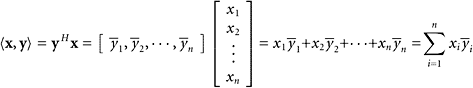
, whose elements are vectors with n complex components. The standard inner product in ![]() is
is
 |
|
If a vector y in ![]() is regarded as an n × 1 matrix, (i.e., a column vector), then yH is the corresponding row vector, with the conjugates of the components in place of the original components.
is regarded as an n × 1 matrix, (i.e., a column vector), then yH is the corresponding row vector, with the conjugates of the components in place of the original components.
DEFINITION
A matrix A is Hermitian1 if A = AH. Equivalently, the entries in A must obey this rule: aij = ![]() ji.
ji.
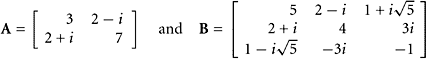
EXAMPLE 1
Show Hermitian matrices containing some imaginary numbers.
1 Charles Hermite (1822–1901) is remembered for many accomplishments in mathematics, one of the first being his establishing in 1873 that the number e is transcendental. (That means that e is not the root of any polynomial whose coefficients are integers.) Later, Hermite’s name was attached to an orthogonal system of polynomials that eventually played a crucial role in quantum mechanics. Hermite had a defect in his right foot and walked with some difficulty. After a year in the university, he was refused the right to continue his studies because of this disability! Although this unfair decision was reversed after pressure from some important people, Hermite decided he did not want to stay under the strict conditions imposed on him. Four years later, in recognition of his brilliant research, he was appointed to a faculty position at the same institution that had tried to prevent him from continuing his studies.
SOLUTION
 |
|
EXAMPLE 2
Illustrate some algebraic operations in ![]() .
.
SOLUTION Notice that
 |
|
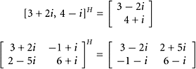
Moreover, for two given vectors
|
we find that
|
A real matrix is Hermitian if and only if it is symmetric. This fact is obvious from the definition of ‘‘Hermitian.’’ Thus, we have generalized the concept of symmetric to Hermitian. However, there is this twist that after taking the transpose, we also take the complex conjugates of all entries. In an inner-product space with complex vectors, we must remember that
|
and
|
A consequence is that for a square matrix A, we have
|
In this setting, we often use the notation AH to denote the conjugate transpose of a matrix A. It is obtained by taking the transpose of A and then replacing each entry by its complex conjugate. The order of these two steps can be reversed. In symbols: ![]() , or
, or ![]() . (If z = α + iβ, where α and β are real, then the conjugate of the complex number z is
. (If z = α + iβ, where α and β are real, then the conjugate of the complex number z is ![]() .) In matrix notation, we have
.) In matrix notation, we have
|
Then, we have
|
Notice that if we use the inner-product notation, it is inconsequential whether the vectors are regarded as rows or columns. For the matrix version of the inner product, however, a vector y must be treated as a column vector, and then yH is a row vector. The so-called outer product of two n-component vectors is also defined; it is
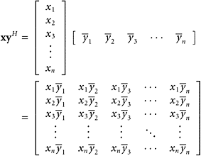 |
|
and is an n × n matrix of rank at most one.
Self-Adjoint Mapping
The concept of a matrix being Hermitian corresponds to the concept of a self-adjoint mapping in an inner-product space.
DEFINITION
A mapping f from an inner-product space into itself is self-adjoint if the equation
|
is true for all vectors x and y. In this definition, the scalar field for the inner-product space may be either ![]() or
or ![]() .
.
THEOREM 1
Every self-adjoint mapping is linear.
PROOF Let f be self-adjoint. For given vectors x and y, we have, for an arbitrary vector z
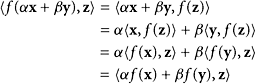 |
|
Since z is arbitrary, we conclude that f(αx + βy) = αf(x) + βf(y) and f is linear.
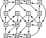
THEOREM 2
All eigenvalues of a self-adjoint operator are real.
PROOF Let L be a self-adjoint operator on some inner-product space, and suppose that
|
for some nonzero x. (At this stage in the proof, the eigenvalue λ is allowed to be complex.) We have
|
Cancelling the nonzero term ![]() leaves the equation
leaves the equation ![]() ; whence, λ must be real.
; whence, λ must be real.
THEOREM 3
Any two eigenvectors of a self-adjoint operator, if associated with different eigenvalues, are mutually orthogonal.
PROOF Let L be a self-adjoint transformation on an inner-product space. Suppose that
|
It may be assumed that x and y are nonzero vectors and that λ ≠ µ. By straightforward calculation, it is revealed that
|
(Notice that Theorem 2 allowed us to write ![]() .) Since λ ≠ µ, it must be that
.) Since λ ≠ µ, it must be that ![]() .
.
THEOREM 4
Consider ![]() with its standard inner product, and let A be an n × n matrix. Define a linear transformation L by writing L(x) = Ax, where x ∈
with its standard inner product, and let A be an n × n matrix. Define a linear transformation L by writing L(x) = Ax, where x ∈ ![]() . The operator L is self-adjoint if and only if A is Hermitian.
. The operator L is self-adjoint if and only if A is Hermitian.
PROOF We have the following equivalences, where, for brevity, we have omitted all the universal quantifiers ‘‘for all x’’ and ‘‘for all y.’’ The symbol ![]() means ‘‘if and only if .’’
means ‘‘if and only if .’’
|
COROLLARY 1
All eigenvalues of a Hermitian matrix are real.
PROOF If A is Hermitian and L(x) = Ax, then L is self-adjoint, by Theorem 4. The eigenvalues of A and L are the same and are real, by Theorem 2.
COROLLARY 2
All eigenvalues of a symmetric real matrix are real.
THEOREM 5
Let L be a linear transformation on a finite-dimensional vector space. If A is the matrix for L relative to a given basis, then the eigenvalues of L and A are the same.
PROOF Recall Theorem 4 in Section 5.3. According to it, if the basis in question is ![]() , then the matrix A plays this role:
, then the matrix A plays this role:
|
for every point x in the space. Now we have these equivalences:
|
EXAMPLE 3
Find the eigenvalues of the first matrix in Example 1.
SOLUTION Since ![]() and is Hermitian, its eigenvalues must be real. To calculate the eigenvalues, we find the roots of the characteristic polynomial:
and is Hermitian, its eigenvalues must be real. To calculate the eigenvalues, we find the roots of the characteristic polynomial:
 |
|
Hence, the eigenvalues are 2 and 8.
EXAMPLE 4
Find the eigenvectors for the matrix A in the preceding example. Are they mutually orthogonal?
SOLUTION Taking λ = 2, we find an eigenvector ![]() . Taking λ = 8, we find an eigenvector
. Taking λ = 8, we find an eigenvector ![]() . We have
. We have ![]() . Yes, they are!
. Yes, they are!
The Spectral Theorem
Now we present a version of the spectral theorem that is as brief as possible. The reader will see at once how it reveals the structure of any self-adjoint operator. Endearing properties of the eigenvalues and eigenspaces will result easily from the spectral theorem.
THEOREM 6 Spectral Theorem
Let L be a self-adjoint operator on an n-dimensional inner-product space, X. (The scalar field for X can be either ![]() or
or ![]() .) Then there exists an orthonormal basis {u1, u2, …, un} for X and a set of n real numbers λj such that
.) Then there exists an orthonormal basis {u1, u2, …, un} for X and a set of n real numbers λj such that
|
PROOF We begin by noticing that if the preceding displayed equation is true, then we can infer that
|
Thus, the vectors uj are eigenvectors of L, and the numbers λj are corre sponding eigenvalues of L. Select an eigenvalue, say λ1, together with an eigenvector u1, which we may assume to be a unit vector. By Theorem 2, λ1 is real. This is Step 1 in an n-step process.
Let us describe a typical step, say Step k, where k < n. Suppose that we have chosen eigenvalues λ1, λ2,…,λk (not necessarily distinct). Suppose also that we have an orthonormal set {u1, u2, …, uk}, where
|
Let V be the span of {u1, u2, …, uk}. We restrict the operator L to V![]() , and discover that V is invariant under L. This means that L(V
, and discover that V is invariant under L. This means that L(V![]() ) ⊆ V
) ⊆ V![]() . Indeed, if x ∈ V
. Indeed, if x ∈ V![]() , then, for j in the range 1 ≤ j ≤ k, we have
, then, for j in the range 1 ≤ j ≤ k, we have
|
This establishes that
|
The restricted operator is written L|V![]() . (It is the same as L, except for its having a smaller domain, namely V
. (It is the same as L, except for its having a smaller domain, namely V![]() .) It is also self-adjoint. Hence, we can find an eigen value λk+1 and an eigenvector uk+1 (taken to be of unit length) in V
.) It is also self-adjoint. Hence, we can find an eigen value λk+1 and an eigenvector uk+1 (taken to be of unit length) in V![]() . We know that uk+1 is orthogonal to {u1, u2, …, uk}. This process is repeated until we have found n eigenvalues and n eigenvectors. (The eigenvalues are not necessarily distinct. For a given eigenvalue, there may be several mutually orthogonal eigenvectors.) When the process stops, we have an orthonormal base for the space. Hence for each x, we have
. We know that uk+1 is orthogonal to {u1, u2, …, uk}. This process is repeated until we have found n eigenvalues and n eigenvectors. (The eigenvalues are not necessarily distinct. For a given eigenvalue, there may be several mutually orthogonal eigenvectors.) When the process stops, we have an orthonormal base for the space. Hence for each x, we have
|
whence we obtain
|
Unitary and Orthogonal Matrices
DEFINITION
A square matrix U is unitary if UH U = I. If U is real and UT U = I, the term orthogonal is used.
The matrix version of the Spectral Theorem is as follows. It uses the concept of a unitary matrix.
THEOREM 7 Spectral Theorem: Matrix Version
Let A be a Hermitian matrix. Then there exists a unitary matrix U such that
|
where D is a diagonal matrix having all the eigenvalues of A on its diagonal. The columns of U are unit eigenvectors of A.
PROOF Define an operator L on ![]() by the equation
by the equation
|
By Theorem 4, L is self-adjoint. Hence, by the Spectral Theorem, we have
|
We use the notation (uk)j to represent the jth component of the vector uk. Let U be the matrix whose columns are u1, u2, …, un. Then (uk)i = Uik. From the preceding equation, we then can write
|
Consequently, we have
|
Now let D be the diagonal matrix with the eigenvalues on its diagonal, Dνµ = λνδνµ. Then we can continue the preceding calculation of A as follows:
|
This equation means that A = UDUH.
EXAMPLE 5
Find the eigenvalues of the matrix ![]() and the unitary matrix U such the UHAU = D.
and the unitary matrix U such the UHAU = D.
SOLUTION Being Hermitian, A must have real eigenvalues. In the usual way, we find these to be 11 and 1. The corresponding eigenvectors are v =[3i, 1]T and w =[1, 3i]T. This pair is orthogonal:
|
We can normalize these two eigenvectors and put them as columns in a matrix, U. Thus, we have ![]() . The matrix U satisfies UUH = I and U−1 = UH.
. The matrix U satisfies UUH = I and U−1 = UH.
THEOREM 8
Let A be a real, symmetric matrix. Then there is an orthogonal matrix U such that
|
where D is a diagonal matrix having the eigenvalues of A on its diagonal. The columns of U are the corresponding eigenvectors of unit length.
PROOF This is the special case of Theorem 7 that arises when A is real.
Theorem 7 is often summarized by saying that a Hermitian matrix is unitarily similar to a diagonal matrix. Recall that similar means the relationship A = SBS−1 holds for two matrices, A and B. When we say unitarily similar, we mean that A = UBU−1, where U is a unitary matrix. Thus, we have UUH = I and the inverse of U is UH; that is, U−1 = UH.
DEFINITION
Two matrices A and B are unitarily similar to each other if there is a unitary matrix U such that A = UBUH.
Likewise, Theorem 8 is summarized by saying that a symmetric, real matrix is orthogonally similar to a diagonal matrix. In this case, U should be an orthogonal matrix: UUT = I. Theorems 6, 7, and 8 are often regarded as high points in the subject of linear algebra.
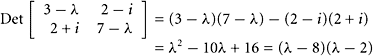
SOLUTION The characteristic polynomial is (3 − λ)2 + 16i2 = λ2 − 6λ − 7 and its roots (eigenvalues of A) are 7 and −1. Taking the eigenvalue 7, we find a corresponding eigenvector by solving the equation (A−7 I)x = 0. A convenient solution (not normalized) is [i, 1]T. The normalized eigenvector is then [c i, c]T, where ![]() . We treat the second eigenvalue, −1, in the same way and find the normalized eigenvector [c i, −c]T. These normalized eigenvectors go into a matrix U as columns, keeping the correct order. Thus, we obtain
. We treat the second eigenvalue, −1, in the same way and find the normalized eigenvector [c i, −c]T. These normalized eigenvectors go into a matrix U as columns, keeping the correct order. Thus, we obtain ![]() . To verify all the important conclusions, we calculate
. To verify all the important conclusions, we calculate
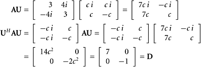 |
|
We can view this as a factorization of the matrix A:
|
Recall that this equation allows us to compute Ak efficiently:
|
The powers of the diagonal matrix D are ![]() .
.
The Cayley–Hamilton Theorem
We turn now to a remarkable theorem, named after Arthur Cayley2 and Sir William Rowan Hamilton3. One of the important mathematicians of the nineteenth century was Arthur Cayley. In an 1858 paper entitled A Memoir on the Theory of Matrices, he wrote the following passage: ‘‘I obtain the remarkable theorem that any matrix whatever satisfies an algebraic equation of its own order, the coefficient of the highest power being unity… and the last coefficient being in fact the determinant.’’ The formal statement of this result is Theorem 9.
2 Arthur Cayley (1821–1895) published three mathematical papers while still an undergraduate! He spent 14 years working as a lawyer so that he could retire and pursue mathematics. He published about 250 mathematical papers. If anybody should be credited as the creator of matrix theory, Cayley might be the best choice. He also was a learned man in other diffuse areas, such as law, literature, and architecture. He showed that our present-day definition of matrix multiplication is the correct one from the standpoint of linear operator theory (preserving the composition of two linear maps). He also studied quadratic forms and matrix inverses. Cayley’s accomplishments must be appreciated in the context of nineteenth-century mathematics. Many mathematicians shrank from participating in matrix theory, principally because the product of matrices is not commutative! In their eyes, that flaw in the theory discredited the entire subject.
3 William Rowan Hamilton (1805–1865) was a genius, able to read Latin, Greek, and Hebrew by the age of 5. At Trinity College, Dublin, he excelled in mathematics and physics, especially the subject of optics, to which he made substantial contributions. In mathematics, he is remembered chiefly as the inventor of quaternions, which are four-dimensional vectors with special noncommutative rules for multiplication.
THEOREM 9 Cayley–Hamilton Theorem
Every square matrix satisfies its own characteristic equation.
To understand this, recall first that the characteristic equation of a matrix A is
|
The lefthand side of this equation is a polynomial in the variable λ, and we have named it p. The zeros of the polynomial p are the eigenvalues of A. (Recall that one conceptually appealing algorithm for finding the eigenvalues of A is to compute the roots of the characteristic equation—that is, to solve for the zeros of p.)
In the characteristic polynomial, we are free to replace λ with any mathematical entity for which p(…) is meaningful. Thus, we can contemplate p(A), because the positive integer powers of A are well defined, and we can agree on using A0 = I. The Cayley–Hamilton Theorem asserts that
|
EXAMPLE 7
Let ![]()
Verify that A obeys the Cayley–Hamilton Theorem.
SOLUTION We find the characteristic polynomial of A:
|
Substituting A for λ produces
 |
|
In this same example, we could use the factored form of the characteristic polynomial, which is given by p(λ) = (λ + 1)(λ − 13). Substituting A for λ, we get
|
When A is assumed to be a diagonalizable matrix, a proof of the Cayley–Hamilton Theorem is not difficult! Here are the steps. Let
|
As we saw in Section 6.1,
|
for all k, and we have q(A) = Pq(D) P−1, for any polynomial q. If D = Diag(λ1, λ2, …,λn), then ![]() , and
, and
|
In particular, if q is the characteristic polynomial, then q(D) = 0, and q(A) = 0.
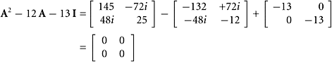
EXAMPLE 8
Let 
Find the coefficients in the equation A3 = c0I + c1A + c2A2.
SOLUTION Let the characteristic polynomial of A be p.Then
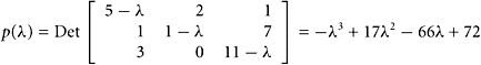 |
|
By the Cayley–Hamilton Theorem, p(A) = −A3 + 17A2 − 66A + 72I = 0, and the coefficients asked for are c0 = 72, c1 = −66, and c2 = 17.
EXAMPLE 9
Use the information in the preceding example to obtain A−1 in terms of the powers of A.
SOLUTION From Example 8, we have
|
Hence, we obtain
|
EXAMPLE 10
Use the Cayley–Hamilton Theorem to find the span of a set {I, A, A2, A3,…}, where A is an arbitrary n × n matrix.
SOLUTION The Cayley–Hamilton Theorem asserts that
|
if the coefficients cj are taken from the characteristic polynomial of A.It follows that An is in the span of {I, A, A2, …, An−1}. Multiply the preceding equation by A to see that An+1 is also in the same span. All the powers Ak for k ≥ n are in the span of {I, A, A2, …, An−1}:
|
The powers of an n × n matrix span a vector space of dimension at most n in the n2-dimensional space ![]() .
.
Quadratic Forms
A quadratic form is any homogeneous polynomial of degree two in any number of variables. In this situation, homogeneous means that all the terms are of degree two. For example, the expression 7x1x2 + 3x2x4 is homogeneous, but the expression x1 − 3x1x2 is not. The square of the distance between two points in an inner-product space is a quadratic form. Quadratic forms were introduced by Hermite, and 70 years later they turned out to be essential in the theory of quantum mechanics! The formal definition follows.
DEFINITION
A quadratic form is a function of this type: x ![]() xTAx. Here, A is an arbitrary n × n matrix and x is a vector variable in
xTAx. Here, A is an arbitrary n × n matrix and x is a vector variable in ![]() .
.
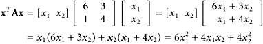
EXAMPLE 11
What is the explicit formula for the quadratic form that arises from the matrix ![]()
SOLUTION The quadratic form, according to the definition, is
 |
|
The resulting function is a polynomial of degree two in the variables x1 and x2, and each term is of degree two. We can think of it as a quadratic polynomial in two variables ax2 +2bxy + cy2.
This example illustrates the fact that a quadratic form induced by an n × n nonzero matrix is a polynomial of degree two in the n variables, x1,x2, …,xn.
If a quadratic form is presented as x ![]() xTBx, where B is a real matrix, then there is no loss of generality in requiring B to be symmetric. The next theorem restates and proves this.
xTBx, where B is a real matrix, then there is no loss of generality in requiring B to be symmetric. The next theorem restates and proves this.
THEOREM 10
If A and B are n × n real matrices connected by the relation
|
then the corresponding quadratic forms of A and B are identical, and B is symmetric.
PROOF Since xTAx is a 1 × 1 matrix (a real number), we have xTATx = (xTAx)T. Consequently, we obtain
|
The quadratic forms xTAx and xTBx are the same but the matrices A and B are not, unless A is already symmetric.
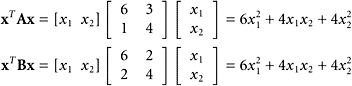
EXAMPLE 12
Illustrate Theorem 10 using the matrix in Example 11 by finding the symmetric matrix B that has the same quadratic form as the nonsymmetric matrix A.
SOLUTION With ![]() , we obtain
, we obtain
|
The quadratic forms are
 |
|
We have obtained equivalent quadratic forms!
EXAMPLE 13
Let ![]()
What is the quadratic form induced by this matrix? By a change of variables, show that the diagonal matrix D has the same quadratic form, with a different vector, as the quadratic form of the symmetric matrix B and nonsymmetric matrix A; namely,
|
SOLUTION Again, it is a straightforward calculation based on the definition:
|
We see a quadratic form in especially simple garb. There are no cross-product terms, such as y1y2. If we are willing to make a change of variables, such simple forms can always be found! We leave it to the reader to show that
|
by such a change of variables (see General Exercise 67).
Now we explain the important technique of simplifying a quadratic form arising from a symmetric matrix. Recall from Theorem 8 that every real and symmetric matrix A can be diagonalized by an orthogonal matrix:
|
where D is diagonal and U is an orthogonal matrix, UUT = I.
EXAMPLE 14
Let ![]()
Diagonalize the quadratic form that arises from this matrix.
SOLUTION The quadratic form involved here is
|
With a change of variables, we will obtain a diagonal matrix for the quadratic form. We find that the eigenvalues of B are 5 and 1. Furthermore, the corresponding eigenvectors, in normalized form, are the columns of the matrix
|
The matrix U is orthogonal: UUT = I. The change of variable needed here is x = Uy; namely, ![]() and
and ![]() . The effect on the quadratic form is then
. The effect on the quadratic form is then
|
In this equation, D is the diagonal matrix having the eigenvalues 1 and 5 on its diagonal.
EXAMPLE 15
What is the quadratic form induced by the matrix
|
Set the quadratic polynomial equal to a positive constant, such as 42. What is the corresponding geometric figure?
SOLUTION Clearly, we obtain:
|
Setting ![]() and dividing all terms by 42 produces the standard form of an ellipse,
and dividing all terms by 42 produces the standard form of an ellipse, ![]() . We shall have an ellipse for the graph. The semimajor axis is
. We shall have an ellipse for the graph. The semimajor axis is ![]() , and the semiminor axis is
, and the semiminor axis is ![]() . See Figure 8.1.
. See Figure 8.1.
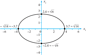
FIGURE 8.1 Ellipse ![]() .
.
EXAMPLE 16
If the term ![]() is changed to
is changed to ![]() in the equation of Example 15, what geometric figure emerges?
in the equation of Example 15, what geometric figure emerges?
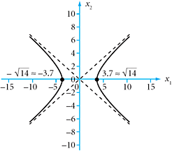
FIGURE 8.2 Hyperbola ![]() .
.
SOLUTION The equation now is ![]() If a large value is assigned to x1, we can satisfy the equation by choosing an appropriate large value for x2. The figure is therefore not bounded. In fact it is a hyperbola, having symmetry with respect to both the horizontal and vertical axes, and symmetry with respect to the origin. See Figure 8.2.
If a large value is assigned to x1, we can satisfy the equation by choosing an appropriate large value for x2. The figure is therefore not bounded. In fact it is a hyperbola, having symmetry with respect to both the horizontal and vertical axes, and symmetry with respect to the origin. See Figure 8.2.
Application: World Wide Web Searching
Beginning in 1998, Web search engines such as Google started to use the Web hyperlink structure to improve their search analysis. This is known as link analysis and it is based on fundamental linear algebra concepts. This approach resulted in remarkably accurate Web searches and it revolutionized the design of search engines!
Jon Kleinberg from Cornell University developed the HITS algorithm, which is a link analysis algorithm, during his postdoctoral studies at IBM Almaden. Dr. Kleinberg noticed a pattern among Web pages: Good hubs point to good authorities.
Pages with many outlinks serve as hubs or portal pages, whereas other pages with many inlinks are authorities on topics. All pages in the query list and all pages pointing to or from the query page are in a neighborhood set of the query list, which may contain anywhere from hundreds to hundreds of thousands of Web pages. The hub and authority scores are refined iteratively until they converge to stationary values. Let h and a be column vectors of hub and authority scores and let L be the adjacency matrix for the neighborhood set. It can be shown that
|
and, therefore, we obtain
|
Here LTL is the hub matrix and LLT is the authority matrix. Both of these are semidefinite matrices. From these equations, we see that the HITS algorithm is the power method applied to these matrices. It solves the eigenvalue problems
|
where λ1 is the largest eigenvalue of LTL (or LLT). The vectors a and h are the corresponding eigenvectors. There are many other important issues such as convergence, existence, uniqueness, and numerical computation of these scores that we leave to the reader to explore. Variations of the HITS algorithm have been suggested, each having advantages and disadvantages.
Google is based on the PageRank algorithm. It is a link–analysis algorithm, similar to the HITS algorithm, and involves a recursive scheme and the power method. Sergey Brin and Larry Page conceived of the PageRank algorithm and the Google system when they were computer science graduate students at Stanford University in 1998. Their original idea was that ‘‘a page is important if it is pointed to by other important pages.’’ The importance of a page is its PageRank score and it is determined by summing the PageRanks of all pages that point to this page. When an important page points to several pages, its weight (PageRank) is distributed proportionally.
The page rank is a measure of the importance of each Web page relative to all other Web pages in the World Wide Web. For each Web page, a ballot is taken among all Web pages with a hyperlink to that page counting as a vote for it. So the PageRank of a page is defined recursively and it depends on the number of incoming links and their PageRank metric. (The word ‘‘PageRank’’ is a pun on Larry Page’s name.) Although the exact details are a trade secret, the PageRank in the Google ToolBar goes from 0 to 10 using a logarithmic scale. Web pages have a high rank if they have many Web pages linked to them with high rank. Votes cast by important pages weigh more heavily and help to make other pages important.
For example, consider a small universe of four Web pages A, B, C, and D. If all these pages link to page A, then the PageRank of A, denoted pr(A), would be the sum of the PageRank of pages B, C, and D:
|
In addition, suppose that page B links to page C, whereas page D links to pages A, B, and C. Each page splits its vote over several pages. Page B gives half a vote to each of pages A and C. Page C gives one vote to page A. Page D gives one-third of a vote to pages A, B, and C. (See the sketch in Figure 8.3.) For each page that is linked to page A, its PageRank is divided by the total number of links from that page:
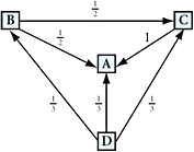
FIGURE 8.3 Web page links.
|
The actual PageRank formula incorporates two more considerations and is given by
|
For each Web page linked to A, its PageRank is divided by the number of links that come from that page. For example, ![]() (B) is the number of incoming links to page A from page B. The factor q (usually 0.85) is used to scale down indirect votes because direct votes are trusted more than indirect votes. To start off, all pages are given a small authority of 1 − q = 0.15, resulting in the property that the average PageRank of all pages will be 1. Google is constantly recalculating the PageRank of Web pages. When a PageRank tends to stabilize, it is used by a search engine. For additional details, see the online encyclopedia Wikipedia: en.wikipedia.org/wiki/PageRank
(B) is the number of incoming links to page A from page B. The factor q (usually 0.85) is used to scale down indirect votes because direct votes are trusted more than indirect votes. To start off, all pages are given a small authority of 1 − q = 0.15, resulting in the property that the average PageRank of all pages will be 1. Google is constantly recalculating the PageRank of Web pages. When a PageRank tends to stabilize, it is used by a search engine. For additional details, see the online encyclopedia Wikipedia: en.wikipedia.org/wiki/PageRank
Let ![]() be the PageRank row vector at the kth iteration, which can be written as
be the PageRank row vector at the kth iteration, which can be written as
|
where H is a row-normalized hyperlink matrix; that is, hij is nonzero if there is a link from page i to page j and is zero otherwise. Because of convergence problems such as cycling or dependence on the starting vector, the PageRank concept was revised to involve the power method applied to a primitive stochastic iteration matrix that always converges to the PageRank vector yT (a unique stationary distribution vector) independent of the starting vector. The asymptotic rate of convergence is governed by the magnitude of the subdominant eigenvalue λ2 of the transitive probability matrix. Google also uses nonmathematical metrics when responding to a query and is secretive about exactly what it does, but at the heart of the software is the PageRank algorithm.
Google’s algorithm for the ranking of Web pages uses a popularity contest style of search. Other iterative ranking methods predate Google’s PageRank algorithm by over seventy years. In his 1941 paper, Nobel Prize winning economist Wassily Leontief discussed an iterative method for ranking industries. In 1965, sociologist Charles Hubbell published an iterative method for ranking people. Computer scientist Jon Kleinberg developed the Hypertext Induced Topic algorithm for optimizing Web information and it was referenced by Google’s Sergey Brin and Larry Page. It has been said that ‘‘PageRank stands on the shoulders of giants!’’. For additional details on Web searching see Langville and Meyer [2005–2006] as well as Berry and Browne [2005].
Mathematical Software
Here is an example of using mathematical software to find the diagonalization of a complex matrix. Define the matrix
 |
|
How does one use mathematical software to find the diagonalization of this matrix?
We can use MATLAB, Maple, or Mathematica as follows:
|
|
|
|
The computer programs respond with A and the two new matrices P and D. The matrix equation PHAP = D should be true, and that is readily verified.
SUMMARY 8.1
• ![]()
This is the Standard Inner Product for ![]() .
.
• xyH is an n × n matrix of rank at most one (called the Outer Product)
• ![]() ,
, ![]() , and
, and ![]()
• ![]() and
and ![]()
•A = AH is the condition for a Hermitian matrix.
•A mapping f is self-adjoint if and only if ![]() .
.
• UHU = I is the condition for a square matrix to be unitary.
• UTU = I is the condition for a square real matrix to be orthogonal.
• x ![]() xTAx is the definition of a quadratic form in
xTAx is the definition of a quadratic form in ![]() .
.
• Theorems and Corollaries:
• Every self-adjoint mapping is linear.
• All eigenvalues of a self-adjoint operator are real.
• Any two eigenvectors of a self-adjoint operator are mutually orthogonal if they are associated with different eigenvalues.
• Eigenvalues of L and A are the same if A is the matrix for a linear transformation L relative to a given basis.
• The operator L is self-adjoint if its matrix satisfies A = AH.
• Spectral Theorem: Let L be a self-adjoint operator on an n-dimensional inner-product space, X. Then there exists an orthonormal basis {u1, u2, …, un} for X and a set of n real numbers λj such that L(uj) = λjuj, for 1 ≤ j ≤ n, and ![]() for all x ∈ X.
for all x ∈ X.
• Spectral Theorem, Matrix Version: If AH = A, then UHAU = D, where D is a diagonal matrix having the eigenvalues of A on its diagonal, and U is a unitary matrix whose columns are eigenvectors of A.
• If AH = A, then all eigenvalues of A are real.
• If A is real and AT = A, then all eigenvalues of A are real.
• If A is a real, symmetric matrix, then UTAU = D, where D is diagonal and U is orthogonal. The eigenvalues of A are on the diagonal of D.
• Cayley–Hamilton Theorem: If p is the characteristic polynomial of a matrix A, then p(A) = 0.
• If ![]() , then the quadratic forms of A and B are identical and B is symmetric.
, then the quadratic forms of A and B are identical and B is symmetric.
KEY CONCEPTS 8.1
Complex inner products, conjugate transpose, symmetric matrices, Hermitian matrices, self-adjoint transformations, spectral theorem, orthogonal matrices, unitary matrices, unitarily similar, diagonalization, Cayley–Hamilton Theorem, quadratic form, Web searching
GENERAL EXERCISES 8.1
1. Find the diagonalization of ![]()
2. Let ![]() ,
, ![]() and
and ![]() . Verify that {u, v, w} is orthonormal.
. Verify that {u, v, w} is orthonormal.
3. Find the eigenvalues of this matrix:
|
4. Find the successive powers of the matrices A and B given here, and discuss the negative integer powers also.
a. 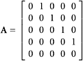
b. 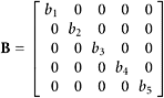
5. Can every orthogonal 2 × 2 matrix be put into the form ![]() for a suitable value of θ?
for a suitable value of θ?
6. Carry out the diagonalization of this self-adjoint matrix: ![]()
For encouragement along the way, we offer these guideposts: The eigenvalues are 1 and 4. The eigenvectors, before normalization, can be (1 + i, −1) and (1 + i, 2). For those eigenvectors the normalizing divisors are ![]() and
and ![]()
7. Let 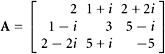
Without doing any calculation, conclude that the eigenvalues of this matrix are real.
8. Let ![]()
Explain the meaning of the assertion that A obeys the Cayley–Hamilton theorem. Verify the assertion.
9. Explain why the diagonal of a Hermitian matrix is real.
10. What are the graphs of xTAx = c, when ![]() and c is given different values such as c = −1, 0, 1?
and c is given different values such as c = −1, 0, 1?
11. Find all the matrices (symmetric and otherwise) that correspond to this quadratic form: ![]()
12. (Continuation.) With a change of variables, express the quadratic form in the preceding problem without the cross-product terms. Along the way, you should find eigenvalues ![]() .
.
13. Let ![]() where c is any real number. What are the eigenvalues and eigenvectors of A in terms of c?
where c is any real number. What are the eigenvalues and eigenvectors of A in terms of c?
14. What is A if its corresponding quadratic form is ![]()
15. Find all the matrices A such that
|
where α ≠ 0 and β ≠ 0.
16. Establish as true or find a counterexample to the assertion that the nonzero eigenvalues of a skew symmetric matrix are pure imaginary. The matrix A is skew symmetric if AT = −A.
17. Explain why an arbitrary square complex matrix is the sum of a Hermitian matrix and a skew Hermitian matrix. A matrix S is skew-Hermitian if SH = −S.
18. In the space ![]() consisting of all polynomials, use the inner product
consisting of all polynomials, use the inner product ![]()
![]() . Select a polynomial p, and define a linear operator L :
. Select a polynomial p, and define a linear operator L : ![]() →
→ ![]() by the formula L(x) = px. (This is the simple product of two polynomials: t
by the formula L(x) = px. (This is the simple product of two polynomials: t ![]() p(t)x(t).) Find the operator L* that has this property:
p(t)x(t).) Find the operator L* that has this property: ![]() . Assume that the polynomials can have complex coefficients, and that the variable t can be complex. The operator L* is called the adjoint of L and is a generalization of AH for matrices to operators for possible infinite-dimensional situations.
. Assume that the polynomials can have complex coefficients, and that the variable t can be complex. The operator L* is called the adjoint of L and is a generalization of AH for matrices to operators for possible infinite-dimensional situations.
19. Establish that for any m × n real matrix A, if Ax = 0 for all x in ![]() , then A = 0.
, then A = 0.
20. Explain why the columns of a square matrix must form an orthonormal set if the rows do so. Cite the crucial theorem from an earlier point in the book that justifies this.
21. (Continuation.) If the matrix in the preceding problem is not square, can we draw the same conclusion? A counterexample or a theorem is needed.
22. Establish directly that the eigenvalues of a real symmetric matrix are real and that the eigenvectors associated with different eigenvalues are mutually orthogonal.
23. A unitarily diagonalizable matrix A commutes with AH, which is called a normal matrix. Establish this fact.
24. If A is unitary, explain why A−1 and AH are also unitary. Is the product of two unitary matrices unitary? (Theorems or examples are needed.) Does the sum of two unitary matrices have any interesting properties? What useful property does the matrix ![]() have?
have?
25. Explain why ![]() , using only the definition of AH and the properties of an inner product.
, using only the definition of AH and the properties of an inner product.
26. Explain why an invertible matrix A satisfies the equation (AH)−1 = (A−1)H.
27. Let L be a self-adjoint operator on a finite-dimensional inner-product space (the scalar field being ![]() ). Let A be the matrix for L with respect to some basis. Is A necessarily symmetric? A theorem or example is needed.
). Let A be the matrix for L with respect to some basis. Is A necessarily symmetric? A theorem or example is needed.
28. Affirm that if we introduce a new inner product on ![]() by the equation
by the equation ![]() , then the transformation T defined by T(x1, x2) = (2x1+6x2, 4x1+7x2) is self-adjoint with respect to the new inner product.
, then the transformation T defined by T(x1, x2) = (2x1+6x2, 4x1+7x2) is self-adjoint with respect to the new inner product.
29. Let A be an n × n Hermitian matrix. Explain why this hypothesis leads to the conclusion that the map x ![]() Ax is self-adjoint on the space
Ax is self-adjoint on the space ![]() , with its standard inner product.
, with its standard inner product.
30. Let V be an inner-product space. Establish that the family of all self-adjoint operators from V to V is closed under addition and under multiplication by real scalars.
31. (Continuation.) In detail, establish that ![]() is self-adjoint and
is self-adjoint and ![]()
![]() is self-adjoint, where f1, f2, …,fn and g1, g2, …,gn are self-adjoint mappings from an inner-product space into itself and r1, r2, …,rm are real numbers.
is self-adjoint, where f1, f2, …,fn and g1, g2, …,gn are self-adjoint mappings from an inner-product space into itself and r1, r2, …,rm are real numbers.
32. Explain why the map ![]() is self-adjoint if and only if u = v.
is self-adjoint if and only if u = v.
33. Let {v1, v2, …, vm} be points in an inner-product space. Define ![]()
![]() , where r1, r2,…rn, are real numbers. Establish that T is self-adjoint.
, where r1, r2,…rn, are real numbers. Establish that T is self-adjoint.
34. In an inner-product space, let {u1, u2, …, un} and {v1, v2, …, vn} be linearly independent sets. Define a linear operator ![]() . Show that if ui = vi for 1 ≤ i ≤ n, then L is self-adjoint.
. Show that if ui = vi for 1 ≤ i ≤ n, then L is self-adjoint.
35. Let f be a mapping from ![]() into
into ![]() such that
such that ![]() for all x and y. Establish that there is a symmetric matrix A such that f(x) = Ax for all x and y.
for all x and y. Establish that there is a symmetric matrix A such that f(x) = Ax for all x and y.
36. Establish that if the matrix A is Hermitian, then the quadratic form ![]() is real valued. Assume that x ranges over the space
is real valued. Assume that x ranges over the space ![]() .
.
37. Affirm that if the real matrix A is orthogonally diagonalizable, then A must be symmetric. The hypothesis means that for some orthogonal matrix U, th ematrix UAUT is a diagonal matrix.
38. (Continuation.) Use the preceding problem and Theorem 8 to establish that if A and B are orthogonally diagonalizable, then the same is true of A + B.
39. Use the Cayley–Hamilton Theorem to get a formula for A−1 when A is invertible. Be sure to use somewhere in your work the hypothesis that A is invertible! You can assume that the characteristic equation of A is known.
40. Use the matrix A in Example 6. Find a formula for Ak by diagonalizing A. (Refer to Section 6.1), in particular, for this technique. The eigenvalues are 7 and 5. Then compute A2 by using the Cayley– Hamilton Theorem.
41. Explain why, for any n × n matrix A, An is in the span of {I, A, A2, …, An−1}.
42. Let q be any polynomial and A any square matrix. Verify that if λ is an eigenvalue of A, then q(λ) is an eigenvalue of q(A).
43. Establish that if n > 1, then there is no n × n matrix whose powers span ![]() .
.
44. Find out what n × n matrices have the property that An ∈ Span {A, A2, …, An−1}.
45. Explain, using induction, that for any n × n matrix A, Ak ∈ Span {A0, A1, …, An−1}for all nonnegative integers k.
46. Fix an n×n matrix A, and let matrices B and C be in the span of {A0, A1, A2,…}. Affirm that BC = CB.
47. Critique this proof of the Cayley–Hamilton Theorem. Let p(λ) = Det(A− λI). Therefore, we have p(A) = Det(A−AI) = Det(0) = 0. (See Barbeau [2000].)
48. Let A be a square matrix having possibly complex elements. Confirm that the diagonal of AAH has only nonnegative real numbers. Also, establish that AAH is Hermitian.
49. Explain why every 2 × 2 real matrix is similar to its transpose. Is this true for 2 × 2 complex matrices?
50. a. Find a 2 × 2 matrix, A, for which the dimension of Span {I, A}i s two. Then find other 2 × 2 matrices for which this dimension is zero and one, respectively.
b. Find a 3 × 3 matrix, A, for which the dimension of Span {I, A, A2} is three. Then find other 3 × 3 matrices for which this dimension is zero, one, and two, respectively.
c. Can you create examples of this sort for arbitrary n?
51. For z =(z1, z2, …,zn) ∈ ![]() , we use the notation
, we use the notation ![]() . Is the mapping
. Is the mapping ![]() linear?
linear?
52. If A is an n × n matrix, define S(A) to be the span of the nonnegative powers of A. This will be a subspace of ![]() . How many matrices A, B, C… are needed so that S(A), S(B), S(C)… spans
. How many matrices A, B, C… are needed so that S(A), S(B), S(C)… spans ![]() ?
?
53. Explain that if A is an m × n matrix of rank m, then AAT is invertible.
54. (Continuation.) Confirm that if A is an m × n matrix of rank m and B is an n × n invertible matrix, then ABBTAT is invertible. What about the case ABAT ?
55. Let A be a real matrix that is similar to a real diagonal matrix. Does it follow that A is symmetric? An example or theorem is needed.
56. Confirm that if ![]() for all x ∈
for all x ∈ ![]() , then u = v.
, then u = v.
57. In modern terms, explain the quote by Cayley on pp. 469–470. For additional information, see Midonic [1965, p. 198].
58. Can you find a 3 × 3 matrix whose powers span ![]() ?
?
59. Let A and B be n × n matrices such that 2A = B + BT. Does it follow that 2B = A + AT?
60. Using the matrix in Example 6, find the general expression for Ak as a single matrix.
61. We are g iven 
Find the explicit formula for the quadratic form induced by the matrix and show that it is a polynomial of degree two in three variables x1, x2, and x3.
62. Can the quadratic forms of the following matrices be expressed without the x1x2 term using changes of variables? Explain why or why not.
a. ![]()
b. ![]()
c. ![]()
63. Redo Example 13 using a direct change of variables.
64. Let C[−1, 1] be the vector space of all continuous real-valued functions defined on the closed interval [−1, 1]. Use the inner product ![]() . Define T on C[−1, 1] by the equation T(u) = wu, where w is a fixed function in C[−1, 1]. Is T self-adjoint?
. Define T on C[−1, 1] by the equation T(u) = wu, where w is a fixed function in C[−1, 1]. Is T self-adjoint?
65. (Continuation.) Use the definitions in the preceding problem, except that [T(u)](x) = (x2 + y2)u(y). Is T self-adjoint?
66. (Continuation.) Let V stand for the vector space of all polynomials p such that p(1) = p(−1) = 0. Use the inner-product of General Exercise 64. Establish that V is an inner-product space. Find out whether the operation of differentiation is self-adjoint. Define L as L(u) = u′ = du/dt.
67. Find the change of variables in Examples 12 and 13 so that xTAx = xTBx = yTDy.
68. (Adjacency Matrix.) In the figure, each of n = 15 nodes represents a Web page and a directed edge from node i to node j means that page i contains a Web link to page j. Construct the adjacency matrix A, which is an n × n matrix whose (i, j) entry is 1 if there is a link from node i to node j.
COMPUTER EXERCISES 8.1
1. For any matrix of the form ![]() , use mathematical software to find formulas for the factors in the equation A = QDQT, where QQT = I2 and D is diagonal.
, use mathematical software to find formulas for the factors in the equation A = QDQT, where QQT = I2 and D is diagonal.
2. Determine numerically whether these matrices are Hermitian or skew-Hermitian:
a. 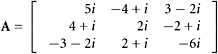
b. 
3. Determine numerically whether these matrices are orthogonal or unitary:
a. 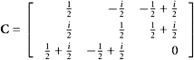
b. 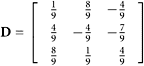
4. Let 
Determine numerically the values of a, b, and c so that this matrix is orthogonal.
5. Let ![]()
Determine the general form of a real 2 × 2 orthogonal matrix.
6. Let ![]()
Establish that a general 2 × 2 normal matrix is either symmetric or the sum of a scalar matrix and a skew-symmetric matrix. Note: Amatrix A is a normal matrix if AAT = ATA when A is real or if AAH = AHA when A is complex.
7. (Continuation.) Establish that each of these are normal matrices:
a. real symmetric matrices
b. real orthogonal matrices
c. complex Hermitian matrices
d. complex unitary matrices
8. Consider
 |
|
For the matrix A shown, compute its eigenvalues and eigenvectors as well as the unitary matrix U such that UHAU = D.
9. Consider
 |
|
Compute the diagonalization of matrix B.
10. Consider
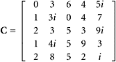 |
|
Verify that the matrix C obeys the Cayley-Hamilton Theorem.
11. Consider
 |
|
For the given matrix, compute the symmetric matrix ![]() . Show that the corresponding quadratic forms are equivalent.
. Show that the corresponding quadratic forms are equivalent.