CHAPTER SIX
Eigensystems
6.1 EIGENVALUES AND EIGENVECTORS
The purpose of computing is insight, not numbers.
—RICHARD W. HAMMING (1915–1998)
Numbers are intellectual witnesses that belong only to mankind.
—HONORE DE BALZAC (1799–1850)
Introduction
Sometimes, the effect of multiplying a vector by a matrix is to produce simply a scalar multiple of that vector. For example,
|
We often want to know to what extent this phenomenon occurs for a given matrix. That is, we ask for all instances of the equation Ax = λx, where A is given but we know neither the vector x nor the scalar λ. Because there are two unknowns on the right multiplied together, this is not a linear problem! If λ were fixed, and we only wanted to find all the appropriate x-vectors, it would be a standard linear problem. Even easier is the case when x is known, and we only want to determine λ. Each of these is a linear problem. But it is nonlinear if x and λ are both unknown. Therefore, we must expect to encounter some obstacles in solving this problem.
Eigenvectors and Eigenvalues
First, we notice that the vector 0 always solves the equation Ax = λx. We rule out that case as uninteresting. The properly posed question is therefore: For what scalars λ is there a nontrivial solution (x ≠ 0) to the equation
|
where the matrix A is given and the vector x is sought? This is known as the eigenvalue problem for the given matrix, A.
DEFINITION
Let A be any square matrix, real or complex. A number λ is an eigenvalue of A if the equation
|
is true for some nonzero vector x. (Here λ is allowed to be a real or complex number.) The vector x is an eigenvector associated with the eigenvalue λ. The eigenvector may also be complex.
Arithmetic with complex numbers cannot be avoided in the subject of eigenvalues. That is why the preceding definition explicitly allows for complex numbers to enter our calculations. See Appendix B for a summary of complex arithmetic.
In matrix theory, some terminology has changed over time. For example, eigenvalues have been known as characteristic values, latent roots, and eigenwerte. As recently as 1949, the eminent mathematician D. E. Littlewood was calling an eigenvalue a “latent root,” an eigenvector a “pole,” and the inverse of a matrix its “reciprocal,” as well as using ![]() as the “norm” of the vector x = (x1, x2, …, xn), which is not the standard definition given in Section 7.1. (See The Skeleton Key of Mathematics by Littlewood [2002].) The German word “eigen” has several different English translations, such as proper, peculiar, and strange. Many German idioms contain this word.
as the “norm” of the vector x = (x1, x2, …, xn), which is not the standard definition given in Section 7.1. (See The Skeleton Key of Mathematics by Littlewood [2002].) The German word “eigen” has several different English translations, such as proper, peculiar, and strange. Many German idioms contain this word.
EXAMPLE 1
Illustrate the use of these new terms eigenvalue and eigenvector by using the equation above.
SOLUTION That equation has the form Ax = λx, where
|
Thus, 5 is an eigenvalue of the given matrix A, and a corresponding eigenvector is [1, 1]T.
We must be prepared for complex eigenvalues and eigenvectors, even if A is real. Notice that if λ is an eigenvalue of A and if x and y are eigenvectors of A associated with λ, then x + y (if not 0) is also an eigenvector associated with λ. A similar observation applies to cx for any nonzero scalar c. (Verify this!) Hence for fixed A and λ, the set {x : Ax = λx} is a subspace. It will often be the subspace containing only the vector, 0, as happens when λ is not an eigenvalue of A.
Using Determinants in Finding Eigenvalues
If λ is an eigenvalue of A, then the equation Ax = λx has a nontrivial solution. Consequently, the equation (A − λI)x = 0 has a nontrivial solution, and the matrix A − λI is noninvertible. Hence, we have Det(A − λI) = 0. Because the argument is reversible, we have this result:
THEOREM 1
A scalar λ is an eigenvalue of a matrix A if and only if Det(A − λI) = 0.
The effect of this theorem is to turn the intractable nonlinear problem (with unknowns λ and x) into a problem involving only λ. Conceptually this is very important, although finding the correct values of λ may still be numerically challenging.
The equation Det(Ax − λI) = 0 is called the characteristic equation of A. It is the equation from which we can compute the eigenvalues of A. The function λ ![]() Det(A − λI) is the characteristic polynomial of A.
Det(A − λI) is the characteristic polynomial of A.
EXAMPLE 2
What are the characteristic equation and the eigenvalues of the matrix ![]() ? For each eigenvalue, find an eigenvector.
? For each eigenvalue, find an eigenvector.
SOLUTION To answer this, we set up the matrix equation
|
Next, we expand the determinant and obtain:
|
This leads to λ2 − λ − 6 = 0, or (λ − 3)(λ + 2) = 0. Hence, the given matrix A has precisely two eigenvalues: 3 and −2. Along the way one gets the characteristic polynomial, λ ![]() λ2 − λ − 6.
λ2 − λ − 6.
Flushed with success we pursue the eigenvectors. First, let λ = 3. The homogeneous equation that we must solve is then
|
Notice that the matrix in this subproblem is noninvertible. We expect that, because λ has been chosen to satisfy the equation Det(A − λI) = 0, and that is the same as making A− λI noninvertible. (Recall Theorem 5 in Section 4.1.) Row reduction of the augmented matrix leads to
|
We obtain x1 − x2 = 0. The simplest eigenvector for the eigenvalue 3 is therefore u = (1, 1).*
In the same way, we let λ = −2 and search for a vector in the null space of the matrix
|
We obtain 4x1 + x2 = 0. A convenient eigenvector is then v = (1, −4). We now know that Au = 3u and Av = −2v. Can there be any other eigenvalues for this matrix? No, any eigenvalue would necessarily satisfy the equations we arrived at, and there were no more than two eigenvalues.

SOLUTION The characteristic equation is, by definition,
 |
|
The steps involved in getting the values of λ are as follows:
 |
|
Our work indicates that the eigenvalues are −2, 1, 3, and 7. (Typical eigenvalues in the real world are not integers!) Now, select an eigenvalue, say 3, and search for a corresponding eigenvector. We must solve (A − 3I)x = 0 with a nonzero vector x. This is a homogeneous problem whose augmented matrix is
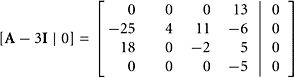 |
|
The solution is u = (2, −37, 18, 0). This can be verified in a separate calculation. Namely, Au = (6, −111, 54, 0) = 3u, and this indeed is 3 times u.
Linear Transformations
The concepts of eigenvalues and eigenvectors carry over to linear transformations.
DEFINITION
Let L be a linear operator mapping a vector space V into itself. If
|
then we call λ an eigenvalue and v an eigenvector of the linear operator L.
For example, let L(v) = v″, where V is the vector space of twice-differentiable functions on the symmetric interval [−π, π]. Since d(sin t)/dt = cos t and d(cos t)/dt = −sin t, −1 is an eigenvalue and the sine function is an eigenvector.
In Example 2, the pertinent conclusions can be conveyed as follows:
|
|
The matrix containing two eigenvectors as columns is denoted by P, and the diagonal matrix on the right is denoted by D. Thus, we have AP = PD. In this case, one can take another step and write P−1AP = D or A = PDP−1. This is possible because P in this case is invertible. For some other examples, this step is not permitted because P is singular. In the terminology of Section 5.3, the equation A = PDP−1 indicates that our original matrix A is similar to the diagonal matrix D. Remember that similar is a highly technical term in matrix theory, meaning in this context that A = PDP−1.
DEFINITION
A matrix A is diagonalizable if there is a diagonal matrix D and an invertible matrix P such that
|
We repeat that there is a profound difference between the two equations AP = PD and P−1AP = D. The latter equation requires that P be invertible. Although we can always arrive at an equation of the form AP = PD, we may be unable to proceed to P−1AP = D. Obviously, the invertibility (nonsingularity) of the matrix P is the issue. (Notice that the equation AP = PD is always solvable, since P = 0 is one solution. Therefore, this case must be ruled out.) The next example illustrates what may happen.
EXAMPLE 4
Find the eigenvalues and eigenvectors of the matrix
|
Carry out the diagonalization process, if possible.
SOLUTION To find the eigenvalues, write
|
There is only one eigenvalue—namely, λ = 1. When we look for an eigenvector, we solve the homogeneous equation having augmented matrix
|
One possible eigenvector is (1, 0). All others are multiples of this one. We can, of course, write AP = PD, which looks like this:
|
The matrix P is noninvertible and A is not diagonalizable! We do not have enough eigenvectors to provide a basis for ![]() .
.
In computing the eigenvalues of a matrix, we may encounter repeated roots (multiple roots) in the characteristic polynomial. As mentioned previously, the multiplicity of an eigenvalue as a root of the characteristic polynomial is called its algebraic multiplicity. The dimension of the accompanying eigenspace is termed the geometric multiplicity of that eigenvalue. These can differ, but the algebraic multiplicity is always greater than or equal to the geometric multiplicity. Example 4 exhibits this phenomenon in a 2 × 2 matrix. The eigenvalue 1 has algebraic multiplicity two, because the factor (λ − 1) occurred twice in the characteristic polynomial λ ![]() Det(A−λI). Also, we say that the eigenvalue has geometric multiplicity one, since it leads to a one-dimensional subspace of eigenvectors.
Det(A−λI). Also, we say that the eigenvalue has geometric multiplicity one, since it leads to a one-dimensional subspace of eigenvectors.
For a formal definition of these two concepts, let A be an n × n matrix. Let its characteristic polynomial be
|
In this equation some factors can be repeated; that is, they can occur more than once. The complex numbers λj are the eigenvalues of A. If a certain factor λ − λj occurs kj times in the factorization, the corresponding eigenvalue has algebraic multiplicity kj. If the corresponding subspace has dimension ![]() j, then we say that the eigenvalue has geometric multiplicity
j, then we say that the eigenvalue has geometric multiplicity ![]() j. This means that
j. This means that ![]() j is the dimension of Null(A − λjI). The following theorem is given without proof; it asserts that kj ≥
j is the dimension of Null(A − λjI). The following theorem is given without proof; it asserts that kj ≥ ![]() j.
j.
THEOREM 2
The geometric multiplicity of an eigenvalue cannot exceed its algebraic multiplicity.
Distinct Eigenvalues
When all the eigenvalues of a matrix are different, the associated eigenvectors form a linearly independent set, according to the following theorem.
THEOREM 3
Any set of eigenvectors corresponding to distinct eigenvalues of a matrix is linearly independent.
PROOF Let Ax(i) = λix(i) for 1 ≤ i ≤ k. Assume that the vectors x(i) are nonzero and that the eigenvalues λi are all different from each other. We hope to establish that the set {x(1), x(2), …, x(k)} is linearly independent. Our proof will be by the method of contradiction. Suppose that {x(1), x(2), …, x(k)} is linearly dependent. By Theorem 9 in Section 2.4, some element of this ordered set is a linear combination of the preceding elements in the set. Let j be the first integer such that x(j+1) is a linear combination of x(1), x(2), …, x(j). Then the set {x(1), x(2), …, x(j)} is linearly independent, and j < k. We carry out the following steps:
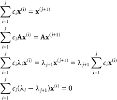 |
|
By the linear independence of {x(1), x(2), …, x(j)}, the coefficients ci(λi − λj+1) are all zero. Because the eigenvalues are distinct, we conclude that all ci are zero. Hence, by a preceding equation, x(j+1) = 0. This cannot be true. (All the eigenvectors are nonzero.) This contradiction concludes the proof.
Another, slightly different, proof can be given as follows.
PROOF Let Ax(i) = λix(i), for 1 ≤ i ≤ k, where all x(i) are nonzero and the eigenvalues are distinct. Let r be the largest index for which {x(1), x(2), …, x(r)} is linearly independent. If r = k, we are finished. Assume, therefore, that r < k. Then {x(1), x(2), …, x(r+1)} is linearly dependent. It follows that x(r+1) is in the span of {x(1), x(2), …, x(r)}. Thus, we obtain ![]() , where the coefficients ai are not all zero because x(r+1) ≠ 0. Now compute a few things:
, where the coefficients ai are not all zero because x(r+1) ≠ 0. Now compute a few things:
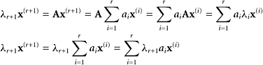 |
|
By subtraction between the two preceding equations, we get ![]() . None of the factors λi − λr+1 are zero, by hypothesis. Also, the coefficients ai are not all zero. We have here a contradiction of the linear independence of {x(1), x(2), …, x(r)}.
. None of the factors λi − λr+1 are zero, by hypothesis. Also, the coefficients ai are not all zero. We have here a contradiction of the linear independence of {x(1), x(2), …, x(r)}.
The preceding theorem is valid if we define eigenvalues and eigenvectors for any linear transformation, T. No finite-dimensionality assumption is required. A slight rewording of the proof would be needed: At first, the equation T(x(α)) = λαx(α) would be assumed, where α runs over some index set. If the set of x(α) is linearly dependent, we can then pass to a finite linearly dependent set, as in the proof of Theorem 3.
Because of its practical importance, we state an immediate consequence of Theorem 3:
COROLLARY 1
If an n × n matrix A has n distinct eigenvalues, then A is diagonalizable.
Bases of Eigenvectors
If an n × n matrix A is given, there may or may not exist a basis for ![]() consisting of eigenvectors of A. For example, we can find a basis for
consisting of eigenvectors of A. For example, we can find a basis for ![]() consisting of eigenvectors of the matrix
consisting of eigenvectors of the matrix ![]() . Because A is triangular, the eigenvalues are λ1 = 3 and λ2 = 7. The eigenvalue–eigenvector pairs are
. Because A is triangular, the eigenvalues are λ1 = 3 and λ2 = 7. The eigenvalue–eigenvector pairs are ![]() and
and ![]() . Hence for
. Hence for ![]() , there is a basis for
, there is a basis for ![]() made up of eigenvectors:
made up of eigenvectors: ![]() .
.
However, for ![]() , 0 is the only eigenvalue (a repeated root in the characteristic polynomial λ
, 0 is the only eigenvalue (a repeated root in the characteristic polynomial λ ![]() λ2). There is only a one-dimensional eigenspace—namely, the span of
λ2). There is only a one-dimensional eigenspace—namely, the span of ![]() .
.
Finally, for ![]() , 0 is again the only eigenvalue (repeated), but there are two free variables in this case. Here there is a basis for
, 0 is again the only eigenvalue (repeated), but there are two free variables in this case. Here there is a basis for ![]() consisting of eigenvectors of C—namely,
consisting of eigenvectors of C—namely, ![]() and
and ![]() .
.
COROLLARY 2
If an n × n real matrix A has n distinct real eigenvalues, then the corresponding eigenvectors of A constitute a basis for ![]() .
.
If A has repeated eigenvalues, no conclusion can be drawn without further analysis!
Application: Powers of a Matrix
The factorization of a matrix
|
discussed previously can be used to compute efficiently the powers of A. Let us see how this works by starting with A2. Assume as known the equation A = PDP−1. Multiply both sides of this equation on the left by A, getting
|
(Notice how the associative law for matrix multiplication enters this calculation.) This argument can be repeated, with the result that
|
This is easy to compute, because the powers of a diagonal matrix are also diagonal, and the diagonal entries are powers of the diagonal elements in D. In algebraic form, this is
 |
|
EXAMPLE 5
Using the matrices from Example 2, compute Ak.
SOLUTION From the equation A = PDP−1, we get Ak = PDkP−1 or
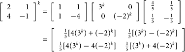 |
|
We obtain a quick verification by letting k = 1.
Characteristic Equation and Characteristic Polynomial
In the general case of an n × n matrix, the function p defined by
|
will be a polynomial of degree n in the variable λ. As we know, it is called the characteristic polynomial of A. When we set it equal to zero, the result is called the characteristic equation. This polynomial may have n different roots, or there may be repeated roots. Repeated roots occur when the characteristic polynomial has factors of the form (λ − λj)k, where k > 1. The characteristic polynomial may have complex roots, as we now illustrate.
EXAMPLE 6
Let ![]()
Find the eigenvalues of A by using the characteristic polynomial.
SOLUTION Proceeding as before, we get
|
The roots of this polynomial are computed with the quadratic formula. Recall that the quadratic equation aλ2 + bλ + c = 0 has roots
|
For the case at hand, we obtain
|
Notice that a real matrix may have complex eigenvalues.
Diagonalization Involving Complex Numbers
The diagonalization of matrices involving complex eigenvalues and eigenvectors is illustrated in the next example.
SOLUTION In principle, this is worked out in the way we have already illustrated in the real case. But now we must undertake some arithmetic calculations with complex numbers. (See Appendix B.) Start with the eigenvalue λ1 = 2 + i. For this value of λ, we have
|
If our work is correct, this matrix will be noninvertible. Looking at the second column, we conclude that row 2 should be (1 − i) times row 1. We verify this:
|
Hence, suitable row operations (which we need not carry out!) will lead us to
|
Let x be a nonzero solution to this homogeneous system of equations. Let x2 be the free variable, so that we obtain (1 + i)x1 = x2. Letting x2 = 1 + i, we get x1 = 1, and a convenient eigenvector is then [1, 1 + i]T. Proceeding in the same way with the eigenvalue λ2 = 2 − i, we arrive at the matrix
|
Again, this must be noninvertible. Just for amusement, we check this noninvertibility property by computing the determinant, which should be zero:
|
Hence, suitable row operations (which again need not be performed) will reduce the matrix:
|
We obtain x2 = (1 − i)x1, where x1 is a free variable. By letting x1 = 1, we obtain a convenient solution to the homogeneous system of equations x = [1, 1 − i]T. The P-matrix is then
|
Computing the inverse of P in the usual way leads to
|
The diagonalization equation, A = PDP−1, is then
 |
|
Notice in Examples 6 and 7 that both the eigenvalues and the eigenvectors occur as complex conjugate pairs. The reason for this is that the matrix A is real but the eigenvalues and eigenvectors are complex. When A is real and Ax = λx, it follows that ![]() .
.
THEOREM 4
If A is a real matrix and has a complex eigenvalue λ, then the conjugate ![]() is also an eigenvalue. Thus, we have Ax = λx and
is also an eigenvalue. Thus, we have Ax = λx and ![]() .
.
Of course, if a real matrix does not have any complex eigenvalues, then there are no complex conjugate pairs!
Application: Dynamical Systems
Here we return to the computation of Akx for high values of k. (We shall see in Examples 8 and 9 how this problem arises in simple dynamical systems.) Start with an eigenvector and eigenvalue for A, say
|
Then
|
We can repeat this process to obtain A3v = λ3v, and so on. In general, we have
|
Thus, for any positive integer k, it is easy to compute Akv when v is an eigenvector of A. If A is an n × n matrix, and if we have a basis for ![]() consisting of eigenvectors of A, then we can compute Akx for any x with relative ease, as follows. Let {v(1), v(2), …, v(n)} be a basis for
consisting of eigenvectors of A, then we can compute Akx for any x with relative ease, as follows. Let {v(1), v(2), …, v(n)} be a basis for ![]() consisting of eigenvectors of A. Suppose explicitly that
consisting of eigenvectors of A. Suppose explicitly that
|
Given any x in ![]() , first express x in terms of the basis:
, first express x in terms of the basis: ![]() . Then multiply by Ak, getting
. Then multiply by Ak, getting
|
No powers of A need be computed, and that advantage is worth noting for future applications. (See Example 8.)
If the eigenvalues and eigenvectors of A are not available, the powers of A can be computed in the usual way. Remember that multiplying two n × n matrices involves roughly n3 arithmetic operations, and therefore computing Ak is costly if carried out simply by repeated multiplications. For studying the long-term behavior of a dynamical system, one can compute ![]() efficiently by repeated squaring:
efficiently by repeated squaring:
|
EXAMPLE 8
A dynamical system is modeled by the equation x(k) = Ax(k−1), where
|
For any starting point, x(0), this equation defines an infinite sequence of vectors in ![]() . What is the long-term behavior of this system if the starting vector is x(0) = (6.97, 3.87)?
. What is the long-term behavior of this system if the starting vector is x(0) = (6.97, 3.87)?
SOLUTION To answer this, we can use mathematical software and brute force by repeatedly carrying out matrix–vector multiplications x(k) = Ax(k−1) starting with x(0) = (6.97, 3.87). We plot these points in Figure 6.1 using the symbol *.

FIGURE 6.1 A trajectory of the dynamical system in Example 8.
The next step is to express the starting vector x(0) = ( 6.97, 3.87) as a linear combination of the eigenvectors. First, using mathematical software, we obtain the matrix D of eigenvalues and matrix V of eigenvectors:
|
Because the eigenvectors are the columns of V, we must solve Vc = x(0) for c. Because both V and c are known, this 2 × 2 system can be solved directly or by using mathematical software to find c = (−6.6981, −1.4947). Hence, we obtain
|
Next, we derive the formulas suitable for computing any x(k) in an efficient manner.
 |
|
The vectors x(k) eventually settle down in the direction of v(2), because the component in the direction of v(1) is diminishing quickly. The magnitude of the vectors is increasing because of the factor (1.0732)k.
For comparison purposes, Figure 6.1 shows two sets of points: the repeated matrix–vector multiplication (marked with the * symbol) and the dominant-term approximation (marked with the + symbol). The latter appears to lie on a straight line because the dominant eigenvalue term overwhelms any effect from the other eigenvalues.
Where the points appear to lie on a straight line, it is because the term involving the dominant eigenvalue overwhelms the effect of the other eigenvalue.
EXAMPLE 9
A dynamical system is given in the form x(1) = Ax(0), x(2) = Ax(1), etc., where
|
Discover the long-term behavior of this system.
SOLUTION We use mathematical software to generate the sequence x(1), x(2), and soon, up to x(30). We use commands similar to those in Example 8 except that A and x(0) are different.
In an example like this, it is easy to continue this sequence of vectors x(k). Figure 6.2 shows that the points are following an orbit that spirals around the origin at ever-increasing distances. To find a dominant-term approximation for the successive points, we would follow a procedure similar to the one in Example 8. Again, we can use mathematical software to compute the eigenvalues and eigenvectors of A. The eigenvalues are 1.08 ± 0.229i, and the matrix of eigenvectors can be taken to be ![]() .
.

FIGURE 6.2 A spiral trajectory of the dynamical system in Example 9.
Further Dynamical Systems in 
We describe the geometrical behavior of some simple dynamical systems having the form
|
If the points on one trajectory approach a point, that point is called an attractor or a sink. If the points on a trajectory move away from a point, then such a point is a repeller or a source. If points on some trajectory move toward a point and then move away from the point, that point is a saddle point. Also, a trajectory can cycle by repeating with a certain period, or spiral about a point (inward or outward).
Suppose that A is the simple matrix
|
The eigenvalue–eigenvector pairs are a, (1, 0) and b, (0, 1). We have
 |
|
Depending on the values of the elements a, b of the matrix A and of the starting vector x(0) = (c1, c2), we obtain various behaviors for the dynamical system.
If x(0) = (1, 1), then x(k) = (ak, bk). If 0 < a < 1 and 0 < b < 1, then x(k) → (0, 0) and the origin is an attractor. If 0 < a < 1 and b > 1, then x(k) → (0, ∞), and the origin is a repeller along the x2-axis. If a > 1 and 0 < b < 1, then x(k) → (∞, 0), and the origin is a repeller along the x1-axis. If a > 1 and b > 1, then x(k) → (∞, ∞), and the origin is a repeller.
Analysis of a Dynamical System
Here are the steps in analyzing a discrete dynamical system, such as
|
where A and x(0) are prescribed, and A is n × n.
1. Observe that
|
2. Find the eigenvalues λ1, λ2, …, λn of A.
3. Order the eigenvalues according to magnitude: |λ1| > |λ2| ≥ ··· ≥ |λn|.
4. Find eigenvectors, one for each eigenvalue, say v(1), v(2), …, v(n). Thus, we have
|
5. To proceed, we must assume that the initial vector, x(0), is in the span of the set of eigenvectors. Thus, we write
|
for suitable coefficients cj. Compute these coefficients.
6. Now there is a simple formula for computing the vectors x(k) in the dynamical system:
|
7. For isolating the dominant term in the preceding equation, we can write
|
This equation shows the influence of λ1 on the sequence of vectors x(0), x(1), x(2), …. The factors (λj/λ1) are all at most 1 in absolute value.
Application: Economic Models
Here, we consider an application of linear algebra in the science of economics. It is not unreasonable to expect linear algebra to play a role in analyzing the economy, since, at first glance, causes and effects seem to have a linear relation. For example, if the input to an industry is doubled, one expects the output to double as well.
The economic model discussed here assumes that the economy of a country is divided into a number of industries. The term industry is interpreted broadly: not only do we have the coal industry and the steel industry, but we also have the medical industry, the education industry, the government industry, and so forth. The word sectors can also be used in this context.
Suppose we have n of these industries. A realistic model may require a rather large value of n—say n = 500 or 10,000. Each industry produces in one year a product having a certain total value. Let us say that the value of the output from industry i, in one year, is xi dollars. We choose the letter xi, because it will be an unknown quantity. Why should the value of the year’s output from an industry be unknown? It is because the value is determined by the price at which the output is sold, and that price is, to some extent, free to be manipulated by the various industries in the model.
The ith industry will consume a certain fraction of each industry’s output in a year, including its own output. For example, the electric industry (whose product is electricity) will consume some outputs from the coal industry, the natural gas industry, and others. It will probably consume some of its own product.
In general, let aij be the fraction of the total yearly production from industry j used by industry i in one year. Thus, in row i of the matrix A being constructed, the needs of industry i are listed. These numbers represent the fractions of each industry’s yearly output that are needed by industry i in carrying out its role in the economy.
We assume that all the yearly output from each industry is bought by the industries being considered in our model. Hence, each column sum, ![]() , must equal 1. That sum accounts for the entire output of industry j going back to the various industries in our model.
, must equal 1. That sum accounts for the entire output of industry j going back to the various industries in our model.
Conversely, the row sums are restricted only by nonnegativity.
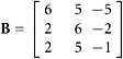
EXAMPLE 10
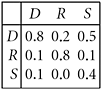
Explain this concrete case involving three industries, called E, C, and S (perhaps standing for electricity, coal, and steel).
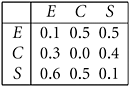
SOLUTION This table shows that the output of industry E goes one-tenth to E, three-tenths to C, and six-tenths to S, totaling 1.0. It also shows that industry E needs one-tenth of the output of industry E, five-tenths of the output from industry C, and five-tenths of the output from industry S. Each row and column have similar interpretations. Notice that the column sums are all unity, reflecting the fact that everything has to go somewhere.
In the general model, industry i purchases fractions ai1, ai2, …, ain of the outputs from industries 1, 2, …, n. Because xj is the value of the total output from industry j, the total yearly cost incurred by industry i in one year is
|
In a state of equilibrium, the earnings of each industry would equal its expenditures. This means that ![]() . This is a system of equations having the form x = Ax. Hence, A must have 1 as one of its eigenvalues! (There is no interest in the solution x = 0.)
. This is a system of equations having the form x = Ax. Hence, A must have 1 as one of its eigenvalues! (There is no interest in the solution x = 0.)
THEOREM 5
If each column of a square matrix A sums to 1, then 1 is an eigenvalue of A, and the system Ax = x has a nontrivial solution.
PROOF The hypothesis can be stated in the form ![]() for all j. This means that the vector u = (1, 1, …, 1) is an eigenvector of AT corresponding to the eigenvalue 1 of AT. But, by General Exercise 32, A and AT have the same eigenvalues. Hence, 1 is an eigenvalue of A.
for all j. This means that the vector u = (1, 1, …, 1) is an eigenvector of AT corresponding to the eigenvalue 1 of AT. But, by General Exercise 32, A and AT have the same eigenvalues. Hence, 1 is an eigenvalue of A.
In the language of economics, Theorem 1 asserts that there exists a set of prices for the commodities such that each industry has an income that equals its costs. These special prices are called equilibrium prices. Because this equilibrium price vector x is an eigenvector of the matrix A, all multiples of it are also equilibrium price vectors. Thus, if each industry decides to double its prices, there will still be equilibrium. In this discussion, we think of xi as the price, or the declared value of the yearly output of an industry.
EXAMPLE 11
The problem x = Ax is to be solved nontrivially, using the matrix from Example 10.
SOLUTION We have
 |
|
We can use the integer solution [70, 51, 75]T for the homogeneous system of equations.
Application: Systems of Linear Differential Equations
Let x = [x1, x2, …, xn]. Each xi is interpreted as a function of a variable t. Often, t is time in a concrete problem. The notation ![]() signifies the derivative of xi with respect to t, and it is therefore a rate of change in the variable xi. Naturally, we write
signifies the derivative of xi with respect to t, and it is therefore a rate of change in the variable xi. Naturally, we write
|
Now let A be an n × n matrix. A system of n linear differential equations with n variables then can be written simply as x′ = Ax. The ith equation in this system is
|
For a down-to-earth numerical example, we can take
|
Here we see two simple differential equations, but neither can be solved alone, since the righthand sides involve both x1 and x2. Does it help to know that the eigenvalues of A are 5 and −4? At first glance there seems to be no connection between the system of first-order differential equations and the eigenvalues of A. However, we shall use the eigenvalues of A to produce solutions of the system of differential equations. Even at this stage we can enunciate a general theorem—that is, one that is valid for any n.
THEOREM 6
If Au = λu, then the function t ![]() eλtu is a solution of the differential equation x′ = Ax.
eλtu is a solution of the differential equation x′ = Ax.
PROOF The proof is trivial if u = 0. In the other case, u ≠ 0 and we have a genuine eigenvalue and eigenvector. In the differential equation x′ = Ax, we replace x by eλtu, getting A(eλtu) = λeλtu. Now cancel the positive scalar eλt, leaving Au = λu, which is true.
Returning to the 2 × 2 numerical example, we find that the eigenvalues of A are 5 and −4. Corresponding eigenvectors are v = [1, 1] and w = [2, −7]. Therefore, the functions t ![]() e5tv and t
e5tv and t ![]() e−4t w are solutions of the previous 2 × 2 system. By linearity, a more general solution is
e−4t w are solutions of the previous 2 × 2 system. By linearity, a more general solution is
|
What recourse do we have for solving x′ = Ax when A is diagonalizable? This term refers to the factorization A = P−1DP, in which D is a diagonal matrix. The differential equation is now x′ = P−1DPx or Px′ = DPx. Letting y = Px, we have a familiar sort of problem: y′ = Dy. After solving this problem for y, we get x from the equation x = P−1y.
There is much more to the theory, and the reader can pursue this topic in books such as Sadun [2001], Nobel and Daniel [1988], and Mirsky [1990].
Epilogue: Eigensystems without Determinants
Many professional mathematicians advocate a separation of the subject of eigenvalues from determinant theory. This view of the subject is backed by the knowledge gained from numerical analysis, where determinants are almost never used. (They are not competitive with other algorithms in speed and accuracy.) Here, we give one example showing how determinants can be banished from eigenvalue theory. The following theorem and proof are adapted from the paper by Axler [1995], cited in the references.
THEOREM 7
Every linear operator defined on and taking values in a finite-dimensional vector space has at least one eigenvalue.
PROOF Let L be such an operator, and let u be a nonzero vector in the domain of L. The sequence {u, L(u), L2(u), …} cannot be linearly independent because the space involved here is finite dimensional. Thus, there must exist a nontrivial relationship ![]() . Let p be the polynomial defined by the equation
. Let p be the polynomial defined by the equation ![]() . Thus, we have p(L)u = 0. By the Fundamental Theorem of Algebra (Appendix B), this polynomial has roots (zeros) in the complex plane. (This is a deep theorem, and it would not be true if we insisted on real-valued roots.) These roots lead to a factored form for p; namely, p(t) = c(t − r1)(t − r2)···(t − rn). Now we have
. Thus, we have p(L)u = 0. By the Fundamental Theorem of Algebra (Appendix B), this polynomial has roots (zeros) in the complex plane. (This is a deep theorem, and it would not be true if we insisted on real-valued roots.) These roots lead to a factored form for p; namely, p(t) = c(t − r1)(t − r2)···(t − rn). Now we have
|
If each factor L − riI were injective, p(L)u could not be 0, since we started with the nonzero vector u. Thus, for some value of i, L − riI is not injective, and we have a nonzero solution to the equation L(x) − rix = 0.
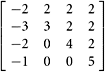
EXAMPLE 12
The process used in the preceding proof can be illustrated in a concrete case. Let the linear transformation be L(x) = Ax, where
 |
|
Find an eigenvalue of A by the method used in the proof of Theorem 7.
SOLUTION We select any nonzero vector for u, such as u = [1, 2, 3]T. With the help of mathematical software, we find that
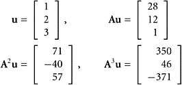 |
|
We need go no further because the four points listed form a linearly dependent set. (Why?) Create a matrix B whose columns are the four vectors already constructed. By row reduction we can find a linear combination of the columns of B that is zero, in a nontrivial manner:
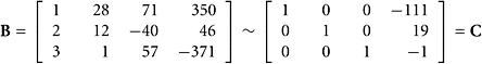 |
|
The systems Bx = 0 and Cx = 0 have the same solutions, and we can set the free variable equal to 1, thereby getting x = [111, −19, 1, 1]T. At this stage we know that
|
Defining the polynomial p by the equation p(t) = 111 − 19t + t2 + t3, we can write p(A)u = 0. Now we need the roots of the polynomial p. In MATLAB, one defines a polynomial by giving its coefficients: p = [1, 1, -19, 111]. Then the roots are obtained with the command r = roots(p). They are
|
Then
|
In this example, it turns out that each factor A − rkI is not injective, and r1, r2, and r3 are all eigenvalues of A.
Mathematical Software
In Example 1, we can use mathematical software to verify the results. Here is a summary of the basic commands available in three well-known mathematical software systems:
|
|
|
|
|
|
We find that the matrix has two eigenvalues, 5 and 7.
In Example 2, we can check our results using mathematical software.
|
|
|
|
|
|
MATLAB returns the eigenvalues 3 and −2 with eigenvectors (0.7071, 0.7071) and (−0.2425, 0.9701), These are correct because they are scalar multiples of the simple eigenvectors u = (1, 1) and v = (1, −4) already known. In Maple and Mathematica, we obtain similar results but the eigenvector corresponding to the eigenvalue −2 has been scaled to (![]() , 1) and (−1, 4), respectively.
, 1) and (−1, 4), respectively.
In Example 4, matrix A is diagonalizable and can be written in the form A = PDP−1. As we noted previously, this equation contains an abundance of information! To begin with, the columns of P are eigenvectors of A. Furthermore, the diagonal elements of the diagonal matrix D are the eigenvalues of A. All of this additional information about A is hard-won, although mathematical software seems to do it effortlessly. Here are the procedures to get eigenvalues and eigenvectors for a matrix using common mathematical software packages:
MATLAB returns the repeated eigenvalue 1 with eigenvectors (1, 0) and (−1, 0). The equation AP = PD is essentially correct, but there is some roundoff error of magnitude 10−15. Results from Maple and Mathematica are similar.
In Example 6, we can find the roots of the characteristic polynomial using either MATLAB, Maple, or Mathematica:
|
|
|
|
The results from all of these mathematical software systems are the same.
Again, in Example 7, we can verify the results using mathematical software:
|
|
|
|
MATLAB returns eigenvalues 2 ± i and eigenvectors (0.40821 ± 0.40821i, 0.8165), which can be normalized to agree with the preceding results. With Maple and Mathematica we obtain similar results within roundoff error.
In Example 8, we have used the following MATLAB commands:
|
|
These points are plotted in Figure 6.1 and marked with the symbol *. We can also apply the analysis that leads to the dominant term. The following MATLAB code computes the points x(j) and plots them in Figure 6.1 using the + symbol.
|
|
In Example 8, we can compute the long-term behavior of these points in a more efficient way. First, we compute eigenvalues and eigenvectors for the matrix A. The commands are as follows:
|
|
We display the matrices V and D from MATLAB; they turn out to be
|
Remember, MATLAB rounds numbers for display. The full-precision values are stored, however, and can be seen by using the command format long. The columns of the matrix V are normalized eigenvectors of A, and the diagonal elements of D are the eigenvalues, listed in the same order as the eigenvectors. (A vector is normalized by dividing it by its length, and the length of a vector x in ![]() is
is ![]() . These matters are explained in Section 7.1.) We can verify the work by computing AV − VD, which should be the 0-matrix. In this example with MATLAB, this matrix turns out to be
. These matters are explained in Section 7.1.) We can verify the work by computing AV − VD, which should be the 0-matrix. In this example with MATLAB, this matrix turns out to be
|
and that is “close enough for government work.”
SUMMARY 6.1
• Let A be an n × n matrix. A number λ is an eigenvalue of A if the equation Ax = λx is true for some nonzero vector x. Then the vector x is an eigenvector associated with the eigenvalue λ. (Here the eigenvalue and eigenvector may be complex.)
• The polynomial p(λ) = Det(A − λI) of degree n in the variable λ is the characteristic polynomial of A, and Det(A − λI) = 0 is the characteristic equation.
• The characteristic polynomial has the form ![]() , where k1 + k2 + k3 + ··· + km = n. Each eigenvalue λj has algebraic multiplicity kj and if Dim(Null (A − λjI)) =
, where k1 + k2 + k3 + ··· + km = n. Each eigenvalue λj has algebraic multiplicity kj and if Dim(Null (A − λjI)) = ![]() j, then the geometric multiplicity is
j, then the geometric multiplicity is ![]() j. Moreover, kj ≥
j. Moreover, kj ≥ ![]() j.
j.
• If A = PDP−1, then Ak = PDkP−1 and this is true for any invertible P. If D is a diagonal matrix, then ![]() for k ≥ 1.
for k ≥ 1.
• Suppose that the dynamical system x(k) = Ax(k−1) has eigenvalues of A that are ordered |λ1| > |λ2| ≥ ··· ≥ |λn| and eigenvectors v(1), v(2), …, v(n). Express the given initial vector as ![]() for suitable coefficients cj. Then the dominant term is
for suitable coefficients cj. Then the dominant term is ![]() .
.
• Theorems and Corollaries:
• If L(v) = λv and v ≠ 0, then λ is an eigenvalue and v is an eigenvector of the linear operator defined on any vector space.
• A is diagonalizable if the equation P−1AP = D is true, where D is a diagonal matrix and P is an invertible matrix.
• A scalar λ is an eigenvalue of a matrix A if and only if Det(A − λI) = 0.
• The geometric multiplicity of an eigenvalue cannot exceed its algebraic multiplicity.
• Any set of eigenvectors corresponding to distinct eigenvalues of a matrix is linearly independent.
• If an n×n matrix has n distinct eigenvalues, then it is diagonalizable.
• Every polynomial of degree 1 or more has a root in the complex field.
• If each column of a square matrix A sums to 1, then 1 is an eigenvalue of A, and the system Ax = x has a nontrivial solution.
• Every linear operator defined on and taking values in a finite-dimensional vector space has at least one eigenvalue.
KEY CONCEPTS 6.1
Eigenvalues and eigenvectors for matrices and linear transformations, diagonalizable, basis of eigenvectors, powers of a matrix, characteristic polynomial, characteristic equation, dynamical systems, economic models, eigensystems without determinants
GENERAL EXERCISES 6.1
1. What are the eigenvalues of these matrices:
|
Show the calculations for the matrix B and, if possible, check your answers using MATLAB or similar software.
2. Carry out the diagonalization of matrices:
|

Find the eigenvalues and eigenvectors of A. (Assume abc ≠ 0.)
4. Let ![]()
Find the eigenvalue–eigenvector pairs. Explore the geometric effect of letting x(k) = Ax(k−1) and k = 0, 1, 2, ….
5. The matrix ![]() represents a rotation of 90° counterclockwise. Obviously, Ax is never a simple multiple of x (if x ≠ 0), because the vectors x and Ax point in different directions. However, the equation Ax = λx must have nontrivial solutions because the characteristic polynomial must have roots. Explain this apparent contradiction. Also, find the diagonalization of A and check your work.
represents a rotation of 90° counterclockwise. Obviously, Ax is never a simple multiple of x (if x ≠ 0), because the vectors x and Ax point in different directions. However, the equation Ax = λx must have nontrivial solutions because the characteristic polynomial must have roots. Explain this apparent contradiction. Also, find the diagonalization of A and check your work.
6. Find the diagonalization of ![]()
Check your work.
7. Show why the conjugate of a + ib is not necessarily a − ib. (Give some examples.)
8. Find the eigenvalues of 
9. Find a basis for ![]() consisting of eigenvectors of the matrix
consisting of eigenvectors of the matrix ![]()
10. Criticize this argument: With a sequence of row operations, we establish that
 |
|
Therefore, the eigenvalues of A are 1, 3, and −122.
11. By examining the column sums, prove that 3 is an eigenvalue of the matrix
 |
|
12. (Practice with complex numbers.) Find the real and imaginary parts of these complex numbers:
a. (5 + 2i)(3 − 4i)
b. (5 + 2i)/(3 − 4i)
c. (5 + 2i)/|3 − 4i|
d. (3 − 5i)(2 + i)/(4 + 3i)
13. Find all the values of λ for which this equation has nontrivial solutions:
|
14. For what values of α will the matrix
|
have real eigenvalues?
15. Find the eigenvalues of ![]()
For each eigenvalue, find an eigenvector. Find a nonzero matrix P such that AP = PD, where D is a diagonal matrix. Give D explicitly. Verify your work with independent calculations.
16. Let 
Find all the eigenvalues of A. For each eigenvalue, find an eigenvector.
17. Let ![]()
Find the characteristic polynomial. Find the eigenvalues. Find an eigenvector for each eigenvalue. Find a matrix P such that P−1AP is a diagonal matrix.
18. Let 
Find the eigenvalues of A. Find the eigenspaces for A. Give the algebraic and geometric multiplicities of the eigenvalues. Find matrices P and D that make the equation AP = PD nontrivially true. Here D should be a 3 × 3 diagonal matrix, with the eigenvalues on its diagonal. Also, P should be a 3 × 3 matrix. Note: We are not claiming that P is invertible. There can be many answers for P.
19. In Example 3, find an eigenvector corresponding to the eigenvalue 7.
20. (Continuation.) What is the diagonalization of the matrix in the preceding exercise?
21. Let ![]()
where a and b are arbitrary real numbers.
a. Find the eigenvalue–eigenvector pairs.
b. Show that ![]() where
where ![]() and θ is the angle in the triangle at the origin in the complex plane with sides a, b, and hypotenuse r.
and θ is the angle in the triangle at the origin in the complex plane with sides a, b, and hypotenuse r.
c. Discuss the geometric effect of the iteration x(k) = Ax(k−1). Suppose that 0 < a < 1, 0 < b < 1, and a2 + b2 = 1.
d. Verify numerically your conclusions using a = 0.6 and b = 0.8.
22. Let ![]() , where a, b, c, and d are arbitrary real numbers.
, where a, b, c, and d are arbitrary real numbers.
a. Establish that the eigenvalues of the matrix A are ![]() .
.
b. Find the necessary and sufficient condition on the matrix A in order that it have two different eigenvalues. Find the eigenvectors.
c. Explain why A has only one eigenvalue if (a − d)2 = −4bc. What are the eigenvectors in this case? Hint: You may use mathematical software such as Maple to do the symbolic manipulations.
23. (Continuation.)
a. Find the necessary and sufficient conditions on the matrix ![]() in order that its eigenvalues be real. Assume that the entries in the matrix are real numbers.
in order that its eigenvalues be real. Assume that the entries in the matrix are real numbers.
b. Explain why the eigenvalues of A are real if bc ≥ 0.
c. Using your results, establish that a symmetric 2 × 2 matrix must have real eigenvalues.
24. (Continuation.) Find the necessary and sufficient conditions on the matrix ![]() in order that its eigenvalues be complex. (Remember that the numbers a, b, c, and d are real.)
in order that its eigenvalues be complex. (Remember that the numbers a, b, c, and d are real.)
25. (Continuation.)
a. Find the necessary and sufficient condition on the matrix ![]() in order that it not be diagonalizable.
in order that it not be diagonalizable.
b. Explain what happens when a = d and bc ≠ 0.
26. Assume that A is a 2 × 2 matrix whose elements are integers. Find the necessary and sufficient conditions on the entries of the matrix in order that the eigenvalues of A be integers.
27. Find all the 2 × 2 matrices that have 1 as one of their eigenvalues.
28. Find all the 2 × 2 matrices that have eigenvalues 3 and 7.
29. Explain why a square matrix is invertible if and only if 0 is not one of its eigenvalues.
30. Let A be an n × n matrix whose rows all sum to the same value. What can you say about eigenvalues and eigenvectors of A?
31. Establish that if A is invertible and if λ is an eigenvalue of A, then λ−1 is an eigenvalue of A−1.
32. Argue that the eigenvalues of a matrix A are also eigenvalues of AT. Do A and AT have the same characteristic polynomial? (Explain why or give a counterexample.)
33. Verify that similar matrices (as defined in Section 5.3.) have the same eigenvalues.
34. Substantiate that if an n × n matrix has n different eigenvalues, then the matrix is diagonalizable.
35. Consider a dynamical system where
|
Explain why the sum of the two components of x(r) is a constant; that is, is independent of r. (Here each x(r) is a vector in ![]() .)
.)
36. Let A be an upper triangular matrix whose diagonal elements are all different from one another. Establish that if B is invertible, then BAB−1 is diagonalizable.
37. Explain why the hypothesis {u1, u2, …, un} is a linearly independent set in ![]() leads to the conclusion that there is an n × n invertible matrix A having the vectors ui as eigenvectors. Can the eigenvalues also be assigned freely?
leads to the conclusion that there is an n × n invertible matrix A having the vectors ui as eigenvectors. Can the eigenvalues also be assigned freely?
38. All eigenvalues are real for a symmetric matrix (A = AT). Explain why and give some numerical examples.
39. All eigenvalues are purely imaginary or zero for a skew-symmetric matrix (A = −AT). Explain why and give some examples.
40. Argue that if the n × n matrix A has n different real eigenvalues, then there is a basis for ![]() consisting of eigenvectors of A.
consisting of eigenvectors of A.
41. For each of these 2 × 2 matrices, find its eigenvalues and eigenvectors as well as the algebraic multiplicity of the eigenvalues and geometric multiplicity of the eigenvectors.
a. ![]()
b. ![]()
c. ![]()
d. ![]()
e. ![]()
f. ![]()
g. ![]()
42. There are sixteen 2 × 2 matrices with elements from the set {0, 1}. How many of these matrices do not have eigenvalues from the same set? What are these matrices and their eigenvalues?
43. Let λ be an eigenvalue of an n × n matrix A, and define V = {x : Ax = λx}. This set is called an eigenspace of A. Establish in detail that V is a subspace of ![]() . Is each vector in V an eigenvector of A?
. Is each vector in V an eigenvector of A?
44.
a. In Figure 6.1, some of the points arising from the dynamical system in Example 8 are shown. How can we plot a curve instead of a finite set of points in this example? There may be many answers. Find the best one.
b. In Figure 6.2, some of the points arising from the dynamical system in Example 9 are shown. How can we plot a curve instead of a finite set of points in this example? There may be many answers. Find the best one.
45. If possible, find a 2 × 2 matrix for which the corresponding dynamical system has these three initial points: x(0) = (1, 1), x(1) = (3, 0), and x(2) = (3, −3).
46. Find the eigenvalues and eigenvectors of these matrices:
a. 
b. 
c. 
d. 
47. Establish that the eigenvalues of a triangular matrix are the numbers on its diagonal. Explain why the eigenvalues of a matrix cannot be computed by first using row-reduction techniques to get a triangular matrix, and then reading off the diagonal elements.
48. Explain why ![]() . Here, Diag(d1, d2, …, dn) is the diagonal matrix having the given numbers on its diagonal.
. Here, Diag(d1, d2, …, dn) is the diagonal matrix having the given numbers on its diagonal.
49. Let ![]() for a2 + b2 ≥ c2.
for a2 + b2 ≥ c2.
Show that the eigenvalues of A are real.
50. Let ![]() where a ≠ c and b ≠ 0.
where a ≠ c and b ≠ 0.
Determine Ak and verify for k = 1, 2, 3, 4.
51. If A2 = 0, what are the eigenvalues of A? Assume A ≠ 0.
52. Affirm that if AP = PD, where D is a diagonal matrix, and P is invertible, then the columns of P are eigenvectors of A and the diagonal elements of D are eigenvalues of A.
53. Confirm that if A is any n × n matrix, then its characteristic polynomial has as its term of highest degree ±λn.
54. Let {u1, u2} be a linearly independent pair of vectors in ![]() . Let arbitrary real numbers λ1 and λ2 be given. Does there necessarily exist a 2 × 2 matrix A such that Aui = λiui for i = 1, 2?
. Let arbitrary real numbers λ1 and λ2 be given. Does there necessarily exist a 2 × 2 matrix A such that Aui = λiui for i = 1, 2?
55. The generalized eigenvalue problem asks for the values of λ for which A − λB is noninvertible. To begin with, prove that AV = BVD where V is a full matrix with columns containing the generalized eigenvectors and D is a diagonal matrix containing the generalized eigenvalues on the main diagonal. Recall that for the eigenvalue exercise AV = VD. (For a fixed pair of matrices, the set{A − λB : λ ∈ ![]() } is called a pencil of matrices.)
} is called a pencil of matrices.)
56. (Continuation.) If B is invertible, then the generalized eigenvalue problem described in the preceding exercise can be turned into the equivalent ordinary eigenvalue exercise: Det(B−1 A − λI) = 0. Verify this assertion. Use this procedure to find the eigenvalues λ that make A − λB noninvertible, when ![]() and
and ![]()
57. (Continuation.) Solve the generalized eigenvalue problem A = λB, where
|
Here, one expects only to make A − λB noninvertible. Repeat for ![]()
58. In Example 8, we discarded a term that eventually became negligible. This was the term −6.6981(.7268)k. The retained (dominant) term was −1.4947(1.0732)k. For what values of k will the dominant term be greater than 10 times the negligible term?
59. Let A and B be diagonal matrices of the same size. Find a simple formula for AB and its inverse, if it has one.
60. (Micro-Research Project.) In a dynamical system of the type considered in this section, we have an equation x(k) = Ax(k−1) and a starting value x(0). How can we estimate the sensitivity of x(200) to small changes in x(0)?
61. In the dynamical systems of Examples 8 and 9, explain why successive points become farther apart as they recede from the origin.
62. Explain why or find a counterexample: Every 2 × 2 matrix is similar to its transpose.
63. Refer to Example 8 and Figure 6.1. Does the curve have two asymptotes? If so, find the formulas for the asymptotes and explain the phenomenon.
64. Let A be an n × n matrix, all of whose rows are the same. Find two eigenvalues of A.
65. (Micro-Research Project.) Can a two-dimensional dynamical system produce points lying on a circle? Answer the same question for an ellipse, a parabola, and a hyperbola.
66. Explain why if A = PBP−1, then Ak = PBkP−1 for k = 1, 2, 3, ….
67. We know that every square matrix has an eigenvalue and a corresponding nonzero eigenvector. The simplest example of a linear transformation that has no eigenvalues is outlined here. Let ![]() be the vector space of all polynomials. Define a linear transformation L by the equation (Lp)(t) = tp(t). Complete the argument by assuming that L has an eigenvalue and a corresponding nonzero eigenvector.
be the vector space of all polynomials. Define a linear transformation L by the equation (Lp)(t) = tp(t). Complete the argument by assuming that L has an eigenvalue and a corresponding nonzero eigenvector.
68. All eigenvalues have absolute value one for an orthogonal matrix (AAT = I). Explain why and give some examples.
69. Let A be an n × n matrix, and let u = [1, 1, 1, …, 1]T. If AT u = u, then the equation Ax = x has a nontrivial solution. Explain.
70. Let 
Find all the eigenvalues. Find all the eigenvectors. What are the algebraic and geometric multiplicities? Find the matrices such that AP = PD, where D is a diagonal matrix. Determine the matrices in the diagonalization factorization A = PDP−1. Give a general formula for Ak.
71. In Example 7, find the diagonalization equation A = PDP−1, when the order of the entries in the diagonal matrix D is reversed.
72. Suppose x and y are eigenvectors of A associated with λ. Explain why all ax + by, for scalars a and b except when ax + by = 0, are eigenvectors associated with λ.
73. All eigenvalues are positive for a positive definite matrix: xT Ax > 0 for all x ≠ 0. Explain why and give some numerical examples.
74. Show that the Fibonacci sequence x0 = 0, x1 = 1, and xk+1 = xk + xk−1 for k ≥ 1 can be written as
|
where ![]()
Determine Ak.
75. In Example 5, verify the results for k = 2 and k = 3.
76. In Example 7, find an expression for Ak as a single matrix and verify that it is correct for k = 1 and 2.
77. Let A be an n × n real matrix, where n is odd. Explain why A must have at least one real eigenvalue.
COMPUTER EXERCISES 6.1
1. Let 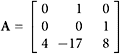 ,
, 

For each of these three matrices, determine the eigenvalues and eigenvectors. Find the diagonal matrix containing the eigenvalues. Find the matrix whose columns are unit eigenvectors. Verify the equation A = PDP−1 and the two similar equations for B. In verifying the answers (if you are using MATLAB) first use the command format long to get the values to 15-digit accuracy from that point on. Use the eigenvalue test to determine whether any of these three matrices are noninvertible. How do you account for the fact that the eigenvalues are integers? Is that phenomenon to be expected whenever the given matrix has integer entries?
2. Using the matrix  study the dynamical system defined by the equations x(0) = (1, 1, 1) and x(k+1) = Ax(k).
a. Are the successive points tending to lie on a line? If so, what is the equation of the line (in ![]() )? You will need the eigenvalues and eigenvectors of A to answer these questions.
)? You will need the eigenvalues and eigenvectors of A to answer these questions.
b. Can this dynamical system be run backward to get x(−1), x(−2) and so forth? If so, give the formula by which we compute x(i−1) from x(i), where i = 0, −1, −2, ….
c. Also run the system backward to find out the long-term behavior in the negative direction. Probably 30 or 40 steps will suggest the ultimate behavior in both cases (forward and backward).
3. Write programs in MATLAB, Maple, and Mathematica for Example 5 involving powers of a matrix. Verify the results by carrying out the calculation with matrix–matrix multiplications and by using the formula derived.
4. Write programs for Example 9 and compare the results of (1) repeated matrix–vector multiplication and of (2) an analysis involving just the dominant term. Plot the results.
5. Use Maple or Mathematica to compute the eigenvalues of a general matrix ![]() . Show that these results agree with your direct algebraic calculations done by hand.
. Show that these results agree with your direct algebraic calculations done by hand.
6. (Continuation.) Use Maple or Mathematica to compute the eigenvectors of a general matrix ![]() of order two. Show that these results agree with your direct algebraic calculations done by hand.
of order two. Show that these results agree with your direct algebraic calculations done by hand.
7. Political affiliations change from one generation to the next. We consider three parties, labeled D, R, and S (not necessarily Democrats, Republicans, and Socialists). The following table shows how party membership shifts from one generation to the next. For example, membership in S goes 40% to S, 10% to R, and 50% to D in one generation. What is the long-term outlook for the three parties?
8. Carry out the complete analysis of the dynamical system in Example 9. Find the eigenvalues and eigenvectors. Express the terms in the dynamical system in the manner of Example 8. When does x(k) enter the fourth quadrant? Solve this analytically, if possible (that is, not experimentally). This is rather difficult. You may find the Euler equation helpful: x + iy = reiθ, where r = |x + iy| and eiθ = cos θ + i sin θ.
9. Suppose that a dynamical system is governed by the equation x(k) = Ax(k−1), for k = 1, 2, …., where the parameter k is often measured in discrete units (seconds, hours, days, years, etc.). Usually, we are interested in letting t → ∞. However, if A is invertible, we can let t go to −∞. The equation x(k) = Ax(k−1) becomes x(k−1) = A−1x(k), and we let k = 0, −1, −2, …. This simple idea opens the possibility of seeing into the past. Carry out this strategy on the system in Example 9.
10. Compute the eigenvalues and eigenvectors of these matrices:


11. For the following matrices A, plot the trajectories for the dynamical systems x(k+1) = Ax(k) using a variety of different values for the starting point x(0):
a. ![]()
b. ![]()
c. ![]()
12. For the following matrices A, plot the trajectories for the dynamical systems x(k+1) = Ax(k) starting with x(0) = (4, 4):
a. ![]()
b. ![]()
If a real 2 × 2 matrix A has complex eigenvalues λ = a ± bi, then the trajectories of the dynamical system x(k+1) = Ax(k) lie on a closed orbit if |λ| = 1 (0 is an orbital center); spiral inward if |λ| < 1 (0 is a spiral attractor); spiral outward if |λ| > 1 (0 is a spiral repeller).
13. Using mathematical software in Example 12, find all the eigenvalues and eigenvectors to show that they agree with the results given in the text. What are the algebraic and geometric multiplicities?
14. By repeating Examples 8 and 9 on your computer system, reproduce the plots in Figures 6.1 and 6.2.