2.4 GENERAL VECTOR SPACES
Mathematics is a game played according to certain simple rules and meaningless marks on paper.
—DAVID HILBERT (1862–1943)
When you try to prove a theorem, you don’t just list the hypotheses, and start to reason. What you do is trial and error, experimentation, guesswork.
—PAUL R. HALMOS (1916–2006)
Vector Spaces
There are many vector spaces other than the spaces ![]() that we have been using heretofore. What type of mathematical constructs will be called “vector spaces”? The structure they must have is set out in the following formal definition.
that we have been using heretofore. What type of mathematical constructs will be called “vector spaces”? The structure they must have is set out in the following formal definition.
DEFINITION
A vector space is a set V of elements (called vectors), together with two algebraic operations, called vector addition and scalar multiplication. The following axioms must be fulfilled:
1. If u and v are vectors, then u + v is defined and is an element of V.
(Closure axiom for addition)
2. For all u and v in V, u + v = v + u.
(Commutativity of vector addition)
3. For any three vectors u, v, and w, (u + v) + w = u + (v + w).
(Associativity of vector addition)
4. There is an element 0 in V such that for all u in V, u + 0 = u.
(Existence of a zero vector)
5. For each vector u there is at least one element ![]() in V such that
in V such that ![]() + u = 0.
+ u = 0.
(Existence of additive inverses)
6. If u is a vector and is a scalar, then the product αu is defined and is an element of V.
(Closure axiom for scalar–vector product)
7. For any scalar α and vectors u and v, α(u + v) = αu + αv.
(Distributive law: scalar times vectors)
8. If α and β are scalars and u is a vector, then (α + β)u = αu + βu.
(Distributive law: scalar sum times a vector)
9. If α and β are scalars and u is a vector, α(βu) = (αβ)u.
(Associativity of scalar–vector product)
10. For each u in V, 1 · u = u.
(Multiplication of unit scalar times vector)
The reader will notice that these requirements are exactly the salient properties of the spaces ![]() that we called attention to in Section 2.1.
that we called attention to in Section 2.1.
We have already noticed that, with the definitions adopted in Section 2.1, ![]() is a vector space. Thus, we have at once an infinite number of different vector spaces, because n can be any natural number.
is a vector space. Thus, we have at once an infinite number of different vector spaces, because n can be any natural number.
The word scalar occurs frequently in the context of vector spaces. It almost always will mean a real number, but in some situations there is good reason for allowing complex numbers as scalars. (A complex number is of the form α + iβ, where α and β are real numbers and i2 = −1. See Appendix B.)
It turns out that the element ![]() in Axiom 5 is unique for each vector u. It is usually denoted by −u. The axiom then states that (−u) + u = 0 for all u. We further drop the parentheses and use Axiom 2 in this last equation to arrive at u − u = 0.
in Axiom 5 is unique for each vector u. It is usually denoted by −u. The axiom then states that (−u) + u = 0 for all u. We further drop the parentheses and use Axiom 2 in this last equation to arrive at u − u = 0.
Theorems on Vector Spaces
To illustrate the deductions that can be drawn from the preceding axioms, we consider five theorems valid in all vector spaces. We can use only the axioms to prove Theorem 1. But then we can use the axioms and Theorem 1 to prove Theorem 2, and so on.
THEOREM 1
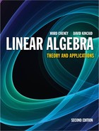
In any vector space, if c is a scalar, then c0 = 0.
PROOF Let x = c0. We want to prove that x = 0.
 |
|
See General Exercise 19 for another proof of Theorem 1.
THEOREM 2
In a vector space, if x is a vector and c is a scalar such that cx = 0, then either c = 0 or x = 0.
PROOF Assume the hypotheses, and suppose that c ≠ 0. Then c−1 exists, and we can multiply the equation cx = 0 by c−1, arriving at 1 · x = c−10. By Theorem 1 and Axiom 10, this becomes x = 0.
THEOREM 3
In a vector space, for each x, the point ![]() is uniquely determined.
is uniquely determined.
PROOF The crucial property of ![]() is that
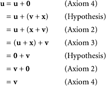
is that ![]() + x = 0. Suppose, then, that for some x we have both u + x = 0 and v + x = 0. Can we conclude that u must equal v? It is probably not obvious, but one proof goes like this:
+ x = 0. Suppose, then, that for some x we have both u + x = 0 and v + x = 0. Can we conclude that u must equal v? It is probably not obvious, but one proof goes like this:
 |
|
Notice that in this proof each equality requires specific justification and the axioms are used in the order indicated.
THEOREM 4
In a vector space, every vector x satisfies the equation 0x = 0.
PROOF One proof proceeds as follows, and the axioms used are indicated in each step.
 |
|
Verify the use of the axioms in the order indicated.
THEOREM 5
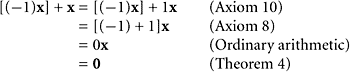
In any vector space, we have (−1)x = ![]() .
.
PROOF Following the proof above, we have
 |
|
Consequently ![]() = (−1)x by Theorem 3.
= (−1)x by Theorem 3.
Before going on, some remarks should be made. First, the element ![]() is written as −x or (−1)x. Theorem 5 justifies this. Second, the structure that is described by the ten axioms is technically a real vector space. This means that the constants appearing in Axioms 6–10 are real numbers. The real numbers in this context are often called scalars to distinguish them from the elements of V, which are then called vectors. (Thus, the answer to the question “What is a vector?” can be given truthfully as “It is an element of avectorspace.”)
is written as −x or (−1)x. Theorem 5 justifies this. Second, the structure that is described by the ten axioms is technically a real vector space. This means that the constants appearing in Axioms 6–10 are real numbers. The real numbers in this context are often called scalars to distinguish them from the elements of V, which are then called vectors. (Thus, the answer to the question “What is a vector?” can be given truthfully as “It is an element of avectorspace.”)
Later in the book, we shall broaden our perspective and discuss vector spaces with complex numbers as the scalars. Certain problems in vector space theory (notably eigenvalue problems) may have no solution if we restrict ourselves to the real numbers as scalars. When one speaks of a real vector space, it means only that the scalars are taken to be real numbers. In principle, other fields can be used for the scalars. If a particular field, F, is used, one speaks of a vector space over the field F. For information about fields, consult a textbook on abstract algebra or search the World Wide Web on the Internet.
Various Examples
We present a number of examples to illustrate these concepts.
EXAMPLE 1
Is the set of all polynomials having degree no greater than 3 a vector space?
SOLUTION Some elementary polynomials are p0(t) = 1, p1(t) = t, p2(t) = t2, and p3(t) = t3. Notice that any polynomial of degree at most 3 is a linear combination of the four polynomials p0, p1, p2, and p3. Thus, we can write
|
The set we have described is a vector space—it being assumed that the usual algebraic operations are used. One can add two polynomials of degree at most 3, and the result is another polynomial of degree at most 3. The zero element in this vector space is the polynomial defined by p(t) = 0 for all t. Notice that the notation p2 is the name of the function whose value at t is given by p2(t) = t2. One should not refer to t2 as a polynomial. It is nothing but a real number, because t is understood to be a real number. The notation t ![]() t2 can also be used to specify the function p2. We do not stop to verify all the vector-space axioms for this vector space. (They are very easy.)
t2 can also be used to specify the function p2. We do not stop to verify all the vector-space axioms for this vector space. (They are very easy.)
In the same way as in Example 1, for each nonnegative integer n, we have a space consisting of all polynomials of degree not exceeding n. This space is usually written ![]() . Now we have two infinite lists of distinct vector spaces,
. Now we have two infinite lists of distinct vector spaces, ![]() and
and ![]() , where n = 1, 2, 3, ….
, where n = 1, 2, 3, ….
EXAMPLE 2
Consider the set of all continuous real-valued functions defined on the interval [−1, 1]. Is this a vector space if we adopt the standard definitions for the algebraic operations?
|
SOLUTION Why is the first axiom true in this space? If we add two continuous functions, the result is another continuous function, by a theorem in calculus. A similar remark concerns the multiplication of a continuous function by a scalar. Thus, the two closure axioms are true by some theorems in calculus. The remaining axioms are all easily verified.
The space in Example 2 is customarily given the designation C[−1, 1]. More properly, one should write C([−1, 1]), because for an arbitrary domain, D, we would write C(D). As in Example 1, one should make a careful distinction between a function f and one of its values, f(t). In this book, we try to adhere to these standards, and the reader is encouraged to do the same.
EXAMPLE 3
Consider the set of all infinite sequences
|
If we use the natural definitions of vector addition and scalar multiplication, is this a vector space?
SOLUTION Yes. The closure axioms are true, just as they are for ![]() . In fact, we have here an obvious extension of those familiar spaces. This new space should be named
. In fact, we have here an obvious extension of those familiar spaces. This new space should be named ![]() . Notice that a sequence x is really a function. Its domain is the set of natural numbers,
. Notice that a sequence x is really a function. Its domain is the set of natural numbers, ![]() = {1, 2, 3,…}. We could use either the notation x(k) or xk or xk for a generic component of the vector x. In set theory, this space would also be denoted by
= {1, 2, 3,…}. We could use either the notation x(k) or xk or xk for a generic component of the vector x. In set theory, this space would also be denoted by ![]() . (In general, the set of all functions from one set B into another set A is denoted by AB. For example,
. (In general, the set of all functions from one set B into another set A is denoted by AB. For example, ![]() is the set of all maps from the natural numbers
is the set of all maps from the natural numbers ![]() to the set S.) The vectors in
to the set S.) The vectors in ![]() can be interpreted as signals in electrical engineering.
can be interpreted as signals in electrical engineering.
EXAMPLE 4
Consider the set of all continuous real-valued functions f defined on the entire real line, (−∞, +∞), and having the property
|
Is this a vector space?
SOLUTION It is understood that the natural definitions of the algebraic operations are used. Let us verify the first axiom for this vector space. Suppose that f and g are two elements of this space. Is their sum also in this space? The answer is yes by the triangle inequality:
 |
|
It sometimes happens that one vector space is a subset of a larger vector space and shares the definitions of vector addition, scalar multiplication, 0, and so on. For example, the set, X, of all vectors in ![]() that have the form (x1, x2, 0) is a vector space, as is easily verified, and it is obviously a subset of
that have the form (x1, x2, 0) is a vector space, as is easily verified, and it is obviously a subset of ![]() . It has the same vector addition and scalar multiplication that
. It has the same vector addition and scalar multiplication that ![]() has. We say that X is a subspace of
has. We say that X is a subspace of ![]() . (Being a subspace is more than being a subset. Do you see why?) The next example illustrates this same phenomenon, and the topic arises again in Section 5.1.
. (Being a subspace is more than being a subset. Do you see why?) The next example illustrates this same phenomenon, and the topic arises again in Section 5.1.
EXAMPLE 5
Let A be an m × n matrix. Is the kernel of A (or null space of A) a vector space?
SOLUTION Recall from Section 1.3 that
|
The kernel of A is obviously a subset of ![]() . But is it a vector subspace? The only axioms that require verification are the two closure Axioms 1 and 6, and Axiom 4 concerning the zero element. All of the other axioms are automatically fulfilled because we know that
. But is it a vector subspace? The only axioms that require verification are the two closure Axioms 1 and 6, and Axiom 4 concerning the zero element. All of the other axioms are automatically fulfilled because we know that ![]() is a vector space. To establish Axioms 1 and 6 together, simply write
is a vector space. To establish Axioms 1 and 6 together, simply write
|
Thus, if x and y are in the kernel of A, then so is αx + βy. Axiom 4 is obviously true, since A0 = 0. We say that the kernel of A is a subspace of ![]() .
.
Linearly Dependent Sets
The concepts of linear dependence and linear independence play a crucial role in linear algebra, as noted in Section 1.3. These terms apply to sets of vectors, not to single vectors, and that fact by itself makes for difficulties in comprehension.
DEFINITION
A subset S in a vector space is linearly dependent if there exists a nontrivial equation of the form c1u1 + c2u2 + · · · + cmum = 0, where the points u1, u2, …, um are elements of S and different from each other. The set S is linearly independent if no equation of the type described exists.
(The cited equation has only a finite number of terms.) The term nontrivial in this context means that at least one of the coefficients ci is not zero. That condition can be expressed by writing ![]() .
.
A number of examples follow, to help in assimilating this concept.
EXAMPLE 6
What can be said about the linear independence of a set containing the zero vector 0?
SOLUTION It is automatically linearly dependent, because 1 · 0 = 0. This is a nontrivial equation by our definition (at least one coefficient is not zero).
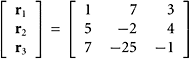
SOLUTION Yes. We observe that −3r1 + 2r2 − r3 = 0, where ri is the ith row in the matrix.
EXAMPLE 8
Consider the three polynomials defined as follows: p1(t) = 7t5 − 4t2 + 3, p2(t) = 2t5 + 5t2, p3(t) = 8t5 − 23t2 + 6. Is the set {p1, p2, p3} linearly independent?
SOLUTION No. We notice that 2p1 − 3p2 − p3 = 0.
SOLUTION The answer is no, because C = 3A − B.
EXAMPLE 10
Let  ,
,  ,
, 
Is {u1, u2, u3} linearly independent? What about {u1, u2}?
SOLUTION For the first set, we consider the equation c1u1 + c2u2 + c3u3 = 0. The issue is whether this equation has a nontrivial solution. The coefficient matrix for the problem is
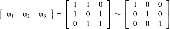 |
|
Here we do not include the righthand side because the system of equations is homogeneous and the righthand side consists of zeros. Hence, we obtain c1 = c2 = c3 = 0, and the set is linearly independent. For the second set, we look at just the first two columns in the preceding matrix. Of course, the conclusion is the same.
EXAMPLE 11
Let ![]() ,
, ![]() ,
, ![]()
Is the set {A, B, C} linearly independent?
SOLUTION How can we identify these 2 × 2 matrices with column vectors so that we can treat them in the same manner as in Example 10? We make them into vectors, which exactly correspond to each matrix:
 |
|
Because the only solution is [0, 0, 0]T, the given set of matrices is linearly independent.
Later, in Section 5.2, we shall justify fully the method used in Example 11. It hinges on the fact that ![]() is isomorphic to
is isomorphic to ![]() .
.
DEFINITION
Consider a finite, indexed set of vectors {u1, u2, …, um} in a vector space. We say that the indexed set is linearly dependent if there exist scalars ci such that
|
If the indexed set is not linearly dependent, we say that it is linearly independent. The expression ![]() implies that at least one ci is nonzero.
implies that at least one ci is nonzero.

SOLUTION Label the rows of A as r1, r2, and r3. This is understood to be an indexed set. (Each vector has an index attached to it.) In the definition of linear dependence, we can take c1 = 1, c2 = 0, and c3 = −1 because r1 − r3 = 0. The indexed set of rows contains three rows with the vector (2, 5, 7) appearing twice. If we are interested only in the set, we need not mention this vector twice. Thus, the set consists of two vectors, (2, 5, 7) and (4, 1, −5). There is a difference between the set and the indexed set. In this example, the latter is linearly dependent, whereas the former is linearly independent. In an indexed set, we consider the vector u1 =(2, 5, 7) to be different from u3 = (2, 5, 7) because their indices (1 and 3) are different.
In an effort to avoid confusion we always consider the rows (or the columns) of a matrix to be indexed sets.

SOLUTION It is linearly independent, because when we try to solve the equation Ax = 0 for x, we discover that x = 0 is the only solution.
EXAMPLE 14
How can we test to determine whether the rows of the matrix in Example 13 form a linearly independent set?
SOLUTION Apply the technique of Example 13 to the transposed matrix
 |
|
The equation ATx = 0 has only the trivial solution (x = 0), and the set in question is linearly independent. Later we will prove theorems that make such questions easier to answer.
THEOREM 6
Each vector in the span of a linearly independent set (in a vector space) has a unique representation as a linear combination of elements of that set.
PROOF Let x be a point in the span of S, where we suppose S to be a linearly independent set. Then ![]() , for appropriate ai ∈
, for appropriate ai ∈ ![]() and ui ∈ S. Suppose there is another such representation,
and ui ∈ S. Suppose there is another such representation, ![]() , where bi ∈
, where bi ∈ ![]() and vi ∈ S. Put U = {u1, u2, …, un} and V = {v1, v2, …, vm}. Consider
and vi ∈ S. Put U = {u1, u2, …, un} and V = {v1, v2, …, vm}. Consider
|
(Here, k is not necessarily n + m.) All the points wi are different from each other and belong to S. Because S is linearly independent, so is U ∪ V. By supplying zero coefficients, if necessary, we can write ![]() and
and ![]() . By subtraction, we get
. By subtraction, we get ![]() . Because U ∪ V is linearly independent, all the coefficients in this last equation are zero. Hence, we obtain ci = di for all i.
. Because U ∪ V is linearly independent, all the coefficients in this last equation are zero. Hence, we obtain ci = di for all i.
EXAMPLE 15
In two different ways, express the vector [5, 3, 5]T in terms of the three columns in the matrix of Example 12.
SOLUTION If we take a linear combination of these columns with coefficients (−3, 5, −2), we get the same vector as when we use coefficients (13, −14, 7). (In both cases the result is the vector [5, 3, 5]T.) By Theorem 6, the columns in question must form a linearly dependent set.
THEOREM 7
If a matrix has more columns than rows, then the (indexed) set of its columns is linearly dependent.
PROOF Let A be m × n, and n > m. Think of what happens if we try to solve the equation Ax = 0. This is a homogeneous equation with more variables (n) than equations (m). By Corollary 2 in Section 1.3, such a system must have nontrivial solutions.
EXAMPLE 16
Let  ,
, 
 ,
, 
Is the set{v1, v2, v3, v4} linearly independent?
SOLUTION Put the vectors into a matrix as columns. The resulting matrix will have three rows and four columns:
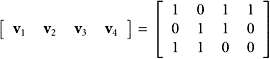 |
|
By Theorem 7, the set of columns is linearly dependent.
THEOREM 8
Any (indexed) set of more than n vectors in ![]() is necessarily linearly dependent.
is necessarily linearly dependent.
PROOF Put the vectors as columns into an n × m matrix, and apply Theorem 7.
THEOREM 9
Let {u1, u2, …, um} be a linearly dependent indexed set of at least two vectors (in a vector space). Then some vector in the indexed list is a linear combination of preceding vectors in that list.
PROOF By hypothesis, there is a relation ![]() , in which the coefficients ci are not all 0. Let r be the last index for which cr ≠ 0. Then ci = 0 for i > r and
, in which the coefficients ci are not all 0. Let r be the last index for which cr ≠ 0. Then ci = 0 for i > r and ![]() . Because cr ≠ 0, this last equation can be solved for ur, showing that ur is a linear combination of the preceding vectors in the set.
. Because cr ≠ 0, this last equation can be solved for ur, showing that ur is a linear combination of the preceding vectors in the set.
THEOREM 10
If a vector space is spanned by some set of n vectors, then every set of more than n vectors in that space must be linearly dependent.
PROOF Let {v1, v2, …, vn} span a vector space V, and let {u1, u2, …, um} be any subset of V such that m > n. By the definition of span, there exist coefficients aij such that ![]() for 1 ≤ i ≤ m. Consider the homogeneous system of equations
for 1 ≤ i ≤ m. Consider the homogeneous system of equations ![]() . This system has fewer equations than unknowns. Therefore, Corollary 2 in Section 1.3 is applicable, and there must exist a nontrivial solution, x = (x1, x2, ···, xm). Now we see that the set of vectors ui is linearly dependent, because
. This system has fewer equations than unknowns. Therefore, Corollary 2 in Section 1.3 is applicable, and there must exist a nontrivial solution, x = (x1, x2, ···, xm). Now we see that the set of vectors ui is linearly dependent, because
|
THEOREM 11
Let S be a linearly independent set in a vector space V. If x ∈ V and x ∈ Span(S), then S ∪ {x} is linearly independent.
PROOF If that conclusion is false, there must exist a nontrivial equation of the form ![]() where the points vi belong to S and the ci are scalars, not all zero. If c0 = 0, then that equation will contradict the linear independence of the set S. Hence, we obtain c0 ≠ 0 and
where the points vi belong to S and the ci are scalars, not all zero. If c0 = 0, then that equation will contradict the linear independence of the set S. Hence, we obtain c0 ≠ 0 and ![]() , showing that x is in the span of S.
, showing that x is in the span of S.
EXAMPLE 17
Here is an example involving an infinite set of vectors. Let pj(t) = tj for j = 0, 1, 2, 3, …. These functions are called monomials and they are the building blocks of all polynomials. They also lie in the vector space of all continuous functions ![]() →
→ ![]() . Is the set {pj : j = 0, 1, 2, …} linearly independent?
. Is the set {pj : j = 0, 1, 2, …} linearly independent?
SOLUTION The answer is yes and deserves a proof. We shall use the method of contradiction to carry out this proof. Suppose therefore that the set of functions pj is linearly dependent. (Then we hope to arrive at a contradiction.) From the definition of linear dependence, there must exist a nontrivial equation of the form
|
(In this context, nontrivial means that the coefficients cj are not all zero.) Think about this displayed equation. Does it not say that a certain nontrivial polynomial of degree at most m is, in fact, equal everywhere to 0? One need only recall from the study of algebra that a nontrivial polynomial of degree k can have at most k zeros (or roots). See Appendix B, Theorem B.1. We have reached a contradiction.
Observe that linear dependence always involves a linear combination of vectors, and a linear combination is always restricted to a finite set of terms. We cannot consider infinite series of vectors without bringing convergence questions into play, and that is another story altogether.
Linear Mapping
The concept of a linear mapping was introduced in Section 2.3. It is meaningful for maps between any two vector spaces. The characteristic property is T(ax + by) = aT(x) + bT(y). Let us illustrate this matter with a linear space of polynomials.
Consider the space ![]() , consisting of all polynomials whose degree does not exceed 3. (This is an important example of a vector space.) We can use the following natural basic polynomials for this space: pj(t) = tj, where 0 ≤ j ≤ 3. Thus, we have p0(t) = 1, p1(t) = t, p2(t) = t2, and p3(t) = t3. Every element of
, consisting of all polynomials whose degree does not exceed 3. (This is an important example of a vector space.) We can use the following natural basic polynomials for this space: pj(t) = tj, where 0 ≤ j ≤ 3. Thus, we have p0(t) = 1, p1(t) = t, p2(t) = t2, and p3(t) = t3. Every element of ![]() is a unique linear combination of these four basic polynomials. For example, the polynomial f defined by f(t) = 7 − 3t + 9t2 − 5t3 is expressible as f = 7p0 − 3p1 + 9p2 − 5p3. Consequently, if g is a polynomial of degree at most 3, and if
is a unique linear combination of these four basic polynomials. For example, the polynomial f defined by f(t) = 7 − 3t + 9t2 − 5t3 is expressible as f = 7p0 − 3p1 + 9p2 − 5p3. Consequently, if g is a polynomial of degree at most 3, and if ![]() , then we can represent g by the vector (c0, c1, c2, c3). If T is a linear transformation from
, then we can represent g by the vector (c0, c1, c2, c3). If T is a linear transformation from ![]() into some other vector space, we will have
into some other vector space, we will have
|
This easy calculation shows that a linear map is completely determined as soon as its values have been prescribed on a set that spans the domain.
Caution: The values assigned are not necessarily unrestricted.
EXAMPLE 18
For a concrete case of the preceding idea, suppose that T maps ![]() into
into ![]() according to the following rules:
according to the following rules:
|
What is the matrix for this transformation?
SOLUTION For u = c0p0 + c1p1 + c2p2 + c3p3, we have
 |
|
EXAMPLE 19
Use the information in Example 18 to find the effect of applying T to the polynomial u(t) = 4t3 − 2t2 + 3t − 5.
SOLUTION We note that the representation of this polynomial by a vector in ![]() is (−5, 3, −2, 4). (One must write the terms in the correct order.) The answer to the question is therefore
is (−5, 3, −2, 4). (One must write the terms in the correct order.) The answer to the question is therefore
 |
|
A theorem to formalize what we have seen in the preceding examples is as follows.
THEOREM 12
Let {u1, u 2, … un} be a linearly independent set in some vector space. Let v1, v2, …, vn be arbitrary vectors in another vector space. Then there is a linear transformation T such that T(ui) = vi for 1 ≤ i ≤ n.
PROOF The linear transformation will be defined on the set U = Span{u1, u2, … un} by this equation:
|
We must recall that any vector in U has one and only one representation as a linear combination of the vectors ui.
EXAMPLE 20
Is there a linear transformation that maps (1, 0) to (5, 3, 4) and maps (3, 0) to (1, 3, 2)?
SOLUTION Let T be such a map. Being linear, T must obey the equation T(cx) = cT(x). Hence, we have
|
The answer to the question posed is no.
Theorem 12 does not apply in Example 20 because the pair of vectors (1, 0) and (3, 0) is not linearly independent. A slightly different point of view is that (3, 0) − 3(1, 0) = 0 and therefore by linearity we must have T(3, 0) − 3T(1, 0) = 0. This leads to the following theorem.
THEOREM 13
If T is a linear transformation, then any linear dependence of the type ![]() must imply
must imply ![]() .
.
Consequently, if {ui} is linearly dependent, then {T(ui)} is linearly dependent, and if {T(ui)} is linearly independent, then {ui} is linearly independent.
Application: Models in Economic Theory
Linear algebra has a large role to play in economic theory. Two simple, yet basic, economic models are discussed here.
Think of a nation’s economy as being divided into n sectors, or industries. For example, we could have the steel industry, the shoe industry, the medical industry, and so on. (In a realistic model, there could be 1000 or more sectors.) An n × n matrix A = (aij) is given; it contains data concerning the productivity of the n sectors. Specifically, aij is the fraction of the output from industry j that goes to industry i as input in one year. We assume in a closed model that all the output of the various industries remains in the system and is purchased by the sectors in the system. Because of this assumption (that the system is closed), the column sums in the matrix A are 1:
|
Let xj be the value placed on the output from the jth sector in one year. The price vector x = (x1, x2, …, xn) is unknown but will be determined after certain requirements have been imposed on it.
An equilibrium state occurs if the price vector x is a nonzero vector x = (x1, x2, …, xn) such that Ax = x. Notice that if x has this property, then any nonzero scalar multiple of x will also have that property.
THEOREM 14
If A is a square matrix whose column sums are all equal to 1, then the equation Ax = x has nontrivial solutions.
PROOF The equation in question is (I − A)x = 0. The coefficient matrix here is singular (noninvertible) because its rows add up to 0. Consequently, the kernel of I − A contains nonzero vectors.
This model is called the Leontief Closed Model in honor of Wassily Leontief.5 The model described is said to be closed because the sectors in the model satisfy the needs of all sectors, but no goods leave or enter the system.
5 Professor Wassily Leontief (1906–1999) was awarded the 1973 Nobel Prize in Economics for his work on mathematical models in economic theory. Leontief was born in St. Petersburg, Russia. He was arrested several times for criticizing the control of intellectual and personal freedom under communism. In 1925, he was allowed to leave the country because the authorities believed that he had a cancerous growth on his neck that would soon kill him. The growth turned out to be benign, and Leontief earned a Ph.D. in Berlin prior to his immigration to the United States in 1931. He served as a professor at Harvard University and later at New York University. He began compiling the data for the input–output model of the United States economy in 1932, and in 1941 his paper Structure of the American Economy, 1919–1929 was published. Leontief was an early user of computers, beginning in 1935 with large-scale mechanical computing machines and, in 1943, moving on to the Mark I, the first large-scale electronic computer.
All of the elements of the matrix A are nonnegative, and the elements in each column sum to 1. The matrix A occurring here is called an input– output matrix or consumption matrix. If x is a solution of the equation, then scalar multiples of x will also be solutions. The equation Ax = x indicates that x is a fixed point of the mapping x ![]() Ax. Solving the equation (I − A)x = 0 is easily done: we are looking for a nontrivial solution to a system of homogeneous equations.
Ax. Solving the equation (I − A)x = 0 is easily done: we are looking for a nontrivial solution to a system of homogeneous equations.
To illustrate the Leontief Closed Model, we consider an example involving three sectors S1, S2, and S3. The pertinent information is given in this table:
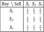
The entries in the table form the matrix A. Notice that the column sums are all 1. The consumption matrix, I − A, is shown here along with its reduced echelon form:
 |
|
The general solution of this homogeneous system is x1 = x3 and ![]() , where x3 is a free variable. One simple solution is x = (4, 3, 4). (All solutions are multiples of this one.) The rows in the input–output table above show how the three commodities go from source to user (seller to buyer) in the economy. The flow of commodities between the different sectors can be shown in a graph as in Figure 2.27. Row 1 of the table indicates that for sector S1 to produce one unit of its product it must consume one-fourth of its own product, one-third of sector S2’s product, and one-half of sector S3’s product. There are similar flows in the other sectors.
, where x3 is a free variable. One simple solution is x = (4, 3, 4). (All solutions are multiples of this one.) The rows in the input–output table above show how the three commodities go from source to user (seller to buyer) in the economy. The flow of commodities between the different sectors can be shown in a graph as in Figure 2.27. Row 1 of the table indicates that for sector S1 to produce one unit of its product it must consume one-fourth of its own product, one-third of sector S2’s product, and one-half of sector S3’s product. There are similar flows in the other sectors.
Usually, an economy has to satisfy some outside demands from non-producing sectors such as government agencies. In this case, there is also a final demand vector b = (bi), which lists the demands placed upon the various industries for output unconnected with the industries mentioned previously. With xi and cij as previously defined, we are led to the equations: ai1x1 + ai2x2 + ··· + ainxn + bi = xi. The linear system for the Leontief Open Model is
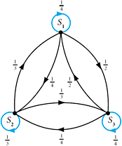
FIGURE 2.27 Flow among three sectors.
|
The term Ax is called the intermediate demand vector and b is the final demand vector. In this case, the elements of the matrix A are nonnegative and the column sums are less than 1.
To illustrate the Leontief Open Model, we consider a simple example involving two industrial sectors S1 and S2 as given by this table:
Suppose that the initial demand vector is b = (350, 1700). Then we solve the system
|
and obtain the solution x = (1000, 2000). The flow between the different sectors in this input–output table can be illustrated by the graph shown in Figure 2.28.

FIGURE 2.28 Flow example between two sectors.
A common question in input–output analysis is: Given a forecasted demand, how much output from each of the sectors would be needed to satisfy the final demand? If we increase the final demand to $400 for sector S1 and decrease it to $1600 for sector S2, we have the new demand vector b = (400, 1600). Here the change in final demand is Δb = (50, −100). Solving the system
|
we find Δx = (29.70, −99.01), which is the change in the output vector. This change in demand requires an increase in production by sector S1 and a decrease in S2. Consequently, the new output vector is x ≈ (1030, 1900). This process can be repeated for different possible situations.
In Section 8.3, the Leontief models are studied in greater detail.
SUMMARY 2.4
• A vector space is a set V of vectors, together with vector addition and scalar multiplication that satisfy the following axioms:
• If u, v ∈ V, then u + v ∈ V.
(Closure axiom for addition)
• For all u, v ∈ V, u + v = v + u.
(Commutativity of vector addition)
• For any u, v, w ∈ V, (u + v) + w = u + (v + w).
(Associativity of vector addition)
• There is a zero element 0 ∈ V such that u + 0 = u, for all u ∈ V.
(Existence of a zero vector)
• For each vector u ∈ V there is at least one element ![]() ∈ V such that
∈ V such that ![]() + u = 0.
+ u = 0.
(Existence of additive inverses)
• If u ∈ V and α ∈ ![]() , then αu ∈ V.
, then αu ∈ V.
(Closure axiom for scalar–vector product)
• For any α ∈ ![]() and u, v ∈ V, α(u + v) = αu + αv. (Distributive law: scalar times vectors)
and u, v ∈ V, α(u + v) = αu + αv. (Distributive law: scalar times vectors)
• If α, β ∈ ![]() and u ∈ V, then (α + β)u = αu + βu. (Distributive law: scalar sum times a vector)
and u ∈ V, then (α + β)u = αu + βu. (Distributive law: scalar sum times a vector)
• If α, β ∈ ![]() and u ∈ V, then α(βu) = (αβ)u. (Associativity of scalar–vector product)
and u ∈ V, then α(βu) = (αβ)u. (Associativity of scalar–vector product)
• For each u ∈ V, 1 · u = u. (Multiplication of unit scalar times vector)
• In any vector space, if c ∈ ![]() , then c0 = 0.
, then c0 = 0.
• In a vector space V, if x ∈ V, c ∈ ![]() , and cx = 0, then either c = 0 or x = 0.
, and cx = 0, then either c = 0 or x = 0.
• In a vector space, for each x ∈ V, the point ![]() is uniquely determined. (Recall that x +
is uniquely determined. (Recall that x + ![]() = 0.)
= 0.)
• In a vector space, every vector x ∈ V satisfies the equation 0x = 0.
• In any vector space, for each x ∈ V, we have (−1)x = ![]() .
.
• A subset S in a vector space is linearly dependent if there exists a nontrivial equation of the form c1u1 + c2u2 + ··· + cmum = 0, where the distinct points u1, u2, …, um come from S.
• Each vector in the span of a linearly independent set (in a vector space) has a unique representation as a linear combination of elements of that set.
• If a matrix has more columns than rows, then the indexed set of its columns is linearly dependent.
• Any indexed set of more than n vectors in ![]() is necessarily linearly dependent.
is necessarily linearly dependent.
• Let {u1, u2, …, um} be a linearly dependent indexed set of at least two vectors (in a vector space). Then some vector in the indexed list is a linear combination of preceding vectors in that list.
• If a matrix has more columns than rows, then the indexed set of its columns is linearly dependent.
• If a vector space is spanned by some set of n vectors, then every set of more than n vectors in that space must be linearly dependent.
• Let S be a linearly independent set in a vector space V. If x ∈ V and x ∉ Span(S), then S ∪ {x} is linearly independent.
• Let {u1, u2, … un} be a linearly independent set in some vector space. Let v1, v2, …, vn be arbitrary vectors in another vector space. Then there is a linear transformation T such that T(ui) = vi for 1 ≤ i ≤ n.
• If T is a linear transformation, then any linear dependence of the type ![]() must imply
must imply ![]() .
.
• If A is a square matrix whose column sums are all 1, then the equation Ax = x has nontrivial solutions.
• Leontief Closed Model: (I − A)x = 0; Leontief Open Model: (I − A)x = b.
KEY CONCEPTS 2.4
Vector spaces, axioms for vector spaces, spaces of sequences, spaces of functions, spaces of polynomials, linear independence, linear dependence, spaces of matrices, vector subspaces, indexed set, Leontief Closed Model
GENERAL EXERCISES 2.4
1. Determine whether this set of four vectors is linearly dependent or linearly independent: {(1, 3, 2, −1), (4, −1, 5, 1), (−2, 1, 1, 7), (12, 2, 6, −22)}
2. Consider the set {p1, p2, p3, p4}. Determine whether this set of polynomials is linearly independent or linearly dependent. The definitions are p1(t) = 1, p2(t) = t, p3(t) = 4 − t, p4(t) = t3.
3. Let f(t) = sin t and g(t) = cos t. Determine whether the pair {f, g} is linearly dependent or linearly independent.
4. Let f(t) = 1, g(t) = cos 2t, and h(t) = sin2 t. Determine whether the set {f, g, h} is linearly dependent or independent.
5. Test each of these sets of functions for linear dependence or linear independence:
a. u1(t) = 1, u2(t) = sin t, u3(t) = cos t
b. w1(t) = 1, w2(t) = sin2 t, w3(t) = cos2 t
c. v1(t) = cos 2t, v2(t) = sin2 t, v3(t) = cos2 t
6. Define polynomials p0(t) = t + t2 + t3, p1(t) = t3 + t4 + t5, p2(t) = t5 + t6 + t7. Verify the assertion or find a counterexample: {p0, p1, p2} is linearly dependent.
7. Consider the matrix 
Do its rows form a linearly dependent set?
8. Consider ![]() ,
, ![]() ,
, ![]()
Is this set of three matrices linearly independent?
9. Let u = (7, 1, 2), v = (3, −2, 4), and w = (6, 13, −14). Find a simple description of Span {u, v} ∩ Span{w} and Span{u, v} + Span{w}.
10. Let {x, y, z} be a linearly independent set of three vectors in some vector space. Justify the assertion or find a counterexample: {2x + 3y − z, 4y + 2z, 3z} is linearly independent.
11. Is the following example a vector space?
![]()
12. Consider any set of four vectors in ![]() . It must be linearly dependent. Why?
. It must be linearly dependent. Why?
13. Let ![]() be as given. In each case, find the kernel of L.
be as given. In each case, find the kernel of L.
a. (Lp)(t) = 2p′(t) + 3tp″(t)
b. Lp = 2p′ + 3p″
14. Define three polynomials as follows: p1(t) = t3 + t, p2(t) = t2 + 1, and p3(t) = 3t3 − 2t2 + 3t − 2.
Is the set {p1, p2, p3} linearly independent?
15. Define these polynomials: p1(t) = 1 + t2, p2(t) = 2t − 4, p3(t) = 1 + t + t2.
Does {p1, p2, p3} span ![]() ?
?
16. Consider p0(t) = 1, p1(t) = 1 + t, p2(t) = 1 + t + t2. Give an argument why Span {p0, p1, p2} = ![]() , the set of all polynomials of degree less than or equal to 2.
, the set of all polynomials of degree less than or equal to 2.
17. Does the set of all vectors in ![]() that have exactly two zero entries span
that have exactly two zero entries span ![]() ?
?
18. Let v1 = [1, 0, 0, 0]T, v2 = [0, 1, 0, 0]T, and v3 = [0, 0, 1, 0]T. Is the set of these three vectors linearly independent? Why?
19. Justify each step in this alternative proof of Theorem 1: 0 = 0 + 0, c0 = c0 + c0, c0 − c0 = c0, 0 = c0.
(Use only the axioms of a vector space.)
20. Define the standard monomial functions: p0(t) = 1, p1(t) = t, p2(t) = t2, and soon. Is this set linearly independent if we take the domain of these functions to be the set of all positive integers?
21. Discuss the question of whether the set of all discontinuous functions defined on [−1, 1] forms a vector space. (Refer to Example 2.)
22. Verify that if {v1, v2, v3} is linearly independent, then so is the set {v3 + v2, v1 + v3, v2 + v1}.
23. Establish that a set of two vectors is linearly dependent if and only if one of the vectors is a multiple of the other.
24. Consider a sequence of polynomials pk, where k = 0, 1, 2, …. Assume that for all k, the polynomial pk has degree k. Thus, the highest power present in pk is tk, and it occurs with a nonzero coefficient. Explain why the set {pk : k = 0, 1, 2, …} is linearly independent. Suggestion: Begin with a simple case: {p0, p1, p2}.
25. Establish that if a set of two or more nonzero vectors is linearly dependent, then one element of the set is a linear combination of the others.
26. Let {u1, u2, …, un} be a linearly independent set in a vector space. Explain that if ![]() , then (α1, α2, …, αn) = (β1, β2, …, βn).
, then (α1, α2, …, αn) = (β1, β2, …, βn).
27. Let G and H be subsets of a vector space, and suppose that G ⊆ H. (Thus, G is a subset of H: each element of G is in H.) Establish the following:
a. If H is linearly independent, then so is G.
b. If G spans the vector space, then so does H.
c. In some cases, G can be linearly independent while H is not.
d. In some cases, H can span the vector space while G does not.
28. In the axioms for a vector space, can Axioms 2 and 3 be replaced by a single axiom that states (u + v) + w = v + (u + w)?
29. Establish that if {u1, u2, ···, um} is a linearly independent set in Span{v1, v2, …, vn}, then m ≤ n.
30. In the axioms for a vector space, can we dispense with the fifth one, and still prove that u + (−1)u = 0?
31. Let V be the set of all positive real numbers. In V, define ![]() and
and ![]() for α ∈
for α ∈ ![]() , u ∈ V, v ∈ V. Establish that V, with the operations just defined, is a vector space. (This example is found in many texts, such as that of Andrilli and Hecker, [1998] and Ikramov [1975]. We call it an exotic vector space, since it is so different from the familiar examples. See also the next exercise.)
, u ∈ V, v ∈ V. Establish that V, with the operations just defined, is a vector space. (This example is found in many texts, such as that of Andrilli and Hecker, [1998] and Ikramov [1975]. We call it an exotic vector space, since it is so different from the familiar examples. See also the next exercise.)
32. This is another exotic vector space, similar to one in the textbook of Andrilli and Hecker [1998]. Verify all the axioms for a vector space. Let V be the set ![]() with new definitions of vector addition and multiplication of scalars: (x1, x2)
with new definitions of vector addition and multiplication of scalars: (x1, x2) ![]() (y1, y2) = (x1 + y1 + a, x2 + y2 + b) and λ
(y1, y2) = (x1 + y1 + a, x2 + y2 + b) and λ ![]() (x1, x2) = (λx1 + λa − a, λx2 + λb − b). Here, a and b are arbitrary constants, fixed at the outside.
(x1, x2) = (λx1 + λa − a, λx2 + λb − b). Here, a and b are arbitrary constants, fixed at the outside.
33. Establish that if V is a vector space, then ![]() is a vector space with the standard definitions of the two algebraic operations. The notation YX denotes the set of all functions from X to Y.
is a vector space with the standard definitions of the two algebraic operations. The notation YX denotes the set of all functions from X to Y.
34. Is Span(S) + Span(T) = Span(S ∪ T) true for subsets S and T in a vector space? A proof or counterexample is required. See Section 1.2, for the definition of the span of a set. The sum of two sets, U and V, is the set {u + v : u ∈ U, v ∈ V}. This is not the same as their union.
35. The symbol ![]() denotes the set of all complex numbers, x + iy, where i2 = −1, and x and y are real. The notation
denotes the set of all complex numbers, x + iy, where i2 = −1, and x and y are real. The notation ![]() denotes a space like
denotes a space like ![]() except that we allow the vectors to have complex components. Verify that
except that we allow the vectors to have complex components. Verify that ![]() together with
together with ![]() as the field of scalars is a vector space. (See Appendix B.)
as the field of scalars is a vector space. (See Appendix B.)
36. Explain this: If S is a linearly dependent set, then there is an element v in S such that the span of S is the same as the span of S{v}. If there are two such elements in S, can we remove both without changing the span? (Here ST = {x : x ∈ S and x ∉ T}.)
37. Establish that in a vector space the zero element is unique.
38. Let S be a linearly independent set in a vector space V. Let x be a point in V that is not in Span(S). Explain why the set S ∪ {x} is linearly independent.
39. Let {x, y, z} be a linearly independent set of three vectors in some vector space. Explain the assertion or find a counterexample: {x + y + z, x + y, x} is linearly independent.
40. Consider a finite set of polynomials, not containing the 0-polynomial, and having the property that any two polynomials in the set will have different degrees. Establish that the set is linearly independent. (In case of difficulty, look at small examples.) Perhaps you can improve on this theorem.
41. Let X and Y be two sets of vectors in some linear space. Assume that each x in X is in the span of Y, and each y in Y is in the span of X. Explain why X and Y have the same span.
42. Define what is meant by saying that a set in a vector space is linearly dependent.
43. Let S and T be subsets of a vector space, and assume that S ⊆ T. (This means that S is a subset of T: each member of S is a member of T.) Establish that Span(S) ⊆ Span(T).
44. A function f : ![]() →
→ ![]() is continuous at a point x0 if for any ε > 0 there corresponds a δ > 0 such that |x − x0| < δ implies |f(x) − f(x0)| < ε. Explain why the hypothesis f and g are continuous at x0 leads to f + g being continuous at x0.
is continuous at a point x0 if for any ε > 0 there corresponds a δ > 0 such that |x − x0| < δ implies |f(x) − f(x0)| < ε. Explain why the hypothesis f and g are continuous at x0 leads to f + g being continuous at x0.
45. Verify that the set of all 2 × 2 matrices under the usual operations is a vector space.
46. Explain these: if A is m × n and m > n (more rows than columns), then the rows of A form a linearly dependent set. Equivalently, if B is m × n and n > m (more columns than rows), then the columns of B form a linearly dependent set.
47. If n < m, is ![]() a subspace of
a subspace of ![]() ? Under what conditions is
? Under what conditions is ![]() a subspace of
a subspace of ![]() ? (
? (![]() is the vector space of all polynomials whose degrees are at most n.)
is the vector space of all polynomials whose degrees are at most n.)
48. Let {u1, u2, …, un} be a linearly independent set in a vector space. Establish that if ![]() , then (α1, α2, …, αn) = (β1, β2, …, βn).
, then (α1, α2, …, αn) = (β1, β2, …, βn).
49. If S is a set (without any algebraic structure) and if V is a vector space, is VS avector space? Explain. (The notation VS denotes the set of all mappings from S to V.)
50. (Continuation.) With the hypotheses of the preceding problem, is SV a vector space? Explain.
51. Are these vector spaces?
a. The vectors are in ![]() and the scalars can be in
and the scalars can be in ![]() .
.
b. The vectors are members of ![]() , but the scalars are confined to be in
, but the scalars are confined to be in ![]() . (See Appendix B on complex arithmetic.)
. (See Appendix B on complex arithmetic.)
52. Explain and write out in detail the following.
a. Example 1.(Verify all of the vector-space axioms.)
b. Why is a subspace more than a subset?
c. Example 13.
d. Example 14.
COMPUTER EXERCISES 2.4
1. Use mathematical software to solve this Leontief system involving
 |
|
2. Suppose that an economy consists of four sectors, labeled Sa, Sb, Sc, and Sd. The interactions between the sectors are governed by a table as follows:

Solve the corresponding system when the final demand vector is b = (25, 10, 30, 45).
3. Let 
Using a mathematical software system, solve the Leontief Open Model with the following data for the different final demand vectors: (6, 9, 8), (9, 12, 16), (12, 18, 32).
4. By generating a large number of two component random integer vectors, determine experimentally the percentage of times they are linearly independent and linearly dependent.
5. (Continuation.) Repeat with three component random integer vectors.