CHAPTER FOUR
Determinants
4.1 DETERMINANTS: INTRODUCTION
I was x years old in the year x2.
—AUGUSTUS DE MORGAN (1806–1871), RESPONDING TO THE QUESTION OF HOW OLD HE WAS
To speak algebraically, Mr. M. is execrable, but Mr. C. is x plus 1 - ecrable.
—EDGAR ALLAN POE (1809–1849)
Properties of Determinants
With every square matrix there is associated a real number called the determinant of that matrix. The notation used here is Det(A) or Det A for the determinant of A. There are various ways to present postulates for determinants from which all other properties follow. We have chosen to start with the following three basic properties of determinants because they lead directly to their efficient calculation.
PROPERTIES OF DETERMINANTS
I. The determinant of a triangular matrix is the product of its diagonal elements. (triangular matrix)
II. If a matrix à results from a matrix A by adding a multiple of one row onto another row, then Det(Ã) = Det(A). (replacement)
III. If the matrix à results from a matrix A by multiplying one row of A by a constant c, then Det(Ã) = c Det(A). (scaling)
It is not clear that such a function Det exists and is unambiguous. In other words, at this stage we do not know whether a determinant function exists or whether it is unique. We shall proceed nevertheless and use the fact that the three Properties I, II, and III can be used to arrive at a unique value for the determinant of any (square) matrix. Historically, determinants preceded matrices by more than 150 years, and many facts in matrix theory were originally discovered and developed from determinant theory. See Thomas Muir [1960] for the historical development of determinants from the time of Leibniz to 1920.
EXAMPLE 1
We can already compute the determinants of some matrices with almost no effort. Test your understanding of the Properties I, II, and III, by evaluating the determinants of these four matrices.
 |
|
SOLUTION The first matrix is upper triangular, and, by Property I, its determinant is (4)(3)(10) = 120. In the second matrix, we can add −2 times row 1 to row 2 without changing the determinant. This brings us to the matrix  . The determinant of this upper triangular matrix is (3)(7)(5) = 105. The third matrix, being nonsquare, has no determinant. (The determinant function is defined only for square matrices.) The fourth matrix is lower triangular, and, by Property I, its determinant is 24.
The list of Properties I, II, and III is almost a minimal set of assumptions: they do allow the whole theory of determinants to be deduced from them. In a complete development of the subject, we would prove that there exists one and only one such function, Det. The assumptions postulated in Properties I, II, and III are stronger than those given in the pioneering textbook of Stoll [1952]. For example, Stoll assumes (instead of Property I) that the determinant of every identity matrix is 1. The later revision of this book, Stoll and Wang [1968], is another source for this theory. The books by Strang [1988, 2003] have lucid accounts of this topic based on a different set of postulates: Det(A) depends linearly on row 1, Det(A) changes sign when two rows are swapped, and Det(I) = 1.
First we draw an easy but useful conclusion from the Properties I, II, and III. The property in the following theorem is not an assumption but rather a consequence of the Properties I, II, and III.
PROOF Recall from Section 1.1, that a swap (or interchange) of two rows is accomplished by this sequence of the two other types of row operations:
|
The first three row operations have no effect on the determinant, by Property II. The fourth row operation changes the sign of the determinant, by Property III. Hence, the total effect is to change the sign of the determinant when two rows are interchanged.
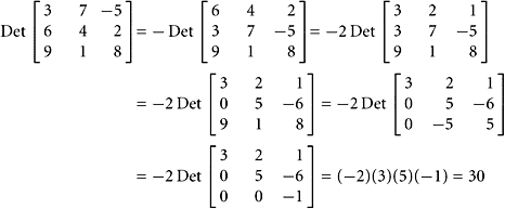
SOLUTION The first equation is true by Theorem 1. The next is justified by Property III. The next three equalities follow from Property II. The last equality uses Property I.
We can compute many determinants with only Properties I and II. The purpose of the Properties II and III, and Theorem 1 is to keep track of the effect on a determinant when row operations are used to arrive at a triangular form.
Example 2, and the working out of the determinant therein, raises the question hinted at earlier: ‘‘How can we be sure that no matter what sequence of row operations we use to compute the determinant, the result will be the same?’’ Eventually, it is necessary to establish the existence and uniqueness of a determinant function that has the properties expressed in the three Properties I, II, and III.
THEOREM 2
There is one and only one determinant function having Properties I, II, and III.
Theorem 2 is stated without proof. It is needed to justify the algorithm for computing determinants.
An Algorithm for Computing Determinants
We are now in a position to calculate the determinant of any square matrix, by using Properties I, II, and III and Theorem 1. The idea is very simple: Given a (square) matrix, A, use the Properties I, II, and III, as well as Theorem 1 to find a triangular matrix A that is row equivalent to A. Along the way, keep track of any changes in the determinant caused by the use of Property III and Theorem 1. At the end, apply Property I. The deeper truth, which we are not going to prove, is that a unique value arises, despite the fact that different sequences of row operations may have been used.

SOLUTION Here are the steps, using Property II repeatedly and finally Property I:
 |
|
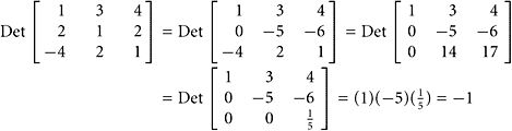
EXAMPLE 4
Using the matrix in Example 3, compute its determinant, but with a different sequence of operations. Start by using Theorem 1.
SOLUTION
 |
|
In theory, we could establish formulas for determinants of arbitrary square matrices having any size: 1 × 1, 2 × 2, 3 × 3, and so on. The formulas quickly become unmanageable, however. If a matrix is 1 × 1, then it is triangular, and Det[a] = a by Property I. The next case is the general 2 × 2 matrix. To get a formula for its determinant, let ![]() . If c = 0, then the matrix is already upper triangular, and Det (A) = ad = ad − bc. If c ≠ 0, then we get the same result by first performing a row swap followed by another row operation:
. If c = 0, then the matrix is already upper triangular, and Det (A) = ad = ad − bc. If c ≠ 0, then we get the same result by first performing a row swap followed by another row operation:
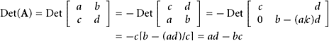 |
|
Thus, in both cases, we get ad − bc. This formula is worth remembering, since in many calculations involving determinants the 2 × 2 case is needed.

SOLUTION One way to do it is shown here:
 |
|
Here we have performed two swaps and some extra steps to avoid fractions.
Algorithm without Scaling
Here is a slightly different algorithm for computing the determinant of any square matrix A. Use the row-reduction process without scaling and keep track of the number of row interchanges. To reduce A to upper triangular form, Ã, we use Properties I and II and Theorem 1, but not Property III. Let k be the number of row swaps employed in this process. Then the determinant of the given matrix is (−1)k times the product of all the diagonal elements in Ã.
EXAMPLE 6
Use the matrix in Example 5 to illustrate this more concise algorithm.
SOLUTION
 |
|
Because two swaps were employed, the determinant is found to be
 |
|
EXAMPLE 7
Carry out the row-reduction algorithm on the following matrix and compute its determinant. Is there any connection between these two tasks?
 |
|
SOLUTION A row reduction leads to these equivalent forms:
 |
|
We obtain Det(A) = 0.
The presence of a zero row shows that the original set of rows is linearly dependent. Here, Theorem 13 in Section 1.3 is helpful: If there is a zero row in the row echelon form of a matrix, then the rows form a dependent set. The zero row also indicates that the determinant of A is zero. These facts are intimately related, and the theorem asserting this is next.
Zero Determinant
In Section 4.2 (Theorem 3), it is proved that the determinant of a matrix equals the determinant of its transpose. Consequently, if the rows of A constitute a linearly dependent set, then the same is true of the columns because
|
THEOREM 4
The determinant of a matrix is 0 if and only if the rows (or columns) of the matrix form a linearly dependent set.
PROOF Assume first that the rows of the n × n matrix A form a linearly dependent set. Then a nontrivial equation exists having the form
|
In this equation ri are the row vectors in A. Because this equation is nontrivial, there is at least one nonzero coefficient. For convenience, suppose c1 ≠ 0. Write
|
In words, this means that we can add multiples of rows 2, 3, 4, …, n onto row 1 and get a zero row. Our algorithm for computing Det(A) produces 0, because there is a zero on the diagonal in the row echelon form of A.
For the other half of the proof, assume that Det(A) = 0. Then there must be a zero on the diagonal of the upper-triangular form of A. This zero informs us that the number of pivots is at most n − 1. Hence, there is a zero row in the row echelon form of A. This zero row is the result of forming linear combinations of the rows of A, and, consequently, there is a nontrivial linear combination of the rows that is 0. In other words, the set of rows is linearly dependent.
From Theorem 4, the rows (or columns) of A form a linearly independent set if and only if Det(A) ≠ 0. Theorem 4 holds for rows or columns because Det(A) = Det(AT).
The next theorem turns out to be crucial in the theory of eigenvalues of a matrix, a topic taken up in Section 6.1.
THEOREM 5
A square matrix is invertible (nonsingular) if and only if its determinant is nonzero.
PROOF A matrix A is invertible (nonsingular) if and only if its reduced echelon form is the identity matrix. This, in turn, is equivalent to the assertion that the rows (or columns) of A constitute a linearly independent set. By Theorem 4, this is equivalent to the assertion that Det(A) ≠ 0.
By Theorem 5, Det(A) = 0 if and only if A is noninvertible (singular).
EXAMPLE 8
Use the determinant criterion to discover whether the columns of this matrix form a linearly independent set. Also, compute Det(AT).
 |
|
SOLUTION The determinant of A can be computed from the upper-triangular echelon form that results from the row-reduction process. Two full steps reveal the answer:
 |
|
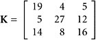
The determinant is 19, and the matrix is invertible by Theorem 5. Because Det(A) ≠ 0, the set of columns in A is linearly independent. As an alternative, we can compute the determinant from the upper-triangular echelon form that results from the row-reduction process:
 |
|
Again, the determinant is nonzero, and, by Theorem 4, the rows of this matrix form a linearly independent set.
SOLUTION The matrix in Example 6 is invertible (nonsingular) because its determinant is nonzero. The matrix in Example 7 is noninvertible (singular) because its determinant is 0.

SOLUTION We happen to notice that row 4 is the sum of rows 1, 2, and 3. Thus, if we subtract rows 1, 2, and 3 from row 4, the result is that row 4 becomes a zero row. Hence, the determinant will be zero, and the matrix is noninvertible by Theorem 5 (or by various other theorems).
Calculating Areas and Volumes
An application of determinants occurs in calculating the area of a triangle in ![]() . (The theory extends to volumes of three-dimensional figures and similar applications in still higher dimensions.) If the triangle has one of its vertices at 0, then we label the other two vertices as u and v. The notation Δ (0, u, v) specifies a triangle having vertices at 0, u, and v.
. (The theory extends to volumes of three-dimensional figures and similar applications in still higher dimensions.) If the triangle has one of its vertices at 0, then we label the other two vertices as u and v. The notation Δ (0, u, v) specifies a triangle having vertices at 0, u, and v.
THEOREM 6
In ![]() , if a triangle has vertices 0, u, and v, then the area of the triangle is one-half of the absolute value of the 2 × 2 determinant having rows (or columns) u and v.
, if a triangle has vertices 0, u, and v, then the area of the triangle is one-half of the absolute value of the 2 × 2 determinant having rows (or columns) u and v.
|
PROOF In general, a triangle whose vertices in ![]() are u, v, and w will be denoted by Δ (u, v, w). In the present situation, we note first that Δ(0, u, v) has the same area as Δ(0, u, v + λu), for any scalar λ. This is true because the two triangles have the same base and the same altitude (height). (See Figure 4.1 to convince yourself of this.) Recall that the area of a triangle is one-half the base, b, times the altitude (height), h, or Area [Δ(u, v, w)] =
are u, v, and w will be denoted by Δ (u, v, w). In the present situation, we note first that Δ(0, u, v) has the same area as Δ(0, u, v + λu), for any scalar λ. This is true because the two triangles have the same base and the same altitude (height). (See Figure 4.1 to convince yourself of this.) Recall that the area of a triangle is one-half the base, b, times the altitude (height), h, or Area [Δ(u, v, w)] = ![]() bh. Now apply, to the matrix in the statement of the theorem, the row operations of interchanging rows and adding a multiple of one row to another, ending with a diagonal matrix. For example, if u1 ≠ 0 we can write
bh. Now apply, to the matrix in the statement of the theorem, the row operations of interchanging rows and adding a multiple of one row to another, ending with a diagonal matrix. For example, if u1 ≠ 0 we can write

FIGURE 4.1 Triangles having the same base and altitude (height).
 |
|
Here we have used Property II twice and Property I once. Furthermore, we have
|
Figures 4.2 to 4.4 show the details of moving the vertices without changing the areas of the triangles. In going from Figure 4.2 to Figure 4.3, the vector v moves along a line parallel to u into a new position v′ on the vertical axis. In going from Figure 4.3 to Figure 4.4, u moves on a line parallel to v′ into a new position u′ on the horizontal axis. These motions do not affect the area of the triangle. (Explain why.) As shown in Figure 4.4, Δ(0, u′, v′) is a right triangle because one vertex u′ = (u1, 0) is on the horizontal axis and another ![]() is on the vertical axis. So the area of each of these triangles is
is on the vertical axis. So the area of each of these triangles is ![]() .
.
EXAMPLE 11
What is the area of the triangle whose vertices are (0, 0), (2, 11), and (8, 3)? Find the answer using determinants and then obtain the answer by drawing a sketch and using right triangles.
SOLUTION The area is one-half the absolute value of the determinant having rows (2, 11) and (8, 3):
|
Hence, the area sought is 41. To compute this area in another way, we draw a rectangle (with sides parallel to the coordinate axes) that contains the triangle in question. This rectangle will have area (8)(11) = 88. Next we remove three right triangles to leave only the triangle of interest. These triangles have areas 11, 12, and 24. Their total is 47, and 88 − 47 = 41. See Figure 4.5.
EXAMPLE 12
What is the area of the triangle whose vertices are (4, 7), (−2, 11), and (12, −6)?

FIGURE 4.2 Step 0: Triangles having the same base and altitude.

FIGURE 4.3 Step 1: Move v, parallel to u, into the new position v′ = (0, v2).

FIGURE 4.4 Step 2: Move u vertically into the new position u′ = (u1, 0).
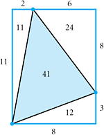
FIGURE 4.5 Triangle in a rectangle.
SOLUTION Because the triangle does not have a vertex at the origin, we simply subtract a fixed vector from each point of the object so that the new triangle has a vertex at 0. Thus, with a rigid motion, we can move this triangle so that one of its vertices is (0, 0). For example, subtract (4, 7) from each vertex, getting new vertices (0, 0), (−6, 4), and (8, −13). Then use the determinant formul a to obtain
|
THEOREM 7
The area of a parallelogram generated by the three points 0, u, and v in ![]() is the absolute value of the determinant having rows (or columns) u and v.
is the absolute value of the determinant having rows (or columns) u and v.
|
PROOF This follows from Theorem 6, because the parallelogram can be thought of as consisting of two congruent triangles.
In Section 4.2 (Theorem 3), we learn that a matrix and its transpose have the same determinant. Consequently, in Theorems 6 and 7, the areas of a triangle or parallelogram are unchanged by using column vectors instead of row vectors.
THEOREM 8
Let S be a triangle or parallelogram in ![]() having a vertex at 0. Let T be a linear mapping from
having a vertex at 0. Let T be a linear mapping from ![]() to
to ![]() , given by matrix A, so that T(x) = Ax. Then
, given by matrix A, so that T(x) = Ax. Then
|
PROOF If S is a parallelogram having vertices 0, u, v, and u + v, then by Theorem 7, the area of S is | Det[u, v] |. The parallelogram T(S) has vertices 0, T(u), T(v), and T(u + v), or, in other terms, 0, Au, Av, and Au + Av. Its area is
|
EXAMPLE 13
Let T(x) = Ax where ![]() . Let the vertices of a parallelogram S be (0, 0), (2, 5), (7, 3), and (9, 8). What is the area of T(S)?
. Let the vertices of a parallelogram S be (0, 0), (2, 5), (7, 3), and (9, 8). What is the area of T(S)?
SOLUTION By Theorem 8, we have
 |
|
Alternatively, we see that the new parallelogram has vertices
|
Thus, the area of the new parallelogram is
|
Mathematical Software
We can use mathematical software to evaluate determinants. For example, we can compute the determinant of a typical 4 × 4 matrix by using these commands in MATLAB, Maple, or Mathematica:
|
|
SUMMARY 4.1
• Det(U) = u11u22 ··· unn if U is an n × n triangular matrix.
• Det(A) =Det(Ã) if à is obtained from A by adding a multiple of one row onto another row.
• Det(A) =(1/c) Det(Ã) if à is obtained from A by multiplying a row of A by a constant c.
• Det(A) = − Det(Ã) if à is obtained by swapping a pair of rows in A.
• There is one and only one determinant function satisfying the rules I, II, and III.
• ![]()
• Det(A) = 0 if and only if A is singular. (Equivalently, the rows of A form a linearly dependent set.)
• The matrix A is noninvertible (singular) if and only if Det(A) = 0.
• The area of the triangle in ![]() having vertices 0 = (0, 0), u = (u1, u2), and v = (v1, v2) is
having vertices 0 = (0, 0), u = (u1, u2), and v = (v1, v2) is
|
• The area of a parallelogram in ![]() generated by points 0 = (0, 0), u = (u1, u2), and v = (v1, v2) is
generated by points 0 = (0, 0), u = (u1, u2), and v = (v1, v2) is
|
• If S is a triangle or parallelogram in ![]() with a vertex at 0 and if T is a linear transformation
with a vertex at 0 and if T is a linear transformation ![]() given by T(x) = Ax, then Area[T(S)] = | Det(A)| · Area(S).
given by T(x) = Ax, then Area[T(S)] = | Det(A)| · Area(S).
KEY CONCEPTS 4.1
Determinant of a matrix, computing determinants using standard row operations (replacement, scale, swap), determinant of triangular matrices, formula for the determinant of a 2 × 2 matrix, a matrix whose columns form a linearly dependent set has determinant 0, every noninvertible (singular) matrix has determinant 0, computing determinants without scaling, using row operations to evaluate determinants, calculating areas of triangles and parallelograms
GENERAL EXERCISES 4.1
1. Calculate the determinants of these matrices:
a. 
b. 
c. 
d. 
2. Let ![]()
For what values of the parameter β will the system have a unique solution?
3. Find the area of a triangle whose vertices are (−1, 3), (−4, −4), and (5, −2).
4. Consider 
Determine whether A is invertible or noninvertible by applying the determinant test.
5. Let 
Determine whether the rows of A form a linearly independent set by using the determinant criterion.
6. Verify that these four points are coplanar by showing that the parallelepiped having these vertices has volume 0: (0, 0, 0), (3, 2, 1), (4, −1, 2), and (6, −7, 4).
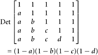
7. Compute Det 
8. Use the determinantal criterion for noninvertibility (singularity) to find all the values of t for which the matrix ![]() is noninvertible (singular).
is noninvertible (singular).
9. Find the value of x so that
Det ![]()
10. Let 
Determine whether the rows of A forma linearly dependent set. If so, find the coefficients involved in a linear combination of rows that is zero. Use the techniques in Section 1.3.
11. Let 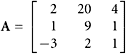
Using Properties I, II, and III and Theorem 1, calculate the determinant of A.
12. Let 
Compute the determinant of A by using the row replacement operations only (no scaling or swapping).
13. Let 
Compute the determinant of A by using row operations.
14. Let 
Compute the determinant of A by row operations leading to an upper triangular matrix.
15. Consider ![]()
Use the determinantal criterion for noninvertibility (singularity) to find all the values of t for which this matrix is noninvertible (singular).
16. Compute the determinant of 
17. Find the area of a parallelogram whose vertices are (0, 0), (3, 7), (4, −1), and (7, 6).
18. Compute Det 
19. Calculate Det  using two different sets of elementary operations.
20. Using determinants, find the area of the triangle and the parallelogram formed by the origin and these vectors:
a. x = (5, 3), y = (4, 7)
b. x = (−4, 3), y = (−2, 6)
21. We shall see later that a determinant is a linear function of any one of its rows. Consider a 2 × 2 matrix ![]() and prove that these are linear functions:
and prove that these are linear functions:
|
22. We shall establish later that the formula Det(AB) = Det(A) Det(B) is universally true. Explain it for the 2 × 2 case.
23. If the entries of a matrix are integers, does it follow that the determinant is an integer? A proof or an example is needed. Answer the analogous question for rational numbers.
24. The formula for the area of a parallelogram implies the formula for the area of a triangle, and vice versa. Another way to arrive at the area formula for a triangle is discussed in this problem. First draw a figure for a typical case as guidance. For example, plot these points in the plane: o = (0, 0), a = (3, 5), b = (6, 2), a′ = (3, 0), and b′ = (6, 0). Let us use the traditional method of describing polygons by listing their vertices, in order. We wish to calculate the area of the triangle oab (see Dörrie H. [1940]). We observe that the area of the quadrilateral oabb′ is the sum of the triangular area oaa′ and the trapezoid aa′b′b. Each of these two areas just mentioned is easily calculated because the altitudes are measured on horizontal lines. The area we want is the area of oabb′ minus the area of the triangle obb′. Carry out the calculation that leads to
![]()
Here a = (a1, a2) and b = (b1, b2).
25. Explain why if a parallelogram in the plane has integers for all the coordinates of its vertices, then its area is an integer.
26. Is there an equilateral triangle in the plane all of whose vertices have integer coordinates? If you can, answer the same question for vertices required to have rational coordinates.
27. A parallelogram has vertices (0, 0), (u1, u2), (v1, v2), and (u1 + v1, u2 + v2). What is its area?
28. Derive the formula for the area of a triangle by moving u parallel to v to a new position on the horizontal axis. Then move v horizontally to a position on the vertical axis.
29. In ![]() , the analog of a parallelogram in
, the analog of a parallelogram in ![]() is a parallelepiped. A cube is one example of this. A parallelepiped can be described by giving four vertices. A cube, for example, can be described by specifying these vertices: (0, 0, 0), (1, 0, 0), (0, 1, 0), and (0, 0, 1). Let a parallelepiped be described by giving these vertices: 0, u, v, and w. We accept without proof the fact that the volume of that figure is | Det(u, v, w)|. (The formula is certainly correct if u = (a, 0, 0), v = (0, b, 0), and w = (0, 0, c).) Find the volume of the parallelepiped having vertices (0, 0, 0), (2, 3, 4), (1, −1, 2), and (3, 0, 5).
is a parallelepiped. A cube is one example of this. A parallelepiped can be described by giving four vertices. A cube, for example, can be described by specifying these vertices: (0, 0, 0), (1, 0, 0), (0, 1, 0), and (0, 0, 1). Let a parallelepiped be described by giving these vertices: 0, u, v, and w. We accept without proof the fact that the volume of that figure is | Det(u, v, w)|. (The formula is certainly correct if u = (a, 0, 0), v = (0, b, 0), and w = (0, 0, c).) Find the volume of the parallelepiped having vertices (0, 0, 0), (2, 3, 4), (1, −1, 2), and (3, 0, 5).
30. (Continuation.) Use the information about parallelepipeds in the preceding problem. Find the volume of the parallelepiped whose vertices are (1, 2, −3), (2, 2, 1), (2, 3, 5), and (3, 0, 2).
31. Let u = (u1, u2), v = (v1, v2), p = (u1, v1), and q = (u2, v2). Do the triangles Δ(0, u, v) and Δ(0, p, q) have the same area? (Verify or give a counterexample.) Draw the triangles involved here in a concrete case, such as u = (5, 1) and v = (4, 3), and compute the two areas in question.
32. Refer to the proof of Theorem 6. Establish that the description of v′ is correct if we write it as v + tu where t = −v1 = u1.
33. (Continuation.) Use the same strategy to get a formula for the area, but begin by moving u parallel to v into a position on the first coordinate axis.
34. Explain why a 2 × 2 matrix A has this property: Det(αA) = α2 Det(A) for α, a scalar. Then prove the corresponding result for n × n matrices.
35. Critique this proof that every nonsquare matrix is invertible: Let A be a nonsquare matrix. Then A does not have a determinant. Hence, its determinant is certainly not zero. Now apply the theorem that asserts that a matrix is invertible if and only if its determinant is not 0.
36. Explain why 
is the area of a triangle whose vertices are three points u, v, w in ![]() . (Hint: Move the triangle rigidly so that one vertex becomes the origin, and then apply the formula already established.)
. (Hint: Move the triangle rigidly so that one vertex becomes the origin, and then apply the formula already established.)
37. Establish that 
is the equation of a line in ![]() passing through two distinct points v and w.
passing through two distinct points v and w.
38. What happens in Theorem 6 when vectors u and v are multiples of each other? What happens when u1 = 0?
39. Establish that if a 2 × 2 matrix is invertible (nonsingular), then by changing one entry in the matrix we can make it noninvertible (singular).
40. Explore another approach to determinants that uses these axioms:
I. Det(A) depends linearly on row 1.
II. Det(A) changes sign when two rows are swapped.
III. Det(I) = 1.
See Strang [2003].
41. Derive the formula for the determinant of a 2 × 2 matrix based on assuming a = 0 and a ≠ 0.
42. Explain why the proof of Theorem 8 is correct when S is a triangle.
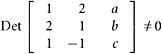
43. Consider ![]()
Find all values of the parameter β for which the matrix is invertible.
44. Find the area of the triangle whose vertices are given:
a. (0, 0), (−2, 2), (4, −1)
b. (1, −1), (5, −5), (7, −3)
45. Find the values of the unknowns when:
a. 
b. 
46. Show that
a. 
b. 
is the equation of the line in ![]() through point (x0, y0) with slope m.
through point (x0, y0) with slope m.
c. 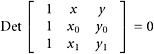
is the equation of the line in ![]() through distinct points (x0, y0) and (x1, y1).
through distinct points (x0, y0) and (x1, y1).
47. Find all values of x and y so that this matrix is not invertible.
|
48. Determine values of the integer n so that
|
49.
a. Describe the conic section when
 |
|
b. Under what conditions on the parameters a, b, and c do we have
 |
|

COMPUTER EXERCISES 4.1
1. Show that 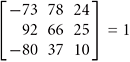 .
.
Explore how changing only one entry in this matrix by adding 0.01 to it affects the value of the determinant. For example, 92 ← 92.01 or 78 ← 78.01 or 10 ← 10.01. Would you expect the value of the determinant to change very much? Explain what happens.
2. Let A =(aij) be the n × n matrix defined by aij = |i − j|. Using various values of n, numerically determine if this formula is correct: Det(A) = (−1)n−1 2n−2(n − 1). For example, with n = 2, ![]() .
.
3. Consider the n × n matrix
 |
|
Using various values of n, r, and s, numerically determine if Det(A) = rn−1(r + ns).
For example, if n = 3, r = 2, s = 1, then
 |
|
4. Let 
Using various values of n, numerically determine whether
Det(A) = −n(n + 1)(2n − 5)/6.
For example, if n = 4, then
Det(A) = −10.
5. Compute the numerical values of each:
a. 
b. 
c. 
d. 
4.2 DETERMINANTS: PROPERTIES
No human investigation can be called real science if it cannot be demonstrated mathematically.
—LEONARDO DA VINCI (1452–1519)
Like the crest of a peacock so is mathematics at the head of all knowledge.
—AN OLD SAYING FROM INDIA.
In this unit, the determinant function will be further explored and more of its important properties will be revealed. Recall that in Section 4.1, we started with three important properties of this determinant function. These led to an algorithmic definition. Another definition can be given, of a completely different type. For us, this alternative definition is logically a theorem, because we have already defined determinants. This theorem leads to another algorithm for computing determinants, and it has many other applications.
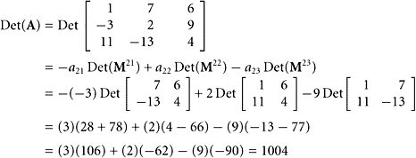
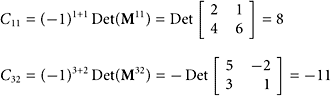
Minors and Cofactors
If A is an n × n matrix (where n ≥ 2), we can form submatrices of A by deleting one column and one row. The resulting (n − 1) × (n − 1) matrix is called a minor of the original matrix A. Let us denote by Mij the minor resulting from the removal of row i and column j from A. If we want to emphasize that the minor comes from the matrix A, we can write Mij(A), which is an (n − 1) × (n − 1) matrix.

SOLUTION We have
|
The next theorem shows how to compute determinants numerically by using a recursive algorithm. This method can be useful for small matrices, but it is inefficient for large matrices. See the following comments.
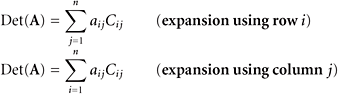
We will not prove this theorem but prefer simply to adopt it. The two formulas show how the determinant of an n × n matrix can be computed as a linear combination of determinants of (n − 1) × (n − 1) matrices. For that reason, the preceding formulas can be used in a recursive definition of determinants. A number of textbooks follow this route. See, for example, Andrilli and Hacker [2003] and Lay [2003]. The reader should note that the preceding displayed formulas are 2n in number, because the indices i and j can range over the integers from 1 to n.
EXAMPLE 2
In computing the determinant of a 6 × 6 matrix A = (aij), show the first step in the expansion using the fourth column.
SOLUTION First, we show the signs in the expansion going down column 4:
 |
|
To calculate the determinant of this matrix, we begin with
|
SOLUTION Because n = 3 in this example, there are six different applicable formulas in Theorem 1. For instance, we can use the first formula with i = 2, and apply it to the matrix A. If it is not ambiguous, we write Det A in place of Det(A).
 |
|
DEFINITION
The first formula in Theorem 1 is called a cofactor expansion of Det(A) using row i, and the second formula is a cofactor expansion of Det(A) using column j. The term cofactor applies to the quantities
|
Because we are denoting the cofactors by Cij, the formulas in Theorem 1 take this simpler form:
THEOREM 1′
Let A be an n × n matrix whose cofactors are denoted by Cij. Then these formulas are valid:
 |
|
Notice that the terms Mij are matrices of size (n − 1) × (n − 1), whereas the terms Cij are numbers. The cofactor matrix C having elements Cij is of some interest, as we shall see later. (It is almost the inverse of the matrix A!)
In some examples, the presence of zeros in strategic places can make the calculation of a determinant very easy. Here is one case of this phenomenon:

SOLUTION In this calculation, we used alternately a column expansion and a row expansion. We are free to do so, since Theorem 1 asserts the validity of both types of expansion on the successive matrices.
 |
|
Work Estimate
The cost of evaluating the determinant of an n × n matrix A using cofactor expansions is taken to be the number of long operations (multiplications). It can be denoted by f(n). We can show that
|
If A is 1 × 1, then f(1) = 0, since Det(A) = a11 and no arithmetic is needed. If A is 2 × 2, then expanding using the first row, we have Det(A) = a11C11 + a12C12 = a11a22 − a12a21 and f(2) = 2. If A is 3 × 3, then again expanding along the first row, we have Det(A) = a11C11 + a12C12 + a13C13. Hence, we obtain f(3) = 3f(2) + 3 = 9, since there are three matrices of order two and three multiplications. In general, it follows that f(n) = nf(n − 1) + n and f(n) ≈ nf(n − 1).
The amount of work involved in evaluating an n × n determinant using the recursive algorithm quickly becomes excessive. If we count only the multiplications and ignore the additions, we quickly reach astronomical levels of arithmetic! Let f(n) be the number of multiplications involved in computing the determinant of an n × n matrix using cofactor expansions. Then f(2) ≥ 2, f(3) ≥ 9, and f(n) ≥ nf(n − 1) + n. Using that inequality repeatedly, one obtains the lower bound
|
This is the nth factorial function.
The burden of work is overwhelming when n is large. For example, when n = 25, we obtain f(25) > 25! ≈ 1025. Suppose that we have a computer that can perform 1 trillion operations per second (1 teraflop per second). How long will this computer take to compute 1025 operations? It will take 1025 ÷ 1012 = 1013 seconds. Converting from seconds to years, we find that it would take 300,000 years to finish 1025 operations even with such a supercomputer. (Life is too short to wait for the results!)
Of the various ways to compute the determinant of a matrix, the method using row operations (Gaussian elimination) involves much less work than other methods. It requires approximately ![]() long operations. For example, with n = 25, this is about 5212, not 1025.
long operations. For example, with n = 25, this is about 5212, not 1025.
Direct Methods for Computing Determinants
Direct application of the formulas in Theorem 1 gives us the special formula for a 2 × 2 matrix:
|
Here, we have used the first of the two formulas in the theorem, and have taken i = 1. But there are three other choices we could have made, each leading to the same formula. Figure 4.6 illustrates the direct evaluation of a 2 × 2 determinant.

FIGURE 4.6 Direct evaluation of a 2 × 2 determinant.
Similarly, we can get the determinant of a 3 × 3 matrix:
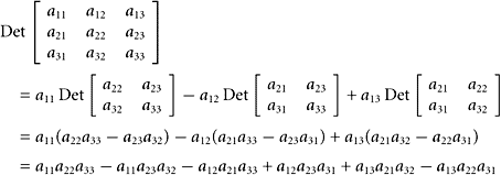 |
|
There are six different row and column expansions of a 3 × 3 matrix. It is a miraculous fact that all six lead eventually to the same formula. (That is, each formula should be expressed in simple form, as previously, without any 2 × 2 determinants and without parentheses.) The determinant of a 3 × 3 matrix can be calculated quickly via direct methods. Figure 4.7(a) illustrates the direct evaluation of a 3 × 3 determinant in a round-robin fashion: follow the arrows, multiply the elements together, and then add or subtract them according to the sign. Figure 4.7(b) is an alternative version of this method. There are no such simple algorithms for determinants of order greater than 3.
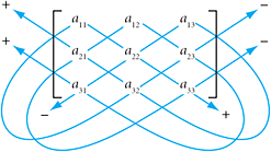
FIGURE 4.7(a) First version for the direct evaluation of a 3 × 3 determinant.

FIGURE 4.7(b) Second version for the direct evaluation of a 3 × 3 determinant.
Properties of Determinants
We explore next the many ways in which determinants interact with the other topics in linear algebra. This theme will arise again in the study of eigenvalues in Section 6.1.
PROOF Remember from Section 1.1 that in verifying such a statement involving elementary row operations, only two types of row operations need be utilized. Consider the row operation of multiplying row k in A by a nonzero constant c. This is effected by multiplying A on the left by an elementary matrix, E. The matrices involved are
 |
|
We see that Det(E) = c, Det(E) Det(A) = c Det(A), and Det(EA) = c Det(A) = Det(E) Det(A). The remainder of the proofis left as General Exercise 39.
SOLUTION Evidently, we have
|
PROOF Case 1. Suppose that A is noninvertible. In this case, Det(A) = 0 and Det(A) Det(B) = 0. Thus, we have to prove that Det(AB) = 0. By Theorem 5 in Section 4.1, it suffices to prove that AB is noninvertible. If AB is invertible, then we can write (AB)(AB)−1 = I. Thus B(AB)−1 is a right inverse of A. This contradicts Theorem 2 in Section 3.2.
Case 2. Suppose that A is invertible. In this case, a sequence of row operations on A will lead to In. (Recall that this is how we usually calculate inverses.) Representing these row operations by elementary matrices, we can write EkEk−1 ··· E2E1A = I. The corresponding set of inverse row operations will lead from I to A. We write this as ![]() . Consequently, by Lemma 1, we obtain
. Consequently, by Lemma 1, we obtain
 |
|

SOLUTION Using row operations, we have
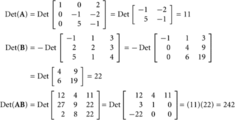 |
|
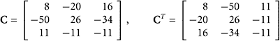
PROOF Write down the two matrices A and AT side by side. In A, be sure to show row j and column i. In AT, be sure to show column j and row i. These special rows and columns must be deleted to form Mij(AT) and Mji(A). After that deletion, the matrices that remain should be transposes of each other.
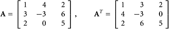
SOLUTION Use i = 3 and j = 2 in Lemma 2. Then
|
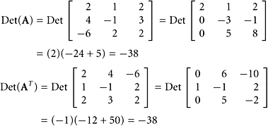
PROOF The theorem is certainly correct for 1 × 1 matrices. Proceeding by induction, we assume that the theorem has been established for all (n − 1) × (n − 1) matrices. Let A be an n × n matrix. By Lemma 2 and the induction hypothesis, we have, for any k,
 |
|
SOLUTION Again, using row operations, we obtain
 |
|
THEOREM 4
The determinant of a matrix is a linear function of any one column (or row).
PROOF We give the proof for the columns, and leave the other half to the exercises. The meaning of the first assertion in the theorem is this: Let A be an n × n matrix. Replace one column, say column j, by a variable vector, x = [x1, x2, …, xn]T. Call this new matrix Aj(x). Then x ![]() Det[Aj(x)] is a linear map from
Det[Aj(x)] is a linear map from ![]() to
to ![]() . To prove this, we expand Det[Aj(x + y)] by cofactors using column j:
. To prove this, we expand Det[Aj(x + y)] by cofactors using column j:
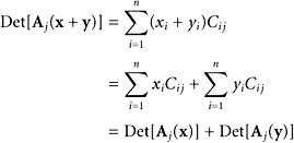 |
|
The other half of the linearity condition is similar and is left as General Exercise 40.
SOLUTION For column two, we obtain
 |
|
Cramer’s Rule
Systems of linear equations can be solved by using determinants and Cramer’s rule.1
THEOREM 5 Cramer’s Rule
If A is invertible, then the solution to the system of equations Ax = b is given by these formulas:
|
where Aj(b) is matrix A with its jth column replaced by b.
PROOF Denote the columns of A by a1, a2, …, an, and the columns of I by e1, e2, …, en. Use Ij(x) for the identity matrix with column j replaced by x. (We interpret x as a column vector.) Suppose that Ax = b. Then we have
|
Taking determinants, we have Det(A) Det[Ij(x)] = Det[Aj(b)]. This confirms the equation to be proved because Det[Ij(x)] = xj.

1Gabriel Cramer (1704–1752) was only 18 years old when he was awarded a doctorate. The theorem to which his name is attached is only one of his many accomplishments.
SOLUTION Cramer’s rule, with j = 2, leads to
 |
|
Planes in 
In three dimensions, the equation of a plane is
|
If three non-colinear points on a plane are given (x1, y1, z1), (x2, y2, z2), (x3, y3, z3), then the coefficients a, b, c can be found by these determinants
 |
|
which are parametric in d ≠ 0. Our remarks do not cover all cases. These equations can be found by using Cramer’s rule.
Computing Inverses Using Determinants
The inverse of a matrix can be computed directly using determinants and Cramer’s rule.
THEOREM 6
The inverse of an n × n invertible matrix A can be computed by the formulas
|
Here, as usual, Mji is the minor obtained from A by removing row j and column i and Cji = (−1)i+j Det(Mji) is the corresponding element of the cofactor matrix.
PROOF Fix an index j. We shall construct column j in A−1. Denote by x this column vector, which should satisfy the equation Ax = ej, where ej is the jth column in I. By Cramer’s rule, the components of the vector x are given by xi = Det[Ai(ej)]/Det(A), where Ai(ej) is the matrix that arises when we replace column i in A by the column-vector ej. To evaluate Det[Ai(ej)], perform a column expansion using column i. Because column i contains the vector ej, only one term emerges from the column expansion:
|
This calculation leads to
|
Recall the cofactors, Cij = (−1)i+j Det(Mij). By using cofactors, we obtain a simpler formula for the inverse:
|
where C is the cofactor matrix of A, having generic elements Cij. (The transpose of the matrix C is called the classical adjoint matrix of A: Adj(A) = CT. The term adjugate is also used.)

SOLUTION This matrix has nine cofactors, of which a small sample are given here:
 |
|
The matrix containing the cofactors and the transpose of that matrix are
 |
|
To finish this example, it is necessary to find the value of Det(A). An easy way to do this is to use the cofactor expansion and the matrices A and C. If we choose the top row of A, the corresponding cofactors will be the top row of C. (See Theorem 1'.) Thus, we obtain
|
We can verify this result with a direct calculation of the determinant of this 3 × 3 matrix
 |
|
The work can be verified in an independent manner by computing
 |
|
Notice that A · Adj(A) = Det(A)I.
Another interesting relationship between a matrix and its matrix of cofactors is given in the following theorem.
THEOREM 7
If the elements of one row in a matrix are multiplied by the cofactors of a different row and added up, the result is 0. Thus, if the matrix in question is A and if i ≠ j, then
|
A similar result is true for the columns of A; it is left to General Exercise 31.
PROOF Fix a pair (i, j) with i ≠ j, and form a matrix B, identical to A, except that the jth row of B is the ith row of A. Thus, B has two identical rows (namely rows i and j). Consequently, B is not invertible and has determinant 0. Notice that the minors of these two matrices obey this rule: Mjk(A) = Mjk(B), because A and B differ only in their jth rows, and these minors do not involve the elements in row j. Carry out a calculation of Det(B) by a row expansion using row j:
|
EXAMPLE 12
Let 
Multiply the entries in row two by the cofactors belonging to row one and add up the results, to see whether we get 0.
SOLUTION We have
 |
|
Vandermonde Matrix
The matrix that arises in the polynomial interpolation problem as described in Section 3.2, is called a Vandermonde matrix. If it involves n points, then its generic element is ![]() , where i and j run from 1 to n. It must be invertible, by Theorem 13, Section 3.2. As a matter of fact, the following theorem gives a formula for the determinant of the Vandermonde matrix.2
, where i and j run from 1 to n. It must be invertible, by Theorem 13, Section 3.2. As a matter of fact, the following theorem gives a formula for the determinant of the Vandermonde matrix.2
2Alexandre-Théophile Vandermonde (1735–1796) pursued a career as a violinist before turning to mathematical research and teaching. He was one of the first to study determinants as a worthwhile subject in itself.
The Π symbol on the right signifies the product of all factors (ti − tj), when 1 ≤ j < i ≤ n. The formula shows at once that the determinant is not zero and thus that the matrix is invertible.
Consider the 4 × 4 Vandermonde matrix
 |
|
The formula in Theorem 8 gives us
 |
|
EXAMPLE 13
Find the determinant of this matrix by using the preceding formula, and verify the answer by using appropriate row operations to simplify the work.
 |
|
SOLUTION We find
|
Application: Coded Messages
A simple way to send a secret message is to assign a different integer to each letter in the alphabet and send the message as the resulting string of integers. For simplicity, we assign the positive integers 1, 2, 3, …, 26 to the letters of the alphabet A, B, C, …, Z, in order, and use 27 for a space. Unfortunately, such a code is easy to break.However, matrix multiplication can be used to disguise the coded message further. We will use an integer matrix with determinant ±1. It has an inverse with integer entries. (See General Exercise 35.) Using such a matrix to transform the message makes it more difficult to decipher. To construct a coding matrix with determinant ±1, start with the identity matrix and apply swap and replacement operations with integer multipliers. For example, the message SEND HELP would be coded as [19, 5, 14, 4, 27, 8, 5, 12, 16]. Put the coded message into the columns of a matrix
 |
|
Using the following integer coding matrix N, which has Det(N) = −1, we compute the product
 |
|
Then the coded message SEND HELP would be [42, 103, 70, 47, 129, 86, 49, 126, 82]. The message received can be decoded by multiplying by the inverse of the coding matrix
 |
|
Once again, the coded message is contained in the columns of this matrix.
Mathematical Software
We can enter the data from Example 1 into the Maple system by using the following commands in Maple:
|
|
Also, we can verify the results in Example 7 by using these commands in Maple:
|
|
We can use Maple to check our results from Example 11.
|
|
Notice that Maple computes the classical adjoint.
Review of Determinant Notation and Properties
An n × n matrix has n2 minors. Each minor is obtained from A by removing one row and one column from A. Specifically, we denote by Mij or Mij (A) the minor resulting by the removal of the ith row and jth column from the matrix A. The cofactor associated with the minor Mij is defined to be the number Cij = (−1)i+j Det(Mij). These cofactors are therefore simple real numbers obtained by evaluating the determinants of the minors and inserting signs ± as indicated. We can then put these cofactors into a matrix C. An important relationship is ACT = Det(A)I. Thus, except for the factor Det(A), CT is the inverse of A.
SUMMARY 4.2
• A typical minor of A is Mij, obtained from A by removing row i and column j.
• A cofactor from A is anumber Cij = (−1)i+j Det(Mij).
• ![]() (cofactor expansion of Det(A) using row i.)
(cofactor expansion of Det(A) using row i.)
• ![]() (cofactor expansion of Det(A) using column j.)
(cofactor expansion of Det(A) using column j.)
• Det(AB) = Det(A) Det(B), where A and B are arbitrary n × n matrices.
• Mij(AT) = [Mji(A)]T
• Det(A) = Det(AT)
• Det(A) is a linear function of any one column (or row).
• (Cramer’s rule.) The solution of Ax = b is given by xj = Det[Aj(b)]/Det(A), where Aj(b) is obtained from A by replacing the jth column by b. (Here A is an n × n invertible matrix.)
• (A−1)ij = [(−1)i+j / Det(A)] Det(Mji) A−1 = (1/Det(A))CT
(Here A is an n × n invertible matrix.)
• ![]()
(If the elements of a row in A are multiplied by the cofactors of a different row and added, the result is zero.) A similar result is true for columns instead of rows.
• The Vandermonde matrix of order n is denoted by V and has generic elements ![]() , where 1 ≤ i, j ≤ n. The determinant of the nth order Vandermonde matrix is Det(V) = Π1≤j<i≤n (ti − tj)
, where 1 ≤ i, j ≤ n. The determinant of the nth order Vandermonde matrix is Det(V) = Π1≤j<i≤n (ti − tj)
• Summary of major properties:
•Det(AT) = Det(A)
•Det(A−1) = 1/Det(A)
•Det(AB) = Det(A) Det(B)
•Usually, Det(A + B) ≠ Det(A) + Det(B)
• Det(cA) = cn Det(A) if c ∈ ![]() and A is n × n.
and A is n × n.
• Det(A) = a11a22 ··· ann if A is upper or lower triangular.
• Det(Ã) = Det(A) if à results from A by a row-replacement operation.
• Det(Ã) = −Det(A) if à results from A by a row-swap operation.
• Det(A) = 0 if and only if the columns of A form a linearly dependent set. A similar result is true for the rows.
• Det(A) = 0 if and only if A is singular (not invertible).
KEY CONCEPTS 4.2
Minors, cofactors, row expansion, column expansion, Cramer’s rule, Vandermonde matrix
GENERAL EXERCISES 4.2
1. Let 
Establish that f is a linear function of x.
2. Use Cramer’s rule to solve the system  and b = [1, 1, 1]T
3. In Example 4, which numbers are involved in computing Det(A) and which are not?
4. Let 

Verify the assertion in Theorem 2 for this pair of matrices.
5. Find the inverse of the 3 × 3 matrix  by the formula in
Theorem 6. Along the way you may wish to use the minors of A, which are in the matrix 
6. Use Cramer’s rule to solve this system of equations:
 |
|
7. Use Cramer’s rule to solve this system:
 |
|
8. Compute  by cofactor expansions and by row operations.
9. Compute  by a cofactor expansion using row three and then column two.
10. In  , what are the minor M23, and the cofactor C23?
11. Compute 
by doing the following steps (in order): row operations using the pivot position (2, 3), cofactor expansion by the third column, and directly with a 3 × 3 matrix.
12. Let 
Verify Det(A) = Det(AT)
13. Let 

Verify Det(AB) = Det(A) Det(B)
14. Use Theorem 6 to compute inverses of these three matrices:
a. 
b. 
c. 
15. Using the cofactor matrices, compute the inverses of these matrices:
 |
|
16. Let 
Use Cramer’s rule to compute the (2, 3) entry of A−1.
17. Let 
Find the cofactor matrix C.
18. Use Cramer’s rule to solve this system:
 |
|
19. Let 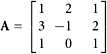
Express the inverse matrix in terms of the cofactor matrix. Verify the results by carrying out the multiplication ACT.
20. Using the direct method, compute
 |
|
21. Compute  by a direct method.
22. Consider 
Compute the determinant of this matrix using cofactor expansions.
23. Compute the determinant of
 |
|
24. Compute the determinant of
 |
|
25. Compute the determinant of
 |
|
26. Let 
Compute the determinant of A.
27. Explain why the determinant function is a linear function of any one row of the matrix on which it acts.
28. Let A be an n × n matrix, and fix two indices, p and q in the range from 1 to n. Replace apq by x. Now Det(A) is a function of the real variable x. What is the derivative of this function of x?
29. Explain why Det(ATB) = Det(A) Det(B).
30. Let A bean n × n matrix, where n is odd. Establish that if A is skew–symmetric (meaning AT = −A), then Det(A) = 0.
31. Establish the column version of Theorem 7.
32. The determinant of a general 3 × 3 matrix was computed in the text just before Theorem 2. Compute the same determinant by a column expansion using the third column and verify that the results are the same.
33. Let A be an arbitrary n × n invertible matrix. Explain why in each row there is an element that can be changed to make the matrix noninvertible.
34. Establish Theorem 7 by a direct calculation in this one case: Consider an arbitrary 3 × 3 matrix, and use the elements of row 2 and the cofactors belonging to row 3. Work out all the terms and see that they add up to 0.
35. Establish that if the entries in a square matrix A are integers and if Det(A) = ±1, then A−1 has the same two properties.
36. Explain why, for two n × n matrices, Det(AB) = Det(BA). Also, explain why this does not imply that AB = BA.
37. Establish that for arbitrary n × n matrices, Det(A1A2 … Ak) = Det(A1) Det(A2) … Det(Ak) using induction.
38. Give an argument why, for elementary matrices,
Det(E1E2 … Ek) = Det(E1) Det(E2) … Det(Ek).
39. Establish the one remaining case of Lemma 1.
40. Complete the proof of Theorem 4.
41. If we change one entry in a square matrix, will the determinant necessarily change? Give examples, and try to discover the theorems governing this question.
42. Establish that if A is invertible, then Det(A−1) = [Det(A)]−1. Find some other functions, f, for which Det[f(A)] = f[Det(A)]. To what extent are we limited to invertible matrices in this exploration?
43. Let A be an n × n matrix in which each entry has the form Aij = αijt + βij. What can you say about the determinant of A, as a function of t?
44. Find an example in which Det(A + B) ≠ Det(A) + Det(B). This will establish that Det is not linear. Reconcile this finding with Theorem 4.
45. Let A and B be n × n matrices such that Det(A) = 17 and Det(B) = 2. What are the numerical values of Det(AB), Det(BAT), Det(2A), Det(A−1), and Det(B2)?
46. Using determinants, prove that the product of two invertible n × n matrices is invertible.
47. Using Cramer’s rule, derive the equation ax + by + cz = d of a plane containing the three noncolinear points (x1, y1, z1), (x2, y2, z2), (x3, y3, z3) in which the coefficients a, b, c, d can be found by determinants.
48. Is the formula ![]() correct for the Vandermonde determinant? Explain why or why not.
correct for the Vandermonde determinant? Explain why or why not.
49. Suppose the vector w = (−1, 3, 7) is a linear combination of the vectors u = (4, 2, 7) and v = (3, 1, 4). When any one datum of this statement is altered, is it still true?
50. Determine which of the following inequalities are correct and which are incorrect:
a. ![]()
b. ![]()
c. ![]()
d. ![]() , |c| ≤ C, and |d| ≤ C
, |c| ≤ C, and |d| ≤ C
51.
a. To fit the data points (t0, y0) and (t1, y1) with the polynomial p(t) = a + bt, set up a linear system of equations and solve it using Cramer’s rule.
b. Repeat for the polymomial p(t) = c + d(t − t0). Hint: Use Cramer’s rule to solve the 2 × 2 system in Section 2.2 on linear least squares.
52. (Continuation.) Find the polynomial of the form p(t) = a + b(t − t0) + c(t − t0)(t − t1) that fits the data points (t0, y0), (t1, y1), and (t2, y2) using Cramer’s rule.
53. 
and C = AB. What is the numerical value of Det(C)?
COMPUTER EXERCISES 4.2
1. In an n × n Vandermonde matrix V, the (i, j)-element is ![]() . Use the symbol manipulation feature of Maple or Mathematica to obtain the general formula for the determinant of the 5 × 5 Vandermonde matrix. The n × n Vandermonde matrix is
. Use the symbol manipulation feature of Maple or Mathematica to obtain the general formula for the determinant of the 5 × 5 Vandermonde matrix. The n × n Vandermonde matrix is
 |
|
a. Devise a program for computing the determinant of an n × n Vandermonde matrix.
b. Use the Maple commands on page 288 to help you see a pattern in the factorization of the determinant of a Vandermonde matrix:
2. Using mathematical software, show that
 |
|
Show that this result holds true for matrices of various sizes. What conditions guarantee that the matrix is noninvertible?
3. Compute C−1 where
 |
|
4. Consider this n × n tridiagonal matrix
 |
|
Let dn = Det(Dn). For various values of n, verify numerically that d1 = 2, d2 = 3, and dn = 2dn−1 − dn−2 for n ≥ 3. Moreover, we obtain dn = n + 1.
5. Consider this n × n matrix
 |
|
For various values of n, verify numerically that
 |
|
6. Compute Det(A3(b)) where
 |
|
Then use Cramer’s Rule (Theorem 5) to compute x3 for the linear system Ax = b.