

Ask anyone on the street, and they'll tend to agree with you. Bigger is better. Get more bang for the buck. He who dies with the most toys wins. It stands to reason that, in most cases, more is better than only one. If one is good, two must be great.
It comes as no surprise, then, that computing has followed this trend from its infancy. Why even the ENIAC, widely regarded as the world’s first computer, didn’t have just a few parts. It had 19,000 vacuum tubes, 1,500 relays, and hundreds of thousands of resistors, capacitors, and inductors (http://ftp.arl.army.mil/∼mphist/eniac-story.html). Why did the founders use so many parts? If you had a device that could add two numbers together, that would be one thing. But given the budget, why not add three or even four together? More must be better.
As time went on and computing started to mature, the “more is better” approach seemed to function quite well. Where one processor worked well, two processors could at least double the processing power. When computer manufacturers started making larger and more efficient servers, companies could use the increased horsepower to process more data. It became evident early on that more processors equaled more computing power. Even with the advent of Intel’s 386 processor, magazines reported that a single computer could handle the workload of 15 employees!
The descendants of ENIAC were monster computers in their own right, although as we know, with the advent of the transistor, the parts inside got smaller and smaller. More parts were added to machines the size of refrigerators to make them faster, yet these supercomputers were out of the financial reach of most corporations. It didn’t take long to realize (okay, it happened in the 1990s) that supercomputer-like performance also could be achieved through a number of low-cost personal computers. More computers were better indeed—or simply cost much less.
Today’s computing environments require the needs of many computers to solve the tasks that only one wouldn’t be able to handle. Today’s large-scale computing environments involve the use of large server farms, with each node connected to each other in a clustered environment. The ASCI Project (Accelerated Strategic Computing Initiative), for instance, consists of several different clustered environments in a bid to provide “tera-scale” computing. ASCI White, capable of 12 trillion calculations per second, runs on IBM’s RS/6000 hardware and is becoming increasingly typical of solutions to large-scale computing problems. The ASCI plant at Sandia National Laboratories is comprised of Linux machines that run on Intel hardware and are part of the growing trend to emulate supercomputer performance.
Clustered computing, at its most basic level, involves two or more computers serving a single resource. Applications have become clustered as a way of handling increased data load. The practice of spreading attributes from a single application onto many computers not only improves performance, but also creates redundancy in case of failure. A prime example of a basic cluster is the Domain Name Service (DNS), with its built in primary, secondary, and cache servers. Other protocols have also built in clustered/redundancy characteristics, such as NIS and SMTP.
Although clustering might not be a panacea for today’s ills, it might help the organization that is trying to maximize some of its existing resources. Although not every program can benefit from clustering, organizations that serve applications, such as web servers, databases, and ftp servers, could benefit from the technology as loads on the systems increased. Clusters can easily be designed with scalability in mind; more systems can be added as the requirements increase, which spreads the load across multiple subsystems or machines.
Entities that require a great deal of data crunching can benefit from high-performance computing, which greatly reduces the amount of time needed to crunch numbers. Organizations such as the National Oceanic and Atmospheric Administration are able to use clusters to forecast trends in potentially deadly weather conditions. The staff at Lawrence Livermore Lab use clustered computers to simulate an entire nuclear explosion without harm to anyone (except the backup operators who have to maintain all that data).
Companies serving a great deal of bandwidth can benefit from load-balanced clusters. This type of cluster takes information from a centralized server and spreads it across multiple computers. Although this might seem trivial at first, load balancing can take place in a local server room or across wide-area networks (WANs) spanning the globe. Larger web portals use load balancing to serve data from multiple access points worldwide to serve local customers. Not only does this cut down on bandwidth costs, but visitors are served that much more quickly.
These load-balanced servers also will benefit from the High Availability (HA) model. This model can include redundancy at all levels. Servers in a HA cluster benefit from having two power supplies, two network cards, two RAID controllers, and so on. It’s unlikely that all the duplicate devices of a HA cluster will fail at once, barring some major catastrophe. With the addition of an extra component to the primary subsystem or the addition of an extra server, an extra component can be put in place to help in case of failover. This is known as N+1 redundancy and is found in clusters, RAID configurations, power arrays, or wherever another component can take over in case of failure.
With all the possible platforms from which you could choose, one might wonder why you would choose Linux as an operating system (OS) in which to house your critical applications. After all, with clustering being such a hot topic, each vendor has its own implementation of clustering software, often more mature than the homegrown efforts of dozens of programmers. All major OS vendors support clustering. Microsoft includes its clustering application directly into its Windows 2000 Advanced Server OS. Sun Microsystems offers its High Performance Cluster technology for parallel computing, as well as Sun Cluster for high availability. Even Compaq, Hewlett Packard, IBM, and SGI support clustered solutions.
So why are these companies starting to embrace Linux when they have their own product lines? With the exception of Microsoft, these vendors are starting to recognize the value of open source software. They realize that, by incorporating Linux into their business strategies, they’ll utilize the benefits of hundreds, if not thousands, of programmers scrutinizing their code and making helpful suggestions. Although open source methodology remains to be seen as a viable business model, large companies reap the socialistic benefits of having such a philosophy.
Linux runs on just about any hardware platform imaginable. Just as it’s proven to be more than capable of powering large mainframes and server farms as well as desktop machines, the versatile OS has been ported to hand-held devices, television recorders, game consoles, Amiga, Atari, and even Apple 040 computers. Linux is well known for being an easy-to-use commodity, off the shelf parts. Although the availability for Linux drivers might not be as prevalent as other operating systems, there is still plenty of hardware that works without a hitch. Linux also supports a great deal of legacy hardware, enabling older computers to be brought back into service. The creators of Linux even envision it as the premiere OS of embedded devices because the kernel can be modified in any shape or form. (Although Linus Torvalds invented Linux and holds the copyright, he didn’t write the entire thing himself.)
No other OS allows for this level of versatility. It’s this approach to modular computing that makes Linux perfect for clusters.
Although Linux has many advantages for clustering, it also has faults that might make it an unattractive solution for certain types of clusters. The bottom line is that Linux is a relatively new OS (albeit based on tried-and-true technologies). For the most part, you’ve got an OS written by volunteers in their spare time. Though the code is readily available for scrutiny by anyone, the thought does exist that top-notch programmers might be whisked away by companies that can afford to pay top salaries. (Of course, that does happen, and for some reason, programmers even manage to work on Linux with something called spare time.)
The level of support is not as robust as you can get with other operating systems. That isn’t to say that you can’t get good vendor support; on the contrary, the quality of support for Linux is top notch. There just isn’t as much support out there for the product as there is for other operating systems.
A few bugs are still inherent with the OS and kernel. The native file system, ext2, doesn’t support journaling. USB support has typically been spotty. There tends to be a smaller amount of drivers for Linux than there are for other operating systems, even though the most common solutions are addressed.
However, most, if not all, of these issues are being addressed. Robust file systems are available for Linux other than ext2, and support for USB is improving with each release (as of 2.2.18, anyway). Typically, most of these issues don’t come into play when you’re deploying large cluster farms. Most of these limitations will only be applicable when you use Linux on the desktop. But the development of the Linux kernel is rapidly outpacing the development of other operating systems as the developers strive to fix issues such as USB support.
The system administrator has to keep a sense of perspective when rolling out any OS. Linux is primarily a server class OS. It’s designed to handle large tasks supporting many users and processors, and it does that well. With the support of projects such as Gnome and KDE (not to mention every other window manager out there), Linux can be used primarily as a workstation in addition to a server. The development for Linux-based workstation class computers is more advanced than most other UNIX systems. However, both Macintosh and Microsoft tend to own more market share and usability than the rapidly advancing Linux desktop.
The loud hum of the air conditioning breathes through the massive data center as thousands of computers lie still in the darkness. The single green eye from the power switch illuminates racks upon racks of servers as far as the eye can see. Evocations of the giant machine are immediately brought to attention as the almost haunting image of a single entity bears down upon the onlooker.
Okay, so even though it’s not really such an ominous entity, the high performance cluster is arguably the most popular type known to the masses. Vector computing, a type of high-performance machine, tends to be cost prohibitive for commodity use due to the specialized hardware that it requires. Parallel computers, on the other hand, have become immensely popular due to the fact that almost anyone can build one with spare parts. The name Beowulf is almost as synonymous with parallel clustering as Jello is with flavored gelatin. Parallel computers have grown tremendously in popularity as researchers and hobbyists alike are able to mirror supercomputer performance. Of course, clustering doesn’t begin and end with the parallel or Vector computer.
So now that you have a basic understanding of the different types of clusters that we discuss in this book, I’m sure you’re asking, “Yes, that’s all well and good, but what does it all mean?” For that, you should consult your favorite religious text. For the person who is comfortable with his or her beliefs and wants to get in to the business of setting up Linux clusters, Chapter 2, “Preparing your Linux Cluster,” would be perfect. For the curious individual who wants to understand the theories behind clustering technologies, the rest of this chapter is for you.
Making two or more Linux machines interact with each other is quite easy. The simplest way is to assign each machine an IP address and a subnet mask, attach a crossover cable between them, and voila—instant network. Things start to get more complicated when there’s a few more machines involved, although it’s still not rocket science. Add another computer, and you have to add a switch or hub. Connect your computer to another network, and you have to add a router of some kind. Getting clustered computers to talk to each other at the most basic level is as simple as setting up a network. However, getting them to interact in different ways is another story.
Computers have an annoying tendency to break down when you least expect. It’s a rare find to come across a system administrator that hasn’t received a phone call in the middle of the night with the dreaded news that a critical system is down, and would you please attend to this situation at your own convenience (right now!).
The concept of highly available and fault-tolerant clusters tend to go hand in hand. If a system is going to achieve high uptimes, the more redundant subsystems it needs to remain operating—such as the addition of servers in a clustered configuration. The bottom line for high availability clusters is that the application is of such high importance that you take extra steps to make sure it’s available.
The single point of failure (SPOF) is a common theme in HA clusters. Having a single component is just asking for trouble, and the SPOF is a paradigm to be avoided at all costs. In a perfect world, each server would have a redundant subsystem for each component in case the primary died or stopped responding. Critical subsystems that usually fail include hard drives, power supplies, and network cards. It’s a sad fact of life, but user error tends to account for most downtime. Operators have been known to unmount volumes of critical live data, and contractors reorganize cables that are poorly labeled.
Such redundancy planning might include adding a RAID controller in case of hard drive failure, but what if the controller died? A whole different set of controllers and RAID devices could be implemented to reduce the risk of the SPOF. An architecture would have to be considered that would allow for hotswappable CPUs. Two network cards could be implemented in case connectivity problems become an issue. A network card could be tied to a different switch or router for backup. What then for the network itself? What if a switch went bad? A second switch then could be set in place in case the first one died, and then a redundant router, redundant network provider might all be considered. It’s a fine line between handling an SPOF and total redundancy of all systems, where budget is usually the deciding factor.
Achieving 100 percent uptime is near impossible, although with the right technologies, you can come quite close to that. A more realistic goal to set when planning a HA solution is providing for an uptime of 99 percent or higher. In doing so, you can plan scheduled downtime for maintenance, backups, and patches requiring reboots. Having an uptime requirement of greater than 99 percent requires different models, such as redundant systems.
Although there are servers designed with redundancy in mind, their prices tend to be much larger than SPOF servers. There are companies that develop servers with no SPOF, including two motherboards, two CPUs, two power supplies, and so on. These are even more expensive, but for the organization that can’t afford downtime, the cost to data integrity ratio evens out.
Fortunately, there is another way to achieve such redundancy without the high cost of redesigning single server architecture. Incorporating two or more computers achieves a second layer of redundancy for each component. There are just about as many ways to achieve this redundancy as there are people implementing servers. A backup server that can be put into production is among the most common methods that are currently implemented. Although this works in most environments, offline redundant servers take time to prepare and bring online. Having an online failover server, although more difficult to implement, can be brought up almost immediately to replace the initial application.
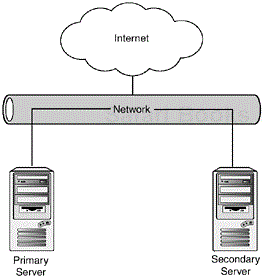
In Figure 1.1, two computers are connected to the same network. A heartbeat application that runs between them assures each computer that the other is up and running in good health. If the secondary computer cannot determine the health of the primary computer, that computer takes over the services of the primary. This is typically done with IP aliasing and a floating address that’s assigned with DNS. This floating address will fail over to the secondary computer as soon as the heartbeat detects an event such as the primary server or application failing. This method works well if all the served data is static. If the data is dynamic, a method to keep the data synched needs to be implemented.
Shared storage is the method where two or more computers have access to the same data from one or more file systems. Typically, this could be done through a means of shared SCSI device, storage area network, or a network file system. This would enable two or more computers to access the data from the same device, although having the data on only one device or file system could be considered an SPOF.
It’s no surprise to any of us that today’s mission-critical servers need access to data that’s only milliseconds old. This isn’t a problem when you have one server and one storage medium. Databases and web servers can easily gain access to their own file systems and make changes as necessary. When data doesn’t change, it’s not a problem to have two distinct servers with their own file systems. But how often do you have a database of nothing but static data? Enter shared storage and another server to avoid the SPOF. Yet that scenario opens up a new can of worms. How do two servers access the same data without the fear of destroying the data?
Let’s examine this scenario more closely. Imagine if you will, employees at XYZ Corporation who install a database server in a highly available environment. They do this by connecting two servers to an external file storage device. Server A is the primary, while server B stands by idle in case of failover.
Server A is happily chugging away when Joe Operator just so happens to stumble clumsily through the heartbeat cables that keep the servers synched. Server B detects that server A is down and tries to gain control of the data while the primary continues to write. In “high availability speech,” this is known as a split-brain situation. Voila—an instant recipe for destroyed data.
Fencing is the technology used to avoid split-brain scenarios and aids in the segregation of resources. The HA software will attempt to fence off the downed server from accessing the data until it is restored again, typically by using SCSI reservations. However, the technology has not been foolproof. With advances in the Linux kernel (specifically 2.2.16 and above), servers can now effectively enact fencing and, therefore, share file systems without too many hassles.
Although shared storage is a feasible solution to many dynamic data requirements, there are different approaches to handling the same data. If you can afford the network delay, a solution that relies on NFS, or perhaps rsync, could be a much cleaner solution. Shared storage, although it has come a long way, adds another layer of complexity and another component that could potentially go wrong.
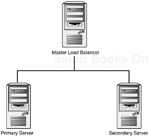
Load balancing refers to the method in which data is distributed across more than one server. Almost any parallel or distributed application can benefit from load balancing. Web servers are typically the most profitable, and therefore, the most used application of load balancing. Typically in the Linux environment, as in most heterogeneous environments, this is handled by one master node. Data is managed by the master node and is served onto two or more machines depending on traffic (see Figure 1.2). The data does not have to be distributed equally, of course. If you have one server on gigabit ethernet, that server can obviously absorb more traffic than a simple, fast ethernet node can.
One advantage of load balancing is that the servers don’t have to be local. Quite often, web requests from one part of the country are routed to a more convenient location rather than a centralized repository. Requests made from a user are generally encapsulated into a user session, meaning that all data will be redirected to the same server and not redirected to others depending on the load. Load balancers also typically handle failover by redirecting the traffic from the downed node and spreading the data across the remaining nodes.
The major disadvantage of load balancing is that the data has to remain consistent and available across all the servers, though one could use a method such as rsync to keep the integrity of data.
Although load balancing is typically done in larger ISPs by hardware devices, the versatility of Linux also shines here.
Programs such as Balance and the global load balancing Eddie Mission are discussed in Chapter 6, “Load Balancing.”
Take over three million users, tell them that they too can join in the search for extraterrestrial life, and what do you get? You get the world’s largest distributed application, the SETI@home project (http://setiathome.ssl.berkeley.edu/). Over 630,000 years of computational time has been accumulated by the project. This is a great reflection on the power of distributed computing and the Internet.
Distributed computing, in a nutshell, takes a program and assigns computational cycles to one or more computers and then reassembles the result after a certain period of time. Although close in scope to parallel computers, a true distributed environment differs in how processes and memory are distributed. Typically, a distributed cluster is comprised of heterogeneous computers, which can be dedicated servers but are typically end-user workstations. These workstations can be called on to provide computational functionality using spare CPU cycles. A distributed application will normally suspend itself or run in the background while a user is actively working at his computer and pick up again after a certain timeout value. Distributed computing resources can easily be applied over a large geographical area, constrained only by the network itself.
Just about any computationally expensive application can benefit from distributed computing. SETI@home, Render Farms (a cluster specifically set up to harness processing power to do large scale animations), take over three million users, tell them that they too can join in the search for extraterrestrial life, and what do you get? And different types of simulations can all benefit.
Parallel computing refers to the submission of jobs or processes over more than one processor. Parallel clusters are typically groups of machines that are dedicated to sharing resources. The cluster can be built with as little as two computers; however, with the price of commodity hardware these days, it’s not hard to find clusters with as little as 16 nodes or perhaps several thousand. Google has been reported to have over 8,000 nodes within its Linux cluster.
Parallel clusters have also been referred to as Beowulf clusters. Although not technically accurate for all types of HPCs, a Beowulf type cluster refers to “computer clusters built using primarily commodity components and running an Open Source operating system.”
Parallel computers work by splitting up jobs and doling them out to different nodes within the cluster. Having several computers working on a single task tends to be more efficient than one computer churning away on the same task, but having a 16-node cluster won’t necessarily speed up your application 16 times. Parallel clusters aren’t typically “set up and forget about them” machines; they need a great amount of performance tuning to make them work well. Once you’ve tuned your system, it’s time to tune it again. And then after you’ve finished that, it might benefit from some more performance tuning.
Not every program benefits from a parallel configuration. Several factors must be considered to judge accurately. For example, is the code written to work under several processors? Most applications aren’t designed to take advantage of multiple processors, so doling out pieces of your program would just be futile. Is the code optimized? The code might work faster on one node instead of splitting up each part and transferring it to each CPU. Parallel computing is really designed to handle math-intensive projects, such as plotting the expansion of the universe, render CPU-intensive animations, or decide exactly how many licks it actually takes to get to the center.
The parallel cluster can be set up with a master node that passes jobs to slave nodes. A master node will generally be the only machine that most users see; it shields the rest of the network behind it. The master node can be used to schedule jobs and monitor processes, while the slave nodes remain untouched (except for maintenance or repair). In a high production environment with several thousand systems, it might be cheaper to totally replace a downed node than to diagnose the error and replace faulty parts within the node.
Although several methods have been designed for building parallel clusters, Parallel Virtual Machine (PVM) was among the first programs to allow code to run across several nodes. PVM allows a heterogeneous group of machines to run C, C++, and Fortran across the cluster. Message Passing Interface (MPI), a relative newcomer to the scene, is shaping up to be the standard in message passing. Each is available for almost every system imaginable, including Linux.
Included within the Parallel Processing model exist cluster configurations called NOWs and COWs—or even POPs. Generally, the concept of a NOW and a COW can be synonymous with any parallel computer; however, there tends to be some disagreement among the hardcore ranks. A NOW is a network of operating systems, the COW is a cluster of operating systems, and a POP is a Pile of PCs (Engineering a Beowulf Style Computer Cluster, http://www.phy.duke.edu/brahma/beowulf_book.pdf). If one takes the approach that a parallel cluster is comprised of machines dedicated to the task of parallel computing, then neither a NOW nor a COW fit the bill. These typically are representative of distributed computing because they can be comprised of heterogeneous operating systems and workstations.
From the earliest days of computing, people would stare at their monitors with utter impatience as their systems attempted to solve problems at mind-bogglingly slow speeds (okay, even with modern technology, we still haven’t solved this problem). In 1967, Gene Amdahl, who was working for IBM at the time, theorized that there was a limit to the effectiveness of parallel processing for any particular task. (One could assume that this theory was written while waiting for his computer to boot.) More specifically, “every algorithm has a sequential part that ultimately limits the speedup that can be achieved by a multiprocessor implementation” (Reevaluating Amdahl’s Law by John L. Gustafson; www.scl.ameslab.gov/Publications/AmdahlsLaw/Amdahls.html). In other words, there lies certain parts to each computation, such as the time it takes to write results to disk, I/O limitations, and so on.
Amdahl’s Law is important in that it displays how unreasonable it is to expect certain gains above a typical threshold. Even though Amdahl’s Law remains the standard in demonstrating the effectiveness of parallel applications, the law remains in dispute and even begins to fall apart as larger clusters are becoming commonplace. According to John L. Gustafson in Reevaluating Amdahl’s Law:
“Our work to date shows that it is not an insurmountable task to extract very high efficiency from a massively-parallel ensemble. We feel that it is important for the computing research community to overcome the ‘mental block’ against massive parallelism imposed by a misuse of Amdahl’s speedup formula; speedup should be measured by scaling the problem to the number of processors, not fixing problem size.” (See On Microprocessors, Memory Hierarchies, and Amdahl’s Law; www.hpcmo.hpc.mil/Htdocs/UGC/UGC99/papers/alg1/).”
Although certain people dispute the validity of Amdahl’s Law, it remains an easy way to think about those limitations.
Symmetric multiprocessing (SMP) includes any SMP architecture. In layman’s terms, it’s a computer with more than one processor. SMP architectures differ from asymmetrical processing architectures primarily in the way that they can truly be considered multitasking rather than time-sharing devices. Any idle processor can be delegated to take on additional tasks or handle increased loads.
Generally, a well-written and optimized application performs much better on an SMP machine than on two or more computers with a single processor. Several factors determine the speed at which the application runs, including the speed of the motherboard bus, the memory, the speed of the drives, as well as the I/O throughput. Like the addition of more nodes for parallel computing, the programs have to be rewritten or optimized to enable multiple threads. Processes and kernel space threads are naturally distributed among SMP machines. User processes generally aren’t; however, the kernel does a sort of natural load balancing across each of the CPUs. Applications that can make use of fork() can benefit from an SMP architecture. fork() allows a process to split itself into two identical copies, which, depending on the OS, will share the same memory, yet will run on a different CPU. If the application is primarily CPU driven, that application will see benefits from the SMP architecture. However, the price for computers with more than one processor might outweigh the benefits of an SMP processor machine.
Linux added support for SMP with the addition of the 2.0 kernel, which included support for Intel 486 and higher (and clones), as well as hypersparc machines. With the addition of the 2.2 kernel, Linux added support for UltraSparc, SparcServer, Alpha, and PowerPC machines.
Although the 2.2.x and 2.4.x kernels’ SMP support is added by default, it can be added in with the following settings (the latest kernel can always be found at www.kernel.org, or at ftp://ftp.kernel.org/pub/linux/kernel):
Configure the kernel and answer “yes” to the question, “Symmetric Multi-Processing Support.”
Enable “Memory Type Range Register (MTRR) Support” (both under Processor Type and Features).
Enable real-time clock support by configuring the “RTC Support” item (under Character Devices).
On the x86 kernel, do not enable Advanced Power Management (APM). APM and SMP are not compatible, and your system will almost certainly crash while booting if APM is enabled.
You must rebuild all of your kernel and kernel modules when changing to and from SMP mode. Remember to make modules and make modules install. You can display the result with cat /proc/cpuinfo.
As previously mentioned, clusters are made up of two or more different machines (or processors) that serve the same application. Even though it takes a little more to make a full-fledged clustered solution for most applications, it’s easy to bring basic services to most networks.
All Linux actually needs to be involved in a cluster is to talk to other machines in a network, which includes most of the machines out there. Put two boxes together that talk to each other, and you have a cluster—not a very effective cluster, mind you, but one that works. It’s a simple matter, really, to enable basic clustering features to existing servers.
A basic HA cluster can be achieved with nothing more than straight ping. If you were to set up a script that would enable a failover server to ping a primary application server every minute or so, the failover server could determine when the primary failed. As soon as the secondary couldn’t find the other server, it would assume that it was down and launch scripts to enable its own services. After all, if the failover server can’t reach the primary, neither can any other service or user.
You need to consider some options before you start planning for your basic HA cluster. Are you going to have the failover server in standby mode with an application already running, ready to go? Is the standby server already in production with other elements running? Here’s what you need to set up a basic HA cluster:
Script that will ping the other server.
Crontab entry to call the script.
If the other server responds, then sleep.
If the other server doesn’t respond, ping again.
If the other server still doesn’t respond, assume failover sequence.
Take over IP address of failed server.
The first step when implementing such a cluster is to assign a virtual IP to the servers. This serves as the floating address that resolves to a DNS entry. Initially, the primary server owns the IP and then the secondary assumes it after failover.
IP aliasing has to either have been compiled in the kernel or have been loaded as a module. The kernel configuration for 2.2.x kernels is under Networking Options, IP: Aliasing Support, and is unchecked by default. Module support is only available in 2.0.x kernels. 2.2.x kernels either have support compiled in or not.
The module that you’ll be looking for is ip_alias. To insert it into the 2.0.x kernel, use the insmod command.
RedHat 7.1 default install allows for an IP alias right out of the box. A stock 6.2 does as well, yet Debian 2.2 doesn’t, so check your distribution.
After IP aliasing is available, an extra alias (or several) can be added with the same ease as a regular IP. The format is
/sbin/ifconfig <interface>:<virtual number> <ip> netmask <netmask> up
For example,
/sbin/ifconfig eth0:1 172.16.0.1 netmask 255.255.0.0 up
brings up virtual interface one and attaches it to adapter eth0 with an IP of 172.16.0.1 and a class B /16 netmask. Assign the virtual interface to the interface of the primary server and make sure that this entry is resolved by DNS.
The next step includes setting up the failover script. This script, placed on the failover server, initially pings the primary server and exits if a response is given. If a response is not given, the program waits for 20 seconds and pings again. If the failover server doesn’t receive a ping response from the primary a second time, the server then sets the virtual IP on itself and optionally sends out a notification. Don’t forget to set the script executable.
#!/bin/bash
# Poor Man's Cluster
# Script to Test for Failover
#
host="172.16.0.2"
netmask="255.255.0.0"
while true; do
/bin/ping -c 5 -i 3 $host > /dev/null 2>&1
if [ $? -ge 1 ]; then
        #This doesn't look good, let's test again.
        /bin/ping -c 5 -i 3 $host > /dev/null 2>$1
                if [ $? -ge 1 ]; then
                # We need to assume host is really down. Assume
                # failover sequence
                /sbin/ifconfig eth0:1 $host netmask $netmask up
                echo "$host is down. Please check immediately." > /bin/mail -
s "$host is down!" [email protected]
                else
                #second ping returned a value. Whew.
                :
else
:
fi
done
The script should be able to run in the background and mail the designated user if a connectivity problem occurs. The script can easily be adapted to ping more than one host, if you’re creative enough.
A quick and dirty way to enable load balancing can be achieved with simple A records in DNS. Although it presents itself as a dirty hack, enabling the same name with two or more different IP addresses does offer a measure of load balancing, albeit limited in scope. The same effect does not work, however, when enabling different IP addresses in /etc/hosts.
To illustrate, we have the following zone enabled:
[root@matrix named]# cat zone.dns
;
; Zone file for zone.com
;
@       IN      SOA     zone.com. postmaster.zone.com. (
                        19990913        ; serial
                        10800           ; refresh
                        3600            ; retry
                        604800         ; expire, seconds
                        86400 )         ; minimum, seconds
IN NS      ns1.zone.com.
IN NS      ns2.zone.com.
host1          IN A    10.2.2.10
host1          IN A    10.2.2.11
host1          IN A    10.2.2.12
In this example, each host carries the same domain name, yet the A record points to a different address. Pings of the machine show the following:
   [root@matrix named]# ping host1

PING host1.zone.com (10.2.2.10) from 10.2.2.100 : 56(84) bytes of data.
   [root@matrix named]$ ping host1

PING host1.zone.com (10.2.2.11) from 10.2.2.100 : 56(84) bytes of data.
   [root@matrix named]$ ping host1

PING host1.zone.com (10.2.2.10) from 10.2.2.100 : 56(84) bytes of data.
   [root@matrix named]$ ping host1

PING host1.zone.com (10.2.2.12) from 10.2.2.100 : 56(84) bytes of data.
As you can see, it’s not a foolproof situation, but it does offer some method of load balancing between hosts.
The second extended file system, ext2, was developed by René Card as an alternative to the first file system derived from Minix. Although Linux supports many different file systems, ext2 remains the default for most distributions. Many vendors have improved on the default file system to offer features such as journaling, volume management, network block file systems, and shared disk file systems. Ext2 does not have these features built in.
Enter the journal, the most popular alternative method to keep track of the file system. Depending on the implementation, journaling file systems use different methods based on a database to keep track of file system data. What’s so attractive about journaling file systems is that fsck isn’t needed. In the event of a system crash, the logs from the database can be replayed to represent the data at the time of a crash. This method tends to bring the system up to a consistent state much faster than a file system run with fsck; however, it doesn’t do anything special for data reliability. A large RAID device that’s using ext2 might take several hours to go through fsck checks, although with the addition of a journaling file system, no checks are made. All writes are made and played back from the journal, which results in a boot time of only minutes.
Different journaling file systems also have support for synchronous I/O, increased block size support, integration with NFS, quota support, and support for access control lists (ACLs).
Network file systems manage to take one or more devices and appear to the server as one logical volume. The trick here is to fool the OS into thinking that the volume is a locally attached RAID or clustered device. The network file system naturally shows some performance loss due to the network overhead.
Networking is an essential part of clustering. Computers just can’t talk to each other on their own; that would be creepy. Parallel networks need a dedicated networking environment, where in comparison, quite a few load balanced, distributed, and even some HA solutions are designed over a WAN environment. To better understand the relationship between the network and the cluster, we need to understand network issues and how they affect cluster communications. Although we won’t get into a detailed explanation of TCP/IP and networking, a cursory examination is provided here.
The International Organization for Standardization (ISO), an international body comprised of national standards bodies from more than 75 countries, created the Open Standards Interconnection (OSI) model in order for different vendors to design networks that would be able to talk to each other. The OSI model, finally standardized in 1977, is basically a reference that serves as a general framework for networking.
It wasn’t uncommon to find vendors about 30 years ago who produced computers that didn’t have the ability to talk to other vendors. Along with creating operating systems and mainframes that were rather proprietary, the communications of the time were mostly proprietary as well. In 1977, the British Standards Organization proposed to the ISO that an international standard for distributed processing be created. The American National Standards Institute (ANSI) was charged with presenting a framework for networking, and they came up with a Seven Layer model (The Origins of OSI; http://williamstallings.com/Extras/OSI.html). This model is shown in Figure 1.3.
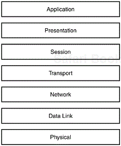
The top layer, Layer Seven, is the Application Layer and is where the end user actually interfaces with the computer itself. Layer Seven encompasses such applications as the web, telnet, SSH, and email.
Layer Six, the Presentation Layer, presents data to the Application Layer. Computers take generic data and turn it into formats such as text, images, sound, and video at this layer. Data translation, compression, and encryption are handled here.
Layer Five, the Session Layer, handles data by providing a means of transport for the Presentation Layer. Examples of applications that utilize the Session Layer include X Window, NFS, AppleTalk, and RPC.
The Transport Layer, Layer Four, provides error detection and control, multiplexing transport connections onto data connections (multiplexing allows the data from different applications to share one data stream), flow control, and transport to the Network Layer.
Layer Three, the Network Layer, is responsible for transmitting data across networks. Two types of packets are used at this level, including data packets and route updates. Routers that work on this level keep data about network addresses, routing tables, and the distance for remote networks.
Layer Two, the Data Link Layer, translates messages from the Network Layer into the Physical Layer. This layer handles error control, reliability, and integrity issues. The Network Layer adds frames to the data and adds a customized header containing the source and destination address. The layer identifies each device on the network as well.
The bottom layer, Layer One, or the Physical Layer, sends and receives information in the form of ones and zeros. The characteristics of this layer include specifications for signal voltages, wire width and length, and signaling.
Many devices operate at different levels. The hub, when cabled, only amplifies or retransmits data through all its ports. In this way, it operates only on Layer One. However, a switch operates on Layers One and Two, and a router operates on Layers One, Two, and Three. The end user’s workstation would typically handle Layers Five, Six, and Seven (although the versatility of Linux could allow it to handle much more).
The point of having such a layered approach is so that the different aspects of networking can work with each other—yet remain independent. This allows application developers the freedom to work on one aspect of a layer while expecting the other layers to work as planned. Without these layers, the developer would have to make sure that every aspect of the application included support for each layer. In other words, instead of just coding a simple game, the development team would not only have to code the game itself, but also the picture formats, the TCP/IP stack, and have to develop the router to transmit the information.
Why is learning this so important for clustering? First of all, it aids in troubleshooting. Knowing where the problem lies is the most important step to solving the problem. Every troubleshooting method needs to start somewhere, and by going over the OSI model, you can easily diagnose where the problem lies. By isolating each layer, you can track down problems and resolve them.
Different types of clusters need different types of network topologies depending on the framework involved. A HA network might need more attention to detail regarding security to maintain uptime than a distributed computing environment or a parallel clustering scenario.
Picture the following HA scenario, if you will, as shown in Figure 1.4. A nationwide bank has Points of Presence (POP) in three cities across the United States. Each city has its own cluster with its own database and each is connected directly to the Internet from its own city, but yet each city has to have access to the other’s data. How is this best achieved? Topologies have to be clearly thought about in advance. Consider the topology of clusters spread across a WAN, for instance.
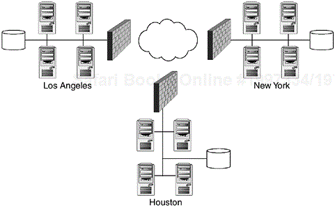
In this scenario, three sites are connected over the public Internet, with a firewall for security. This isn’t the most effective method of achieving high availability, but it’s a common scenario.
One way to go about redesigning this scenario is to remove two satellite cities from the Internet and connect each of these cities through direct frame relay to the internal network, thereby dropping the firewall from two of the satellite offices. Another approach would be to implement a load balanced network. POPs could easily be placed in key locations across the country so that customers could have relatively local access to the financial data. But because the data has to be synchronized between three cities in real time, the bandwidth involved would be tremendous.
A parallel cluster still needs a network design, although one that is much simpler in scope. Before fast ethernet to the desktop and gigabit ethernet for servers was the common standard, hypercubes were the primary means for designing high-performance clusters. A hypercube is a specific method to layout a parallel cluster, usually using regular ethernet. The trick to designing a hypercube was that each computer would have to have a direct network connection to each other node in the cube. This worked well with smaller cubes, although the size of the cube was somewhat limited due to the amount of network cards that could fit in any one computer. Larger clusters required meshed designs with hubs to support each node and the requisite multiple connections. Needless to say, they’re quite messy because of all the intermeshed cabling. With the advent of fast ethernet and gigabit ethernet, a simple managed or unmanaged switch will take care of most of the bandwidth problems. Of course, “the faster, the better” is the general motto, so be sure to consider the network when budgeting your cluster.
Along with the physical development of the cluster and the network topology, deciding which services to enable is the next step toward a finished clustering solution. Although most Linux distributions offer access to all the standard services listed in /etc/services, the system administrator has to determine if those services are applicable to their environment.
In a high-security environment, the system administrator might have no choice but to tighten down these resources. The most common ways of disabling services include restricting access to them through the firewall, by setting up an internal network, or by utilizing hosts:deny and hosts:allow. Those services that are accessible though inet can be commented out in /etc/inetd.conf.
It’s no surprise that, to enable web services, you have to keep access to port 80—and 443 if you’re going to enable web support over Secure Sockets Layer (SSL). In addition, what you also have to keep in mind when designing your cluster is access to the backup devices, whether or not to allow SSH, telnet, or ftp, and so on. In fact, it’s a good idea to totally disallow telnet across the environment and replace it with secure shell. Not only does this allow secure logins, but also secure ftp transfers for internal office use. FTP servers should still use regular ftp, of course, but only for dedicated servers.
After you decide which services to keep on the public network, it’s a wise idea to make a nonroutable network strictly for management purposes. This management network serves two purposes: One, it enables redundancy. The administrator has the ability to gain access to the box if the public network goes down or is totally saturated from public use. Secondly, it gives the opportunity for a dedicated backup network. The bandwidth from nightly backups each night has the potential to saturate a public network.
Realistically, you don’t want to keep your parallel cluster on a public network. A private network lessens the chance of compromised data and machines. Unless you keep your cluster so that anyone can run jobs on it, the added benefit of a nonroutable network greatly outweighs the potential risks.
Just as the state of computing has come a long way, so has clustering in general. As Linux matures, so does its ability to handle larger clusters using commodity hardware, as well as mission-critical data across HA clusters.
Clustering under Linux is similar to clusters under other operating systems, although it excels in its ability to run under many different commodity hardware configurations. With the right configuration, however, it can provide supercomputer-like performance at a fraction of the cost. The right configuration, of course, changes upon the needs of the organization and the cluster that is implemented.