Chapter 6
Programming in MATLAB
A computer program is a sequence of computer commands. In a simple program the commands are executed one after the other in the order they are typed. In this book, for example, all the programs that have been presented so far in script files are simple programs. Many situations, however, require more sophisticated programs in which commands are not necessarily executed in the order they are typed, or different commands (or groups of commands) are executed when the program runs with different input variables. For example, a computer program that calculates the cost of mailing a package uses different mathematical expressions to calculate the cost depending on the weight and size of the package, the content (books are less expensive to mail), and the type of service (airmail, ground, etc.). In other situations there might be a need to repeat a sequence of commands several times within a program. For example, programs that solve equations numerically repeat a sequence of calculations until the error in the answer is smaller than some measure.
MATLAB provides several tools that can be used to control the flow of a program. Conditional statements (Section 6.2) and the switch structure (Sections 6.3) make it possible to skip commands or to execute specific groups of commands in different situations. For loops and while loops (Sections 6.4) make it possible to repeat a sequence of commands several times.
It is obvious that changing the flow of a program requires some kind of decision-making process within the program. The computer must decide whether to execute the next command or to skip one or more commands and continue at a different line in the program. The program makes these decisions by comparing values of variables. This is done by using relational and logical operators, which are explained in Sections 6.1.
It should also be noted that user-defined functions (introduced in Chapter 7) can be used in programming. A user-defined function can be used as a subprogram. When the main program reaches the command line that has the user-defined function, it provides input to the function and “waits” for the results. The user defined function carries out the calculations and transfers the results back to the main program, which then continues to the next command.
6.1 RELATIONAL AND LOGICAL OPERATORS
A relational operator compares two numbers by determining whether a comparison statement (e.g., 5 < 8) is true or false. If the statement is true, it is assigned a value of 1. If the statement is false, it is assigned a value of 0. A logical operator examines true/false statements and produces a result that is true (1) or false (0) according to the specific operator. For example, the logical AND operator gives 1 only if both statements are true. Relational and logical operators can be used in mathematical expressions and, as will be shown in this chapter, are frequently used in combination with other commands to make decisions that control the flow of a computer program.
Relational operators:
Relational operators in MATLAB are:
| Relational operator | Description |
|---|---|
| < | Less than |
| > | Greater than |
| <= | Less than or equal to |
| >= | Greater than or equal to |
| == | Equal to |
| ~= | Not Equal to |
Note that the “equal to” relational operator consists of two = signs (with no space between them), since one = sign is the assignment operator. In other relational operators that consist of two characters, there also is no space between the characters (<=, >=, ~=).
• Relational operators are used as arithmetic operators within a mathematical expression. The result can be used in other mathematical operations, in addressing arrays, and together with other MATLAB commands (e.g., if) to control the flow of a program.
• When two numbers are compared, the result is 1 (logical true) if the comparison, according to the relational operator, is true, and 0 (logical false) if the comparison is false.
• If two scalars are compared, the result is a scalar 1 or 0. If two arrays are compared (only arrays of the same size can be compared), the comparison is done element-by-element, and the result is a logical array of the same size with 1s and 0s according to the outcome of the comparison at each address.
• If a scalar is compared with an array, the scalar is compared with every element of the array, and the result is a logical array with 1s and 0s according to the outcome of the comparison of each element.
Some examples are:

• The results of a relational operation with vectors, which are vectors with 0s and 1s, are called logical vectors and can be used for addressing vectors. When a logical vector is used for addressing another vector, it extracts from that vector the elements in the positions where the logical vector has 1s. For example:
aravinda
• Numerical vectors and arrays with the numbers 0s and 1s are not the same as logical vectors and arrays with 0s and 1s. Numerical vectors and arrays can not be used for addressing. Logical vectors and arrays, however, can be used in arithmetic operations. The first time a logical vector or an array is used in arithmetic operations it is changed to a numerical vector or array.
• Order of precedence: In a mathematical expression that includes relational and arithmetic operations, the arithmetic operations (+, −, *, /, ) have precedence over relational operations. The relational operators themselves have equal precedence and are evaluated from left to right. Parentheses can be used to alter the order of precedence. Examples are:

Logical operators in MATLAB are:

• Logical operators have numbers as operands. A nonzero number is true, and a zero number is false.
• Logical operators (like relational operators) are used as arithmetic operators within a mathematical expression. The result can be used in other mathematical operations, in addressing arrays, and together with other MATLAB commands (e.g., if) to control the flow of a program.
• Logical operators (like relational operators) can be used with scalars and arrays.
• The logical operations AND and OR can have both operands as scalars, both as arrays, or one as an array and one as a scalar. If both are scalars, the result is a scalar 0 or 1. If both are arrays, they must be of the same size and the logical operation is done element-by-element. The result is an array of the same size with 1s and 0s according to the outcome of the operation at each position. If one operand is a scalar and the other is an array, the logical operation is done between the scalar and each of the elements in the array and the outcome is an array of the same size with 1s and 0s.
• The logical operation NOT has one operand. When it is used with a scalar, the outcome is a scalar 0 or 1. When it is used with an array, the outcome is an array of the same size with 0s in positions where the array has nonzero numbers and 1s in positions where the array has 0s.
Following are some examples:
![]()

Order of precedence:
Arithmetic, relational, and logical operators can be combined in mathematical expressions. When an expression has such a combination, the result depends on the order in which the operations are carried out. The following is the order used by MATLAB:
| Precedence | Operation |
|---|---|
| 1 (highest) | Parentheses (if nested parentheses exist, inner ones have precedence) |
| 2 | Exponentiation |
| 3 | Logical NOT (~) |
| 4 | Multiplication, division |
| 5 | Addition, subtraction |
| 6 | Relational operators (>, <, >=, <=, = =, ~=) |
| 7 | Logical AND (&) |
| 8(lowest) | Logical OR (|) |
If two or more operations have the same precedence, the expression is executed in order from left to right.
It should be pointed out here that the order shown above is the one used since MATLAB 6. Previous versions of MATLAB used a slightly different order (& did not have precedence over |), so the user must be careful. Compatibility problems between different versions of MATLAB can be avoided by using parentheses even when they are not required.
The following are examples of expressions that include arithmetic, relational, and logical operators:

Built-in logical functions:
MATLAB has built-in functions that are equivalent to the logical operators. These functions are:
and(A,B) |
equivalent to A&B |
or(A,B) |
equivalent to A|B |
not(A) |
equivalent to ~A |
In addition, MATLAB has other logical built-in functions, some of which are described in the following table:

The operations of the four logical operators, and, or, xor, and not can be summarized in a truth table:

![]()
Sample Problem 6-1: Analysis of temperature data
The following were the daily maximum temperatures (in °F) in Washington, DC, during the month of April 2002: 58 73 73 53 50 48 56 73 73 66 69 63 74 82 84 91 93 89 91 80 59 69 56 64 63 66 64 74 63 69 (data from the U.S. National Oceanic and Atmospheric Administration). Use relational and logical operations to determine the following:
(a) The number of days the temperature was above 75°.
(b) The number of days the temperature was between 65° and 80°.
(c) The days of the month when the temperature was between 50° and 60°.
Solution
In the script file below the temperatures are entered in a vector. Relational and logical expressions are then used to analyze the data.

The script file (saved as Exp6_1) is executed in the Command Window:

![]()
6.2 CONDITIONAL STATEMENTS
A conditional statement is a command that allows MATLAB to make a decision of whether to execute a group of commands that follow the conditional statement, or to skip these commands. In a conditional statement, a conditional expression is stated. If the expression is true, a group of commands that follow the statement are executed. If the expression is false, the computer skips the group. The basic form of a conditional statement is:

• Conditional statements can be a part of a program written in a script file or a user-defined function (Chapter 7).
• As shown below, for every if statement there is an end statement.
The if statement is commonly used in three structures, if-end, if-else-end, and if-elseif-else-end, which are described next.
6.2.1 The if-end Structure
The if-end conditional statement is shown schematically in Figure 6-1. The figure shows how the commands are typed in the program, and a flowchart that symbolically shows the flow, or the sequence, in which the commands are executed. As the program executes, it reaches the if statement. If the conditional expression in the if statement is true (1), the program continues to execute the commands that follow the if statement all the way down to the end statement. If the conditional expression is false (0), the program skips the group of commands between the if and the end, and continues with the commands that follow the end.

Figure 6-1: The structure of the if-end conditional statement.
The words if and end appear on the screen in blue, and the commands between the if statement and the end statement are automatically indented (they don’t have to be), which makes the program easier to read. An example where the if-end statement is used in a script file is shown in Sample Problem 6-2.
![]()
Sample Problem 6-2: Calculating worker’s pay
A worker is paid according to his hourly wage up to 40 hours, and 50% more for overtime. Write a program in a script file that calculates the pay to a worker. The program asks the user to enter the number of hours and the hourly wage. The program then displays the pay.
Solution
The program in a script file is shown below. The program first calculates the pay by multiplying the number of hours by the hourly wage. Then an if statement checks whether the number of hours is greater than 40. If so, the next line is executed and the extra pay for the hours above 40 is added. If not, the program skips to the end.
t=input('Please enter the number of hours worked  ');

h=input('Please enter the hourly wage in $  ');

Pay=t*h;

if t>40

    Pay=Pay+(t-40)*0.5*h;

end

fprintf('The worker''s pay is  $ %5.2f',Pay)
Application of the program (in the Command Window) for two cases is shown below (the file was saved as Workerpay):
>> Workerpay

Please enter the number of hours worked  35

Please enter the hourly wage in $  8

The worker’s pay is  $ 280.00

>> Workerpay

Please enter the number of hours worked  50

Please enter the hourly wage in $  10

The worker’s pay is  $ 550.00
![]()
6.2.2 The if-else-end Structure
The if-else-end structure provides a means for choosing one group of commands, out of a possible two groups, for execution. The if-else-end structure is shown in Figure 6-2. The figure shows how the commands are typed in the program, and includes a flowchart that illustrates the flow, or the sequence, in

Figure 6-2: The structure of the if-else-end conditional statement.
which the commands are executed. The first line is an if statement with a conditional expression. If the conditional expression is true, the program executes group 1 of commands between the if and the else statements and then skips to the end. If the conditional expression is false, the program skips to the else and then executes group 2 of commands between the else and the end.
6.2.3 The if-elseif-else-end Structure
The if-elseif-else-end structure is shown in Figure 6-3. The figure shows how the commands are typed in the program, and gives a flowchart that illustrates the flow, or the sequence, in which the commands are executed. This structure includes two conditional statements (if and elseif) that make it possible to select one out of three groups of commands for execution. The first line is an if statement with a conditional expression. If the conditional expression is true, the program executes group 1 of commands between the if and the elseif statements and then skips to the end. If the conditional expression in the if statement is false, the program skips to the elseif statement. If the conditional expression in the elseif statement is true, the program executes group 2 of commands between the elseif and the else and then skips to the end. If the conditional expression in the elseif statement is false, the program skips to the else and executes group 3 of commands between the else and the end.

Figure 6-3: The structure of the if-elseif-else-end conditional statement.
It should be pointed out here that several elseif statements and associated groups of commands can be added. In this way more conditions can be included. Also, the else statement is optional. This means that in the case of several elseif statements and no else statement, if any of the conditional statements is true the associated commands are executed; otherwise nothing is executed.
The following example uses the if-elseif-else-end structure in a program.
![]()
Sample Problem 6-3: Water level in water tower
The tank in a water tower has the geometry shown in the figure (the lower part is a cylinder and the upper part is an inverted frustum of a cone). Inside the tank there is a float that indicates the level of the water. Write a MATLAB program that determines the volume of the water in the tank from the position (height h) of the float. The program asks the user to enter a value of h in m, and as output displays the volume of the water in m3.

Solution
For 0 ≤ h ≤ 19 m the volume of the water is given by the volume of a cylinder with height h: V = π12.52h.
For 19 < h ≤ 33 m the volume of the water is given by adding the volume of a cylinder with h = 19 m, and the volume of the water in the cone:
![]()
where ![]() .
.
The program is:
% The program calculates the volume of the water in the

water tower.

h=input('Please enter the height of the float in meter  ');

if h > 33

   disp('ERROR. The height cannot be larger than 33 m.')

elseif h < 0

   disp('ERROR. The height cannot be a negative number.')

elseif h <= 19

   v = pi*12.5^2*h;

   fprintf('The volume of the water is %7.3f cubic meter.
',v)

else

   rh=12.5+10.5*(h-19)/14;

   v=pi*12.5^2*19+pi*(h-19)*(12.5^2+12.5*rh+rh^2)/3;

   fprintf('The volume of the water is %7.3f cubic meter.
',v)

end
The following is the display in the Command Window when the program is used with three different values of water height.
Please enter the height of the float in meter  8

The volume of the water is 3926.991 cubic meter.

Please enter the height of the float in meter  25.7

The volume of the water is 14114.742 cubic meter.

Please enter the height of the float in meter  35

ERROR. The height cannot be larger than 33 m.
![]()
6.3 THE switch-case STATEMENT
The switch-case statement is another method that can be used to direct the flow of a program. It provides a means for choosing one group of commands for execution out of several possible groups. The structure of the statement is shown in Figure 6-4.
• The first line is the switch command, which has the form:
![]()
The switch expression can be a scalar or a string. Usually it is a variable that has an assigned scalar or a string. It can also be, however, a mathematical expression that includes pre-assigned variables and can be evaluated.
• Following the switch command are one or several case commands. Each has a value (can be a scalar or a string) next to it (value1, value2, etc.) and an associated group of commands below it.
• After the last case command there is an optional otherwise command followed by a group of commands.
• The last line must be an end statement.
How does the switch-case statement work?
The value of the switch expression in the switch command is compared with the values that are next to each of the case statements. If a match is found, the group of commands that follow the case statement with the match are executed. (Only one group of commands—the one between the case that matches and either the case, otherwise, or end statement that is next—is executed).
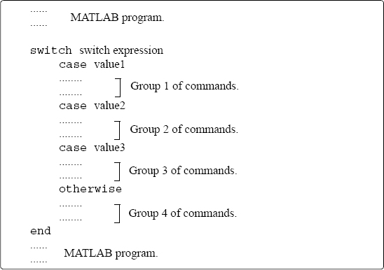
Figure 6-4: The structure of a switch-case statement.
• If there is more than one match, only the first matching case is executed.
• If no match is found and the otherwise statement (which is optional) is present, the group of commands between otherwise and end is executed.
• If no match is found and the otherwise statement is not present, none of the command groups is executed.
• A case statement can have more than one value. This is done by typing the values in the form: {value1, value2, value3, ...}. (This form, which is not covered in this book, is called a cell array.) The case is executed if at least one of the values matches the value of switch expression.
A Note: In MATLAB only the first matching case is executed. After the group of commands associated with the first matching case are executed, the program skips to the end statement. This is different from the C language, where break statements are required.
![]()
Sample Problem 6-4: Converting units of energy
Write a program in a script file that converts a quantity of energy (work) given in units of either joule, ft-lb, cal, or eV to the equivalent quantity in different units specified by the user. The program asks the user to enter the quantity of energy, its current units, and the desired new units. The output is the quantity of energy in the new units.
The conversion factors are: 0.738 ft-lb = 0.239 cal = 6.24 × 10¹⁸ eV. Use the program to:
(a) Convert 150 J to ft-lb.
(b) Convert 2,800 cal to J.
(c) Convert 2.7 eV to cal.
Solution
The program includes two sets of switch-case statements and one if-else-end statement. The first switch-case statement is used to convert the input quantity from its initial units to units of joules. The second is used to convert the quantity from joules to the specified new units. The if-else-end statement is used to generate an error message if units are entered incorrectly.


As an example, the script file (saved as EnergyConversion) is used next in the Command Window to make the conversion in part (b) of the problem statement.
>> EnergyConversion

Enter the value of the energy (work) to be converted: 2800

Enter the current units (J, ft-lb, cal, or eV):  cal

Enter the new units (J, ft-lb, cal, or eV):  J

E = 11715.5 J
![]()
6.4 LOOPS
A loop is another method to alter the flow of a computer program. In a loop, the execution of a command, or a group of commands, is repeated several times consecutively. Each round of execution is called a pass. In each pass at least one variable, but usually more than one, or even all the variables that are defined within the loop, are assigned new values. MATLAB has two kinds of loops. In for-end loops (Sections 6.4.1) the number of passes is specified when the loop starts. In while-end loops (Sections 6.4.2) the number of passes is not known ahead of time, and the looping process continues until a specified condition is satisfied. Both kinds of loops can be terminated at any time with the break command (see Sections 6.6).
6.4.1 for-end Loops
In for-end loops the execution of a command, or a group of commands, is repeated a predetermined number of times. The form of a loop is shown in Figure 6-5.
• The loop index variable can have any variable name (usually i, j, k, m, and n are used, but i and j should not be used if MATLAB is used with complex numbers).

Figure 6-5: The structure of a for-end loop.
• In the first pass k = f and the computer executes the commands between the for and end commands. Then, the program goes back to the for command for the second pass. k obtains a new value equal to k = f + s, and the commands between the for and end commands are executed with the new value of k. The process repeats itself until the last pass, where k = t. Then the program does not go back to the for, but continues with the commands that follow the end command. For example, if k = 1:2:9, there are five loops, and the corresponding values of k are 1, 3, 5, 7, and 9.
• The increment s can be negative (i.e.; k = 25:–5:10 produces four passes with k = 25, 20, 15, 10).
• If the increment value s is omitted, the value is 1 (default) (i.e.; k = 3:7 produces five passes with k = 3, 4, 5, 6, 7).
• If f = t, the loop is executed once.
• If f > t and s > 0, or if f < t and s < 0, the loop is not executed.
• If the values of k, s, and t are such that k cannot be equal to t, then if s is positive, the last pass is the one where k has the largest value that is smaller than t (i.e., k = 8:10:50 produces five passes with k = 8, 18, 28, 38, 48). If s is negative, the last pass is the one where k has the smallest value that is larger than t.
• In the for command k can also be assigned a specific value (typed as a vector). Example: for k = [7 9 –1 3 3 5].
• The value of k should not be redefined within the loop.
• Each for command in a program must have an end command.
• The value of the loop index variable (k) is not displayed automatically. It is possible to display the value in each pass (which is sometimes useful for debugging) by typing k as one of the commands in the loop.
• When the loop ends, the loop index variable (k) has the value that was last assigned to it.
A simple example of a for-end loop (in a script file) is:
for k=1:3:10

     x = k^2

end
When this program is executed, the loop is executed four times. The value of k in the four passes is k = 1, 4, 7, and 10, which means that the values that are assigned to x in the passes are x = 1, 16, 49, and 100, respectively. Since a semicolon is not typed at the end of the second line, the value of x is displayed in the Command Window at each pass. When the script file is executed, the display in the Command Window is:
>> x =

     1

x =

    16

x =

    49

x =

   100
![]()
Sample Problem 6-5: Sum of a series
(a) Use a for-end loop in a script file to calculate the sum of the first n terms of the series:![]() . Execute the script file for n = 4 and n = 20.
. Execute the script file for n = 4 and n = 20.
(b) The function sin(x) can be written as a Taylor series by:
![]()
Write a user-defined function file that calculates sin(x) by using the Taylor series. For the function name and arguments use y = Tsin(x,n). The input arguments are the angle x in degrees and n the number of terms in the series. Use the function to calculate sin(150°) using three and seven terms.
Solution
(a) A script file that calculates the sum of the first n terms of the series is shown below.
The summation is done with a loop. In each pass one term of the series is calculated (in the first pass the first term, in the second pass the second term, and so on) and is added to the sum of the previous elements. The file is saved as Exp6_5a and then executed twice in the Command Window:

>> Exp6_5a

Enter the number of terms 4

The sum of the series is: -0.125000

>> Exp7_5a

Enter the number of terms 20

The sum of the series is: -0.222216
(b) A user-defined function file that calculates sin(x) by adding n terms of a Taylor series is shown below.

The first element corresponds to k = 0, which means that in order to add n terms of the series, in the last loop k = n – 1. The function is used in the Command Window to calculate sin(150°) using three and seven terms:


A note about for-end loops and element-by-element operations:
In some situations the same end result can be obtained by either using for-end loops or using element-by-element operations. Sample Problem 6-5 illustrates how the for-end loop works, but the problem can also be solved by using element-by-element operations (see Problems 7 and 8 in Section 3.9). Element-by-element operations with arrays are one of the superior features of MATLAB that provide the means for computing in circumstances that otherwise require loops. In general, element-by-element operations are faster than loops and are recommended when either method can be used.
![]()
Sample Problem 6-6: Modify vector elements
A vector is given by V = [5, 17, –3, 8, 0, –7, 12, 15, 20, –6, 6, 4, –7, 16]. Write a program as a script file that doubles the elements that are positive and are divisible by 3 or 5, and, raises to the power of 3 the elements that are negative but greater than –5.
Solution
The problem is solved by using a for-end loop that has an if-elseif-end conditional statement inside. The number of passes is equal to the number of elements in the vector. In each pass one element is checked by the conditional statement. The element is changed if it satisfies the conditions in the problem statement. A program in a script file that carries out the required operations is:

The file is saved as Exp7_6 and then executed in the Command Window:
>> Exp7_6

V =

   10  17  -27  8  0  -7  24  30  40  -6  12  4

-8  16
![]()
6.4.2 while-end Loops
while-end loops are used in situations when looping is needed but the number of passes is not known in advance. In while-end loops the number of passes is not specified when the looping process starts. Instead, the looping process continues until a stated condition is satisfied. The structure of a while-end loop is shown in Figure 6-6.

Figure 6-6: The structure of a while-end loop.
The first line is a while statement that includes a conditional expression. When the program reaches this line the conditional expression is checked. If it is false (0), MATLAB skips to the end statement and continues with the program. If the conditional expression is true (1), MATLAB executes the group of commands that follow between the while and end commands. Then MATLAB jumps back to the while command and checks the conditional expression. This looping process continues until the conditional expression is false.
For a while-end loop to execute properly:
• The conditional expression in the while command must include at least one variable.
• The variables in the conditional expression must have assigned values when MATLAB executes the while command for the first time.
• At least one of the variables in the conditional expression must be assigned a new value in the commands that are between the while and the end. Otherwise, once the looping starts it will never stop, since the conditional expression will remain true.
An example of a simple while-end loop is shown in the following program. In this program a variable x with an initial value of 1 is doubled in each pass as long as its value is equal to or smaller than 15.

When this program is executed the display in the Command Window is:

Important note:
When writing a while-end loop, the programmer has to be sure that the variable (or variables) that are in the conditional expression and are assigned new values during the looping process will eventually be assigned values that make the conditional expression in the while command false. Otherwise the looping will continue indefinitely (indefinite loop). In the example above if the conditional expression is changed to x >= 0.5, the looping will continue indefinitely. Such a situation can be avoided by counting the passes and stopping the looping if the number of passes exceeds some large value. This can be done by adding the maximum number of passes to the conditional expression, or by using the break command (Sections 6.6).
Since no one is free from making mistakes, a situation of indefinite looping can occur in spite of careful programming. If this happens, the user can stop the execution of an indefinite loop by pressing the Ctrl + C or Ctrl + Break keys.
![]()
Sample Problem 6-7: Taylor series representation of a function
The function f(x) = ex can be represented in a Taylor series by ![]() . Write a program in a script file that determines ex by using the Taylor series representation. The program calculates ex by adding terms of the series and stopping when the absolute value of the term that was added last is smaller than 0.0001. Use a
. Write a program in a script file that determines ex by using the Taylor series representation. The program calculates ex by adding terms of the series and stopping when the absolute value of the term that was added last is smaller than 0.0001. Use a while-end loop, but limit the number of passes to 30. If in the 30th pass the value of the term that is added is not smaller than 0.0001, the program stops and displays a message that more than 30 terms are needed.
Use the program to calculate e2, e−4, and e21.
Solution
The first few terms of the Taylor series are:
![]()
A program that uses the series to calculate the function is shown next. The program asks the user to enter the value of x. Then the first term, an, is assigned the number 1, and an is assigned to the sum S. Then, from the second term on, the program uses a while loop to calculate the nth term of the series and add it to the sum. The program also counts the number of terms n. The conditional expression in the while command is true as long as the absolute value of the nth an term is larger than 0.0001, and the number of passes n is smaller than 30. This means that if the 30th term is not smaller than 0.0001, the looping stops.

The program uses an if-else-end statement to display the results. If the looping stopped because the 30th term is not smaller than 0.0001, it displays a message indicating this. If the value of the function is calculated successfully, it displays the value of the function and the number of terms used. When the program executes, the number of passes depends on the value of x. The program (saved as expox) is used to calculate e2 e−4, and e21:
>> expox

![]()
6.5 NESTED LOOPS AND NESTED CONDITIONAL STATEMENTS
Loops and conditional statements can be nested within other loops or conditional statements. This means that a loop and/or a conditional statement can start (and end) within another loop or conditional statement. There is no limit to the number of loops and conditional statements that can be nested. It must be remembered, however, that each if, case, for, and while statement must have a corresponding end statement. Figure 6-7 shows the structure of a nested for-end loop within another for-end loop. In the loops shown in this figure, if, for example, n = 3 and m = 4, then first k = 1 and the nested loop executes four times with h = 1, 2, 3, 4. Next k = 2 and the nested loop executes again four times with h = 1, 2, 3, 4. Finally k = 3 and the nested loop executes again four times. Every time a nested loop is typed, MATLAB automatically indents the new loop relative to the outside loop. Nested loops and conditional statements are demonstrated in the following sample problem.

Figure 6-7: Structure of nested loops.
![]()
Sample Problem 6-8: Creating a matrix with a loop
Write a program in a script file that creates an n × m matrix with elements that have the following values. The value of each element in the first row is the number of the column. The value of each element in the first column is the number of the row. The rest of the elements each has a value equal to the sum of the element above it and the element to the left. When executed, the program asks the user to enter values for n and m.
Solution
The program, shown below, has two loops (one nested) and a nested ifelseif-else-end structure. The elements in the matrix are assigned values row by row. The loop index variable of the first loop, k, is the address of the row, and the loop index variable of the second loop, h, is the address of the column.

The program is executed in the Command Window to create a 4 × 5 matrix.
>> Chap6_exp8

Enter the number of rows 4

Enter the number of columns 5

A =

      1     2     3     4     5

      2     4     7    11    16

      3     7    14    25    41

      4    11    25    50    91
![]()
6.6 THE break AND continue COMMANDS
The break command:
• When inside a loop (for or while), the break command terminates the execution of the loop (the whole loop, not just the last pass). When the break command appears in a loop, MATLAB jumps to the end command of the loop and continues with the next command (it does not go back to the for command of that loop).
• If the break command is inside a nested loop, only the nested loop is terminated.
• When a break command appears outside a loop in a script or function file, it terminates the execution of the file.
• The break command is usually used within a conditional statement. In loops it provides a method to terminate the looping process if some condition is met —for example, if the number of loops exceeds a predetermined value, or an error in some numerical procedure is smaller than a predetermined value. When typed outside a loop, the break command provides a means to terminate the execution of a file, such as when data transferred into a function file is not consistent with what is expected.
The continue command:
• The continue command can be used inside a loop (for or while) to stop the present pass and start the next pass in the looping process.
• The continue command is usually a part of a conditional statement. When MATLAB reaches the continue command, it does not execute the remaining commands in the loop, but skips to the end command of the loop and then starts a new pass.
6.7 EXAMPLES OF MATLAB APPLICATIONS
![]()
Sample Problem 6-9: Withdrawing from a retirement account.
A person in retirement is depositing $300,000 in a saving account that pays 5% interest per year. The person plans to withdraw money from the account once a year. He starts by withdrawing $25,000 after the first year, and in future years he increases the amount he withdraws according to the inflation rate. For example, if the inflation rate is 3%, he withdraws $25,750 after the second year. Calculate the number of years the money in the account will last assuming a constant yearly inflation rate of 2%. Make a plot that shows the yearly withdrawals and the balance of the account over the years.
Solution
The problem is solved by using a loop (a while loop since the number of passes is not known before the loop starts). In each pass the amount to be withdrawn and the account balance are calculated. The looping continues as long as the account balance is larger than or equal to the amount to be withdrawn. The following is a program in a script file that solves the problem. In the program, year is a vector in which each element is a year number, W is a vector with the amount withdrawn each year, and AB is a vector with the account balance each year.

The program is executed in the following Command Window:
>> Chap6_exp9

The money will last for 15 years.
The program also generates the following figure (axis labels and legend were added to the plot by using the Plot Editor).

![]()
Sample Problem 6-10: Creating a random list
Six singers—John, Mary, Tracy, Mike, Katie, and David—are performing in a competition. Write a MATLAB program that generates a list of a random order in which the singers will perform.
Solution
An integer (1 through 6) is assigned to each name (1 to John, 2 to Mary, 3 to Tracy, 4 to Mike, 5 to Katie, and 6 to David). The program, shown below, first creates a list of the integers 1 through 6 in a random order. The integers are made the elements of six-element vector. This is done by using MATLAB’s built-in function randi (see Section 3.7) for assigning integers to the elements of the vector. To make sure that all the integers of the elements are different from each other, the integers are assigned one by one. Each integer that is suggested by the randi function is compared with all the integers that have been assigned to previous elements. If a match is found, the integer is not assigned, and randi is used for suggesting a new integer. Since each singer name is associated with an integer, once the integer list is complete the switch-case statement is used to create the corresponding name list.
clear, clc

n=6;

The while loop checks that every new integer (element) that is to be added to the vector L is not equal any of the integers in elements already in the vector L. If a match is found, it keeps generating new integers until the new integer is different from all the integers that are already in x.
When the program is executed, the following is displayed in the Command Window. Obviously, a list in a different order will be displayed every time the program is executed.
The performing order is:

Katie

Tracy

David

Mary

John

Mike
![]()
Sample Problem 6-11: Flight of a model rocket
The flight of a model rocket can be modeled as follows. During the first 0.15s the rocket is propelled upward by the rocket engine with a force of 16 N. The rocket then flies up while slowing down under the force of gravity. After it reaches the apex, the rocket starts to fall back down. When its downward velocity reaches 20 m/s, a parachute opens (assumed to open instantly), and the rocket continues to drop at a constant speed of 20 m/s until it hits the ground. Write a program that calculates and plots the speed and altitude of the rocket as a function of time during the flight.

Solution
The rocket is assumed to be a particle that moves along a straight line in the vertical plane. For motion with constant acceleration along a straight line, the velocity and position as a function of time are given by:
![]()
where v0 and s0 are the initial velocity and position, respectively. In the computer program the flight of the rocket is divided into three segments. Each segment is calculated in a while loop. In every pass the time increases by an increment.
Segment 1: The first 0.15s when the rocket engine is on. During this period, the rocket moves up with a constant acceleration. The acceleration is determined by drawing a free body and a mass acceleration diagram (shown on the right). From Newton’s second law, the sum of the forces in the vertical direction is equal to the mass times the acceleration (equilibrium equation):

![]()
Solving the equation for the acceleration gives:
![]()
The velocity and height as a function of time are:
![]()
where the initial velocity and initial position are both zero. In the computer program this segment starts at t = 0, and the looping continues as long as t < 0.15 s. The time, velocity, and height at the end of this segment are t1, v1, and h1.
Segment 2: The motion from when the engine stops until the parachute opens. In this segment the rocket moves with a constant deceleration g. The speed and height of the rocket as functions of time are given by:
![]()
In this segment the looping continues until the velocity of the rocket is –20 m/s (negative since the rocket moves down). The time and height at the end of this segment are t2 and h2.
Segment 3: The motion from when the parachute opens until the rocket hits the ground. In this segment the rocket moves with constant velocity (zero acceleration). The height as a function of time is given by h(t) = h2 − vchute(t−t2), where vchute is the constant velocity after the parachute opens. In this segment the looping continues as long as the height is greater than zero.
A program in a script file that carries out the calculations is shown below.


The accuracy of the results depends on the magnitude of the time increment Dt. An increment of 0.01 s appears to give good results. The conditional expression in the while commands also includes a condition for n (if n is larger than 50,000 the loop stops). This is done as a precaution to avoid an infinite loop in case there is an error in an of the statements inside the loop. The plots generated by the program are shown below (axis labels and text were added to the plots using the Plot Editor).

Note: The problem can be solved and programmed in different ways. The solution shown here is one option. For example, instead of using while loops, the times when the parachute opens and when the rocket hits the ground can be calculated first, and then for-end loops can be used instead of the while loop. If the times are determined first, it is possible also to use element-by-element calculations instead of loops.
![]()
Sample Problem 6-12: AC to DC converter
A half-wave diode rectifier is an electrical circuit that converts AC voltage to DC voltage. A rectifier circuit that consists of an AC voltage source, a diode, a capacitor, and a load (resistor) is shown in the figure. The voltage of the source is vs = v0 sin(ωt), where ω = 2πf, in which f is the frequency. The operation of the circuit is illustrated in the lower diagram where the dashed line shows the source voltage and the solid line shows the voltage across the resistor. In the first cycle, the diode is on (conducting current) from t = 0 until t = tA. At this time the diode turns off and the power to the resistor is supplied by the discharging capacitor t = tB. At the diode turns on again and continues to conduct current until t = tD. The cycle continues as long as the voltage source is on. In this simplified analysis of this circuit, the diode is assumed to be ideal and the capacitor is assumed to have no charge initially (at t = 0). When the diode is on, the resistor’s voltage and current are given by:
vR = v0 sin(ωt) and iR = v0 sin (ωt)/R

The current in the capacitor is:
iC = ωCv0 cos(ωt)
When the diode is off, the voltage across the resistor is given by:
vR = v0 sin(ωtA)e (−(t−tA))/(RC)
The times when the diode switches off (tA, tD, and so on) are calculated from the condition iR = −iC. The diode switches on again when the voltage of the source reaches the voltage across the resistor (time tB in the figure).
Write a MATLAB program that plots the voltage across the resistor vR and the voltage of the source vs as a function of time for 0 ≤ t ≤70 ms. The resistance of the load is 1,800 Ω, the voltage source V0 = 12 V, and f = 60 Hz. To examine the effect of capacitor size on the voltage across the load, execute the program twice, once with C = 45 μF and once with C = 10 μF.
A program that solves the problem is presented below. The program has two parts—one that calculates the voltage vR when the diode is on, and the other when the diode is off. The switch command is used for switching between the two parts. The calculations start with the diode on (the variable state=‘on’), and when iR − iC ≤ 0 the value of state is changed to ‘off’, and the program switches to the commands that calculate vR for this state. These calculations continue until vs ≥ vR, when the program switches back to the equations that are valid when the diode is on.

The two plots generated by the program are shown below. One plot shows the result with C = 45 μF and the other with C = 10 μF. It can be observed that with a larger capacitor the DC voltage is smoother (smaller ripple in the wave).

![]()
6.8 PROBLEMS
1. Evaluate the following expressions without using MATLAB. Check the answers with MATLAB.
(a) 12 − 4 < 5 × 3
(b) y = 8/4 > 6 × 3 − 42 > −3
(c) y = −3 <(8 − 12)+2 × (5 > 18/6 −4)2
(d) (~5+~0) × 6==3+3 ×~0
2. Given: a = −2, b = 3, c = 5. Evaluate the following expressions without using MATLAB. Check the answers with MATLAB.
(a) y = a − b > a − c < b
(b) y = −4 < a <0
(c) y = a − c < = b > a + c
(d) y = 3 × (c+a~=a/b-b)==(a+c)~=b
3. Given: v = [4 −1 2 3 1 −2 5 0] and μ = [5 –1 0 3 –3 2 1 5]. Evaluate the following expressions without using MATLAB. Check the answers with MATLAB.
(a) ~ ~u
(b) v = = ~u
(c) u = = abs(v)
(d) v >= u + v
4. Use the vectors v and u from Problem 3. Use relational operators to create a vector w that is made up of the elements of u that are smaller than or equal to the elements of v.
5. Evaluate the following expressions without using MATLAB. Check the answers with MATLAB.
(a) –3&3
(b) ~5<4&~0>–3
(c) –2&2>3|8/3
(d) –3<–1<~0|5<4<3
6. Use loops to create a 3×5 matrix in which the value of each element is its row number to the power of its column number divided by the sum of its row number and column number. For example, the value of element (2,3) is 23/(2+3) = 1.6.
7. A symmetric (5×5) Pascal matrix is displayed on the right. Write a MATLAB program that creates an n×n symmetric Pascal matrix. Use the program to create 4×4 and 7×7 Pascal matrices.

8. The average monthly precipitation (in.) for Boston and Seattle during 2012 are given in the vectors below (data from the U.S. National Oceanic and Atmospheric Administration). BOS = [2.67 1.00 1.21 3.09 3.43 4.71 3.88 3.08 4.10 2.62 1.01 5.93] SEA = [6.83 3.63 7.20 2.68 2.05 2.96 1.04 0.00 0.03 6.71 8.28 6.85] where the elements in the vectors are in the order of the months (January, February, etc.) Write a program in a script file to answer the following:
(a) Calculate the total precipitation for the year and monthly average precipitation in each city.
(b) How many months was the precipitation above the average in each city?
(c) How many months, and on which months, was the precipitation in Boston lower than the precipitation in Seattle?
9. Write a program in a script file that finds the smallest even integer that is divisible by 13 and by 16 whose square root is greater than 120. Use a loop in the program. The loop should start from 1 and stop when the number is found. The program prints the message “The required number is:” and then prints the number.
10. Fibonacci numbers are the numbers in a sequence in which the first two elements are 0 and 1, and the value of each subsequent element is the sum of the previous two elements:
0, 1, 1, 2, 3, 5, 8, 13, ...
Write a MATLAB program in a script file that determines and displays the first 20 Fibonacci numbers.
11. The reciprocal Fibonacci constant ![]() is defined by the infinite sum:
is defined by the infinite sum:
![]()
where Fn are the Fibonacci numbers 1, 1, 2, 3, 5, 8, 13, ... . Each element in this sequence of numbers is the sum of the previous two. Start by setting the first two elements equal to 1, then. Write a MATLAB program in a script file that calculates ![]() for a given n. Execute the program for n = 10, 50, and 100.
for a given n. Execute the program for n = 10, 50, and 100.
12. Write a program in a script file that determines the real roots of a quadratic equation ax2+bx+c = 0. Name the file quadroots. When the file runs, it asks the user to enter the values of the constants a, b, and c. To calculate the roots of the equation the program calculates the discriminant D, given by:
D = b2 − 4ac
If D > 0, the program displays message “The equation has two roots,” and the roots are displayed in the next line.
If D = 0, the program displays message “The equation has one root,” and the root is displayed in the next line.
If D < 0, the program displays message “The equation has no real roots.” Run the script file in the Command Window three times to obtain solutions to the following three equations:
(a) 3x2 + 6x + 3 = 0
(b) −3x2 + 4x−6 = 0
(c) −3x2 + 7x + 5 = 0
13. The value of π can be estimated by:

Write a program (using a loop) that determines the expression. Run the program with n = 100, n = 10000, and n = 1000000. Compare the result with pi. (Use format long.)
14. The value of π can be estimated from the expression:
![]()
Write a MATLAB program in a script file that determine π for any number of terms. The program asks the user to enter the number of terms, and then calculates the corresponding value of π. Execute the program with 5, 10, and 40 terms. Compare the result with pi. (Use format long.)
15. Write a program that generates a vector with 20 random elements between –10 and 10 and then finds the sum of the positive elements.
16. Write a program that (a) generates a vector with 20 random integer elements with integers between –10 and 10, (b) replaces all the negative integers with random integers between –10 and 10, (c) repeats (b) until all the elements are positive. The program should also count how many times (b) is repeated before all the elements are positive. When done, the program displays the vector and a statement that states how many iterations were needed for generating the vector.
17. Write a program that asks the user to input a vector of integers of arbitrary length. The program then counts the number of elements, the number of positive elements, and the number of negative elements divisible by 3. The program displays the vector that was entered and the results in sentence form, i.e. “The vector has XX elements. XX elements are positive and XX elements are negative divisible by 3”, where XX stands for the corresponding number of elements. Execute the program and when the program ask the user to input a vector type randi([-20 20],1,16). This creates a 16-element vector with random integers between –20 and 20.
18. A vector is given by x = [4.5 5 –16.12 21.8 10.1 10 –16.11 5 14 –3 3 2]. Using conditional statements and loops, write a program that rearranges the elements of x in order from the smallest to the largest. Do not use MATLAB’s built-in function sort.
19. The Pythagorean theorem states that a2 + b2 = c2. Write a MATLAB program in a script file that finds all the combinations of triples a, b, and c that are positive integers all smaller or equal to 50 that satisfy the Pythagorean theorem. Display the results in a three-column table in which every row corresponds to one triple. The first three rows of the table are:
3 4 5
5 12 13
6 8 10
20. A twin primes is a pair of prime numbers such that the difference between them is 2 (for example, 17 and 19). Write a computer program that finds all the twin primes between 10 and 500. The program displays the results in a two-column matrix in which each row is a twin prime. Do not use MATLAB’s built-in function isprime.
21. An isolated prime is a prime number p such that neither p − 2 nor p + 2 is prime. For example, 47 is an isolated prime since 45 and 49 are both not primes. Write a computer program that finds all the isolated primes between 50 and 100. Do not use MATLAB’s built-in function isprime.
22. A list of 30 exam scores is: 31, 70, 92, 5, 47, 88, 81, 73, 51, 76, 80, 90, 55, 23, 43, 98, 36, 87, 22, 61, 19, 69, 26, 82, 89, 99, 71, 59, 49, 64
Write a computer program that determines how many grades are between 0 and 19, between 20 and 39, between 40 and 59, between 60 and 79, and between 80 and 100. The results are displayed in the following form:
Grades between 0 and 19 2 students
Grades between 20 and 39 4 students
Grades between 40 and 59 6 students
and so on. (Hint: use the command fprintf to display the results.)
23. The Taylor series expansion for cos(x) is:
![]()
where x is in radians. Write a MATLAB program that determines cos(x) using the Taylor series expansion. The program asks the user to type a value for an angle in degrees. Then the program uses a loop for adding the terms of the Taylor series. If is the nth term in the series, then the sum Sn of the n terms is Sn = Sn−1 + an. In each pass calculate the estimated error E given by ![]() . Stop adding terms when E ≤0.000001. The program displays the value of cos(x). Use the program for calculating:
. Stop adding terms when E ≤0.000001. The program displays the value of cos(x). Use the program for calculating:
(a) cos(35°)
(b) sin(125°)
Compare the values with those obtained by using a calculator.
24. Write a MATLAB program in a script file that finds a positive integer n such that the sum of all the integers 1 + 2 + 3 +…+ n is a number between 100 and 1000 whose three digits are identical. As output, the program displays the integer n and the corresponding sum.
25. The following are formulas for calculating the training heart rate (THR) for men and women:
For men (Karvonen formula): THR = [(220 − AGE)− RHR] × INTEN + RHR
For women: THR = [(206 − 0.88 × AGE) − RHR] × INTEN + RHR
where AGE is the person’s age, RHR the resting heart rate, and INTEN the fitness level (0.55 for low, 0.65 for medium, and 0.8 for high fitness). Write a program in a script file that determines the THR. The program asks users to enter their gender (male or female), age (number), resting heart rate (number), and fitness level (low, medium, or high). The program then displays the training heart rate. Use the program for determining the training heart rate for the following two individuals:
(a) A 21-year-old male, resting heart rate of 62, and low fitness level.
(b) A 19-year-old female, resting heart rate of 67, and high fitness level.
26. Body Mass Index (BMI) is a measure of obesity. In standard units, it is calculated by the formula
![]()
where W is weight in pounds, and H is height in inches. The obesity classification is:

Write a program in a script file that calculates the BMI of a person. The program asks the person to enter his or her weight (lb) and height (in.). The program displays the result in a sentence that reads: “Your BMI value is XXX, which classifies you as SSSS,” where XXX is the BMI value rounded to the nearest tenth, and SSSS is the corresponding classification. Use the program for determining the obesity of the following two individuals:
(a) A person 6 ft 2 in. tall with a weight of 180 lb.
(b) A person 5 ft 1 in. tall with a weight of 150 lb.
27. Write a program in a script file that calculates the cost of shipping a package according to the following price schedule:

The program asks the user to enter the type of service (Ground, Express, or Overnight) and the weight of the package (two numbers. First for number of pounds and second for number of ounces.) The program then displays the cost for the shipment. Run the program three times for the following cases:
(a) Ground 2 lb 7 oz.
(b) Express 0 lb 7 oz.
(c) Overnight 5 lb 10 oz.
28. Write a program that determines the change given back to a customer in a self-service checkout machine of a supermarket for purchases of up to $50. The program generates a random number between 0.01 and 50.00 and displays the number as the amount to be paid. The program then asks the user to enter payment, which can be one $1 bill, one $5 bill, one $10 bill, one $20 bill, or one $50 bill. If the payment is less than the amount to be paid, an error message is displayed. If the payment is sufficient, the program calculates the change and lists the bills and/or the coins that make up the change, which has to be composed of the least number each of bills and coins. For example, if the amount to be paid is $2.33 and a $10 bill is entered as payment, then the change is one $5 bill, two $1 bills, two quarters, one dime, one nickel, and two pennies. Execute the program three times.
29. The concentration of a drug in the body Cp can be modeled by the equation:
![]()
where DG is the dosage administered (mg), Vd is the volume of distribution (L), Ka is the absorption rate constant (h–1), ke is the elimination rate constant (h–1), and t is the time (h) since the drug was administered. For a certain drug, the following quantities are given: DG = 150 mg, Vd = 50L, ka = 1.6 h−1, and ke = 0.4.h−1.
(a) A single dose is administered at t = 0. Calculate and plot CP versus t for 10 hours.
(b) A first dose is administered at t = 0, and subsequently four more doses are administered at intervals of 4 hours (i.e., at t = 4, 8, 12, 16). Calculate and plot CP versus t for 24 hours.
30. One numerical method for calculating the cubic root of a number, ![]() is in iterations. The process starts by choosing a value x1 as a first estimate of the solution. Using this value, a second, more accurate value x2 can be calculated with
is in iterations. The process starts by choosing a value x1 as a first estimate of the solution. Using this value, a second, more accurate value x2 can be calculated with ![]() , which is then used for calculating a third, still more accurate value x3, and so on. The general equation for calculating the value of xi + 1 from the value of xi is
, which is then used for calculating a third, still more accurate value x3, and so on. The general equation for calculating the value of xi + 1 from the value of xi is ![]() . Write a MATLAB program that calculates the cubic root of a number. In the program use x1 = P for the first estimate of the solution. Then, by using the general equation in a loop, calculate new, more accurate values. Stop the looping when the estimated relative error E defined by
. Write a MATLAB program that calculates the cubic root of a number. In the program use x1 = P for the first estimate of the solution. Then, by using the general equation in a loop, calculate new, more accurate values. Stop the looping when the estimated relative error E defined by ![]() is smaller than 0.00001. Use the program to calculate:
is smaller than 0.00001. Use the program to calculate:
![]()
31. Write a program in a script file that converts a measure of pressure given in units of either Pa, psi, atm, or torr to the equivalent quantity in different units specified by the user. The program asks the user to enter the amount of pressure, its current units, and the desired new units. The output is the specification of pressure in the new units. Use the program to:
(a) Convert 70 psi to Pa.
(b) Convert 120 torr to atm.
(c) Convert 8000 Pa to psi.
32. In a one-dimensional random walk, the position x of a walker is computed by:
xj = xj + s
where s is a random number. Write a program that calculates the number of steps required for the walker to reach a boundary x = ±B. Use MATLAB’s built-in function randn(1,1) to calculate s. Run the program 100 times (by using a loop) and calculate the average number of steps when B = 10.
33. The Sierpinski triangle can be implemented in MATLAB by plotting points iteratively according to one of the following three rules that are selected randomly with equal probability.

Write a program in a script file that calculates the x and y vectors and then plots y versus x as individual points (use plot(x,y,'^')). Start with x1 = 0 and y1 = 0. Run the program four times with 10, 100, 1,000, and 10,000 iterations.
34. Cam is a mechanical device that transforms rotary motion into linear motion. The shape of the disc is designed to produce a specified displacement profile. A displacement profile is a plot of the displacement of the follower as a function of the angle of rotation of the cam. The motion of a certain cam is given by the following equations:
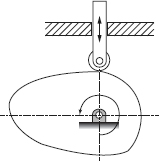

Write a MATLAB program that plots the displacement profile for one revolution. First create a 100 element vector for θ, then by using a loop and conditional statements calculate the value of y for the corresponding values of θ. Once y and θ are known, plot y vs. θ.
35. The overall grade in a course is determined from the grades of 6 quizzes, 3 midterms, and a final exam, using the following scheme:
Quizzes: Quizzes are graded on a scale from 0 to 10. The grade of the lowest quiz is dropped and the average of the 5 quizzes with the higher grades constitutes 30% of the course grade.
Midterms and final exam: Midterms and final exams are graded on a scale from 0 to 100. If the average of the midterm scores is higher than the score on the final exam, the average of the midterms constitutes 50% of the course grade and the grade of the final exam constitutes 20% of the course grade. If the final grade is higher than the average of the midterms, the average of the midterms constitutes 20% of the course grade and the grade of the final exam constitutes 50% of the course grade.
Write a computer program in a script file that determines the course grade for a student. The program first asks the user to enter the six quiz grades (in a vector), the three midterm grades (in a vector), and the grade of the final. Then the program calculates a numerical course grade (a number between 0 and 100). Finally, the program assigns a letter grade according to the following key: A for Grade ≥ 90, B for 80 ≤ Grade < 90, C for 70 ≤ Grade < 80, D for 60 ≤ Grade < 70, and E for a grade lower than 60. Execute the program for the following cases:
(a) Quiz grades: 6, 10, 6, 8, 7, 8. Midterm grades: 82, 95, 89. Final exam: 81.
(b) Quiz grades: 9, 5, 8, 8, 7, 6. Midterm grades: 78, 82, 75. Final exam: 81.
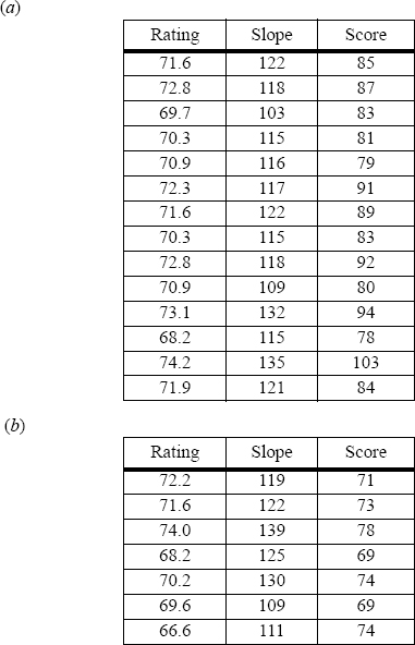
36. The handicap differential (HCD) for a round of golf is calculated from the formula:
![]()
The course rating and the slope are measures of how difficult a particular course is. A golfers handicap is calculated from a certain number N of their best (lowest) handicap scores according to the following table.

For example, if 13 rounds have been played, only the best five handicaps are used. A handicap cannot be computed for fewer than five rounds. If more than 20 rounds have been played, only the 20 most recent results are used.
Once the lowest N handicap differentials have been identified, they are averaged and then rounded down to the nearest tenth. The result is the player’s handicap. Write a program in a script file that calculates a person’s handicap. The program asks the user to enter the golfers record in a three columns matrix where the first column is the course rating, the second is the course slope, and the third is the player’s score. Each row corresponds to one round. The program displays the person’s handicap. Execute the program for players with the following records.