Chapter 3

Mathematical Operations with Arrays

Once variables are created in MATLAB they can be used in a wide variety of mathematical operations. In Chapter 1 the variables that were used in mathematical operations were all defined as scalars. This means that they were all 1 × 1 arrays (arrays with one row and one column that have only one element) and the mathematical operations were done with single numbers. Arrays, however, can be one-dimensional (arrays with one row, or with one column), two-dimensional (arrays with multiple rows and columns), and even of higher dimensions. In these cases the mathematical operations are more complex. MATLAB, as its name indicates, is designed to carry out advanced array operations that have many applications in science and engineering. This chapter presents the basic, most common mathematical operations that MATLAB performs using arrays.

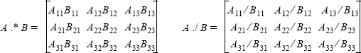
Addition and subtraction are relatively simple operations and are covered first, in Section 3.1. The other basic operations—multiplication, division, and exponentiation—can be done in MATLAB in two different ways. One way, which uses the standard symbols (*, /, and ^), follows the rules of linear algebra and is presented in Sections 3.2 and 3.3. The second way, which is called element-by-element operations, is covered in Section 3.4. These operations use the symbols .*, ./, and .^ (a period is typed in front of the standard operation symbol). In addition, in both types of calculations, MATLAB has left division operators ( . or ), which are also explained in Sections 3.3 and 3.4.

A Note to First-Time Users of MATLAB:

Although matrix operations are presented first and element-by-element operations next, the order can be reversed since the two are independent of each other. It is expected that almost every MATLAB user has some knowledge of matrix operations and linear algebra, and thus will be able to follow the material covered in Sections 3.2 and 3.3 without any difficulty. Some readers, however, might prefer to read Section 3.4 first. MATLAB can be used with element-by-element operations in numerous applications that do not require linear algebra multiplication (or division) operations.

3.1   ADDITION AND SUBTRACTION

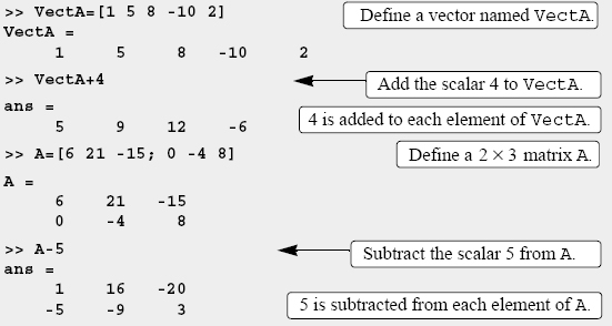
The operations + (addition) and − (subtraction) can be used to add (subtract) arrays of identical size (the same numbers of rows and columns) and to add (subtract) a scalar to an array. When two arrays are involved the sum, or the difference, of the arrays is obtained by adding, or subtracting, their corresponding elements.

In general, if A and B are two arrays (for example, 2 × 3 matrices),

then the matrix that is obtained by adding A and B is:

Examples are:

When a scalar (number) is added to (or subtracted from) an array, the scalar is added to (or subtracted from) all the elements of the array. Examples are:

3.2   ARRAY MULTIPLICATION

The multiplication operation * is executed by MATLAB according to the rules of linear algebra. This means that if A and B are two matrices, the operation A*B can be carried out only if the number of columns in matrix A is equal to the number of rows in matrix B. The result is a matrix that has the same number of rows as A and the same number of columns as B. For example, if A is a 4 × 3 matrix and B is a 3 × 2 matrix:

then the matrix that is obtained with the operation A*B has dimensions 4 × 2 with the elements:

A numerical example is:

The product of the multiplication of two square matrices (they must be of the same size) is a square matrix of the same size. However, the multiplication of matrices is not commutative. This means that if A and B are both n × n, then A*B ≠ B*A. Also, the power operation can be executed only with a square matrix (since A*A can be carried out only if the number of columns in the first matrix is equal to the number of rows in the second matrix).

Two vectors can be multiplied only if they have the same number of elements, and one is a row vector and the other is a column vector. The multiplication of a row vector by a column vector gives a 1 × 1 matrix, which is a scalar. This is the dot product of two vectors. (MATLAB also has a built-in function, dot(a,b), that computes the dot product of two vectors.) When using the dot function, the vectors a and b can each be a row vector or a column vector (see Table 3-1). The multiplication of a column vector by a row vector, each with n elements, gives an n × n matrix. Multiplication of array is demonstrated in Tutorial 3-1,

Tutorial 3-1: Multiplication of arrays.

When an array is multiplied by a number (actually a number is a 1 × 1 array), each element in the array is multiplied by the number. For example:

Linear algebra rules of array multiplication provide a convenient way for writing a system of linear equations. For example, the system of three equations with three unknowns

can be written in a matrix form as

and in matrix notation as

3.3   ARRAY DIVISION

The division operation is also associated with the rules of linear algebra. This operation is more complex, and only a brief explanation is given below. A full explanation can be found in books on linear algebra.

The division operation can be explained with the help of the identity matrix and the inverse operation.

Identity matrix:

The identity matrix is a square matrix in which the diagonal elements are 1s and the rest of the elements are 0s. As was shown in Section 2.2.1, an identity matrix can be created in MATLAB with the eye command. When the identity matrix multiplies another matrix (or vector), that matrix (or vector) is unchanged (the multiplication has to be done according to the rules of linear algebra). This is equivalent to multiplying a scalar by 1. For example:

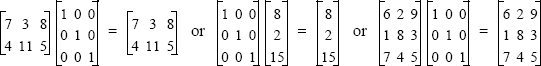
If a matrix A is square, it can be multiplied by the identity matrix, I, from the left or from the right:

AI = IA = A

Inverse of a matrix:

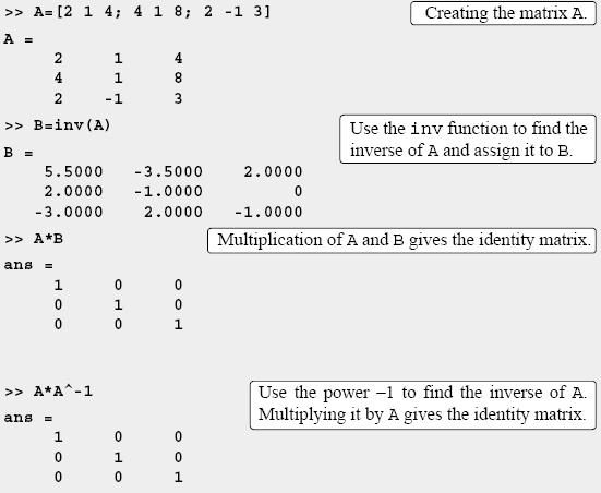
The matrix B is the inverse of the matrix A if, when the two matrices are multiplied, the product is the identity matrix. Both matrices must be square, and the multiplication order can be BA or AB.

BA = AB = I

Obviously B is the inverse of A, and A is the inverse of B. For example:

The inverse of a matrix A is typically written as A⁻¹. In MATLAB the inverse of a matrix can be obtained either by raising A to the power of −1, A⁻¹, or with the inv(A) function. Multiplying the matrices above with MATLAB is shown below.

Not every matrix has an inverse. A matrix has an inverse only if it is square and its determinant is not equal to zero.

Determinants:

A determinant is a function associated with square matrices. A short review on determinants is given below. For a more detailed coverage refer to books on linear algebra.

The determinant is a function that associates with each square matrix A a number, called the determinant of the matrix. The determinant is typically denoted by det(A) or |A|. The determinant is calculated according to specific rules. For a second-order 2 × 2 matrix, the rule is:

The determinant of a square matrix can be calculated with the det command (see Table 3-1).

Array division:

MATLAB has two types of array division, right division and left division.

Left division, :

Left division is used to solve the matrix equation AX = B. In this equation X and B are column vectors. This equation can be solved by multiplying, on the left, both sides by the inverse of A:

A⁻¹AX = A⁻¹B

The left-hand side of this equation is X, since

A⁻¹AX = IX = X

So the solution of AX = B is:

X = A⁻¹B

In MATLAB the last equation can be written by using the left division character:

X = AB

It should be pointed out here that although the last two operations appear to give the same result, the method by which MATLAB calculates X is different. In the first, MATLAB calculates A⁻¹ and then uses it to multiply B. In the second (left division), the solution X is obtained numerically using a method that is based on Gauss elimination. The left division method is recommended for solving a set of linear equations, because the calculation of the inverse may be less accurate than the Gauss elimination method when large matrices are involved.

Right division, / :

The right division is used to solve the matrix equation XC = D. In this equation X and D are row vectors. This equation can be solved by multiplying, on the right, both sides by the inverse of C:

X · CC⁻¹ = D · C⁻¹

which gives

X = D · C⁻¹

In MATLAB the last equation can be written using the right division character:

X = D/C

The following example demonstrates the use of the left and right division, and the inv function to solve a set of linear equations.

3.4   ELEMENT-BY-ELEMENT OPERATIONS

In Sections 3.2 and 3.3 it was shown that when the regular symbols for multiplication and division (* and /) are used with arrays, the mathematical operations follow the rules of linear algebra. There are, however, many situations that require element-by-element operations. These operations are carried out on each of the elements of the array (or arrays). Addition and subtraction are by definition already element-by-element operations, since when two arrays are added (or subtracted) the operation is executed with the elements that are in the same position in the arrays. Element-by-element operations can be done only with arrays of the same size.

Element-by-element multiplication, division, or exponentiation of two vectors or matrices is entered in MATLAB by typing a period in front of the arithmetic operator.

If two vectors a and b are a = [a₁ a₂ a₃ a₄] and b = [b₁ b₂ b₃ b₄], then element-by-element multiplication, division, and exponentiation of the two vectors gives:

If two matrices A and B are

then element-by-element multiplication and division of the two matrices give:

Element-by-element exponentiation of matrix A gives:

Element-by-element multiplication, division, and exponentiation are demonstrated in Tutorial 3-2.

Tutorial 3-2: Element-by-element operations.

Element-by-element calculations are very useful for calculating the value of a function at many values of its argument. This is done by first defining a vector that contains values of the independent variable, and then using this vector in element-by-element computations to create a vector in which each element is the corresponding value of the function. One example is:

In the example above y = x² − 4x. Element-by-element operation is needed when x is squared. Each element in the vector y is the value of y that is obtained when the value of the corresponding element of the vector x is substituted in the equation. Another example is:

In the last example . Element-by-element operations are used in this example three times: to calculate z³ and z², and to divide the numerator by the denominator.

3.5   USING ARRAYS IN MATLAB BUILT-IN MATH FUNCTIONS

The built-in functions in MATLAB are written such that when the argument (input) is an array, the operation that is defined by the function is executed on each element of the array. (One can think of the operation as element-by-element application of the function.) The result (output) from such an operation is an array in which each element is calculated by entering the corresponding element of the argument (input) array into the function. For example, if a vector with seven elements is substituted in the function cos(x), the result is a vector with seven elements in which each element is the cosine of the corresponding element in x. This is shown below.

An example in which the argument variable is a matrix is:

The feature of MATLAB in which arrays can be used as arguments in functions is called vectorization.

3.6   BUILT-IN FUNCTIONS FOR ANALYZING ARRAYS

MATLAB has many built-in functions for analyzing arrays. Table 3-1 lists some of these functions.

Table 3-1: Built-in array functions

3.7   GENERATION OF RANDOM NUMBERS

Simulations of many physical processes and engineering applications frequently require using a number (or a set of numbers) with a random value. MATLAB has three commands—rand, randn, and randi—that can be used to assign random numbers to variables.

The rand command:

The rand command generates uniformly distributed random numbers with values between 0 and 1. The command can be used to assign these numbers to a scalar, a vector, or a matrix, as shown in Table 3-2.

Table 3-2: The rand command

Sometimes there is a need for random numbers that are distributed in an interval other than (0,1), or for numbers that are integers only. This can be done using mathematical operations with the rand function. Random numbers that are distributed in a range (a,b) can be obtained by multiplying rand by (b – a) and adding the product to a:

(b – a)*rand + a

For example, a vector of 10 elements with random values between −5 and 10 can be created by (a = −5, b = 10):

The randi command:

The randi command generates uniformly distributed random integer. The command can be used to assign these numbers to a scalar, a vector, or a matrix, as shown in Table 3-3.

Table 3-3:  randi command

The range of the random integers can be set to be between any two integers by typing [imin imax] instead of imax. For example, a matrix with random integers between 50 and 90 is created by:

The randn command:

The randn command generates normally distributed numbers with mean 0 and standard deviation of 1. The command can be used to generate a single number, a vector, or a matrix in the same way as the rand command. For example, a 3 × 4 matrix is created by:

The mean and standard deviation of the numbers can be changed by mathematical operations to have any values. This is done by multiplying the number generated by the randn function by the desired standard deviation, and adding the desired mean. For example, a vector of six numbers with a mean of 50 and standard deviation of 6 is generated by:

Integers of normally distributed numbers can be obtained by using the round function.

3.8   EXAMPLE OF MATLAB APPLICATIONS

Sample Problem 3-2:   Equivalent force system (addition of vectors)

Three forces are applied to a bracket as shown. Determine the total (equivalent) force applied to the bracket.

Solution

A force is a vector (a physical quantity that has a magnitude and direction). In a Cartesian coordinate system a twodimensional vector F can be written as:

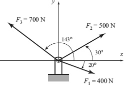
where F is the magnitude of the force and θ is its angle relative to the x axis, F_x and F_y are the components of F in the directions of the x and y axes, respectively, and i and j are unit vectors in these directions. If F_x and F_y are known, then F and θ can be determined by:

The total (equivalent) force applied on the bracket is obtained by adding the forces that are acting on the bracket. The MATLAB solution below follows three steps:

• Write each force as a vector with two elements, where the first element is the x component of the vector and the second element is the y component.
• Determine the vector form of the equivalent force by adding the vectors.
• Determine the magnitude and direction of the equivalent force.

The problem is solved in the following script file.

When the program is executed, the following is displayed in the Command Window:

The equivalent force has a magnitude of 589.98 N, and is directed 64.95° (ccw) relative to the x axis. In vector notation, the force is F = 249.84i + 534.46j N.

Sample Problem 3-3:   Friction experiment (element-by-element calculations)

The coefficient of friction, μ, can be determined in an experiment by measuring the force F required to move a mass m. When F is measured and m is known, the coefficient of friction can be calculated by:

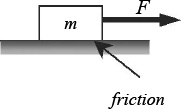
μ = F/(mg) (g = 9.81 m/s²).

Results from measuring F in six tests are given in the table below. Determine the coefficient of friction in each test, and the average from all tests.

Solution

A solution using MATLAB commands in the Command Window is shown below.

Sample Problem 3-4:   Electrical resistive network analysis (solving a system of linear equations)

The electrical circuit shown consists of resistors and voltage sources. Determine the current in each resistor using the mesh current method, which is based on Kirchhoff’s voltage law.

Solution

Kirchhoff’s voltage law states that the sum of the voltage around a closed circuit is zero. In the mesh current method a current is first assigned for each mesh (i₁, i₂, i₃, i₄ in the figure). Then Kirchhoff’s voltage law is applied for each mesh. This results in a system of linear equations for the currents (in this case four equations). The solution gives the values of the mesh currents. The current in a resistor that belongs to two meshes is the sum of the currents in the corresponding meshes. It is convenient to assume that all the currents are in the same direction (clockwise in this case). In the equation for each mesh, the voltage source is positive if the current flows to the – pole, and the voltage of a resistor is negative for current in the direction of the mesh current.

The equations for the four meshes in the current problem are:

The four equations can be rewritten in matrix form [A][x] = [B]:

The problem is solved in the following program, written in a script file:

When the script file is executed, the following is displayed in the Command Window:

The last column vector gives the current in each mesh. The currents in the resistors R₁, R₅, and R₈ are i₁ = 0.8411 A, i₂ = 0.7206 A, and i₄ = 1.5750 A, respectively. The other resistors belong to two meshes and their current is the sum of the currents in the meshes.

The current in resistor R₂ is i₁ − i₂ = 0.1205 A.

The current in resistor R₃ is i₁ − i₃ = 0.2284 A.

The current in resistor R₄ is i₂ − i₃ = 0.1079 A.

The current in resistor R₆ is i₄ − i₃ = 0.9623 A.

The current in resistor R₇ is i₄ − i₂ = 0.8544 A.

Sample Problem 3-5:   Motion of two particles

A train and a car are approaching a road crossing. At time t = 0 the train is 400 ft south of the crossing traveling north at a constant speed of 54 mi/h. At the same time the car is 200 ft west of the crossing traveling east at a speed of 28 mi/h and accelerating at 4 ft/s². Determine the positions of the train and the car, the distance between them, and the speed of the train relative to the car every second for the next 10 seconds.

To show the results, create an 11 × 6 matrix in which each row has the time in the first column and the train position, car position, distance between the train and the car, car speed, and the speed of the train relative to the car in the next five columns, respectively.

Solution

The position of an object that moves along a straight line at a constant acceleration is given by where s_o and v_o are the position and velocity at t = 0, and a is the acceleration. Applying this equation to the train and the car gives:

The distance between the car and the train is: . The velocity of the train is constant and in vector notation is given by v_train = v_otrainj. The car is accelerating and its velocity at time t is given by v_car = (v_ocar + a_cart)i. The velocity of the train relative to the car, v_t/c, is given by v_t/c = v_train − v_car = − (v_ocar + a_cart)i + v_otrainj. The magnitude (speed) of this velocity is the length of the vector.

The problem is solved in the following program, written in a script file. First a vector t with 11 elements for the time from 0 to 10 s is created, then the positions of the train and the car, the distance between them, and the speed of the train relative to the car at each time element are calculated.

Note: In the commands above, table is the name of the variable that is a matrix containing the data to be displayed.

When the script file is executed, the following is displayed in the Command Window:

In this problem the results (numbers) are displayed by MATLAB without any text. Instructions on how to add text to output generated by MATLAB are presented in Chapter 4.

3.9  PROBLEMS

Note:   Additional problems for practicing mathematical operations with arrays are provided at the end of Chapter 4.

1. For the function y = x² − e^0.5x + x, calculate the value of y for the following values of x using element-by-element operations: −3, −2, −1, 0, 1, 2, 3.

2. For the function , calculate the value of y for the following values of x using element-by-element operations: 1, 2, 3, 4, 5, 6.

3. For the function , calculate the value of y for the following values of x using element-by-element operations: 1.5, 2.5, 3.5, 4.5, 5.5, 6.6.

4. For the function , calculate the value of y for the following values of x using element-by-element operations: 20°, 30°, 40°, 50°, 60°, 70°.

5. The radius, r, of a sphere can be calculated from its surface area, s, by:

The volume, V, is given by:

Determine the volume of spheres with surface area of 50, 100, 150, 200, 250, and 300 ft². Display the results in a two-column table where the values of s and V are displayed in the first and second columns, respectively.

6. The electric field intensity, E(Z), due to a ring of radius R at any point z along the axis of the ring is given by:

where λ is the charge density, ε₀ = 8085 × 10⁻¹² is the electric constant, and R is the radius of the ring. Consider the case where λ = 1.7 × 10⁻⁷ C/m and R = 6cm.

(a) Determine at E(z) at z = 0, 2, 4, 6, 8, and 10 cm.

(b) Determine the distance z where E is maximum. Do it by creating a vector z with elements ranging from 2 cm to 6 cm and spacing of 0.01 cm. Calculate E for each value of z and then find the maximum E and associated z with MATLAB’s built-in function max.

7. The voltage V_c(t) (in V) and the current i(t) (in Amp) t seconds after closing the switch in the circuit shown are given by:

where τ₀ = RC is the time constant. Consider the case where V₀ = 24V, R = 3800 Ω and C = 4000 × 10⁻⁶ F. Determine the voltage and the current during the first 20 s after the switch is closed. Create a vector with values of times from 0 to 20 s with spacing of 2 s, and use it for calculating V_c(t) and i(t). Display the results in a three-column table where the values of time, voltage and current are displayed in the first, second, and third columns, respectively.

8. The length |u| (magnitude) of a vector u = xi + yj + zk is given by . Given the vector u = 23.5i − 17j + 6k, determine its length in the following two ways:

(a) Define the vector in MATLAB, and then write a mathematical expression that uses the components of the vector.

(b) Define the vector in MATLAB, then determine the length by writing one command that uses element-by-element operation and MATLAB built-in functions sum and sqrt.

9. A vector w_L of length L in the direction of a vector u = xi + yj + zk can determined by w_L = Lu_n (multiplying a unit vector in the direction of u by L). The unit vector u_n in the direction of the vector u is given by . By writing one MATLAB command, determine a vector of length 18 in the direction of the vector u = 7i − 4j − 11k.

10. The following two vectors are defined in MATLAB:

v = [15, 8, −6]       u = [3, −2, 6]

By hand (pencil and paper) write what will be displayed if the following commands are executed by MATLAB. Check your answers by executing the commands with MATLAB.

(a) v./u

(b) u′*v

(c) u*v′

11. Two vectors are given:

u = 5i − 6j + 9k     and     v = 11i + 7j − 4k

Use MATLAB to calculate the dot product u · v of the vectors in three ways:

(a) Write an expression using element-by-element calculation and the MATLAB built-in function sum.

(b) Define u as a row vector and v as a column vector, and then use matrix multiplication.

(c) Use the MATLAB built-in function dot.

12. Define the vector v = [2  3 4  5  6]. Then use the vector in a mathematical expression to create the following vectors:

(a)  a = [4 6 8 10 12]

(b)  b = [8 27 64 125 216]

(c)  c = [2² 3³ 4⁴ 5⁵ 6⁶]

(d)  d = [1 1.5 2 2.5 3]

13. Define the vector v = [8 6 4 2]. Then use the vector in a mathematical expression to create the following vectors:

14. Define x and y as the vectors and x = [1, 2, 3, 4, 5] and y = [2, 4, 6, 8, 10]. Then use them in the following expressions to calculate z using element-by-element calculations.

15. Define r and s as scalars and r = 1.6 × 10³ and s = 14.2, and, t, x, and y as vectors t = [1, 2, 3, 4, 5], x = [0, 2, 4, 6, 8], and y = [3, 6, 9, 12, 15]. Then use these variables to calculate the following expressions using element-by-element calculations for the vectors.

16. The area of a triangle ABC can be calculated by |r_AB × r_AC|/2, where r_AB and r_AC are vectors connecting the vertices A and B and C, respectively. Determine the area of the triangle shown in the figure. Use the following steps in a script file to calculate the area. First, define the vectors r_OA, r_OB and r_OC from knowing the coordinates of points A, B, and C. Then determine the vectors r_AB and r_AC from r_OA, and r_OB and r_OC. Finally, determine the area by using MATLAB’s built-in functions cross, sum. and sqrt.

17. The volume of the parallelepiped shown can be calculated by r_OB · (r_OA × r_AC). Use the following steps in a script file to calculate the area. Define the vectors r_OA, r_AC, and r_OB from knowing position of points A, B, and C. Determine the volume by using MATLAB’s built-in functions dot and cross.

18. Define the vectors:

u = 5i − 2j + 4k,   v = −2i + 7j + 3k, and w = 8i + 1j − 3k

Use the vectors to verify the identity:

(u + v) · [(v + w) × (w + u)] = 2u · (v × w)

Use MATLAB’s built-in functions cross and dot, calculate the value of the left and right sides of the identity.

19. The dot product can be used for determining the angle between two vectors:

Use MATLAB’s built-in functions acosd, sqrt, and dot to find the angle (in degrees) between r₁ = 6i − 3j + 2k and r₂ = 2i + 9j + 10k. Recall that .

20 Use MATLAB to show that the angle inscribed in a semi-circle is a right angle. Use the following steps in a script file to calculate the angle. Define a variable with the value of the x coordinate of point A. Determine the y coordinate of point A using the equation x² + y² = R². Define vectors that correspond to the position of points A, B, and C and use them for determining position vectors r_AB and r_AC. Calculate the angle α in two ways.

First by using the equation , and then by using the equation . Both should give 90°.

21. The position as a function of time (x(t), y(t))of a projectile fired with a speed of v₀ at an angle α is given by

where g = 9.81 m/s². The polar coordinates of the projectile at time t are (r(t), θ(t)), where and . Consider the case where v₀ = 162m/s and α = 70°. Determine r(t) and θ(t) for t = 1, 6, 11, …, 31s.

22. Use MATLAB to show that the sum of the infinite series converges to e². Do this by computing the sum for:

(a) n = 5,

(b) n = 10,

(c) n = 50

For each part create a vector n in which the first element is 0, the increment is 1 and the last term is 5, 10, or 50. Then use element-by-element calculations to create a vector in which the elements are . Finally, use MATLAB’s built-in function sum to sum the series. Compare the values to e² (use format long to display the numbers).

23. Use MATLAB to show that the sum of the infinite series converges to 10. Do this by computing the sum for

(a) n = 10,

(b) n = 50,

(c) n = 100

For each part, create a vector n in which the first element is 1, the increment is 1 and the last term is 10, 50 or 100. Then use element-by-element calculations to create a vector in which the elements are . Finally, use MATLAB’s built-in function sum to sum the series. Compare the values to (use format long to display the numbers).

24. According to Zeno’s paradox any object in motion must arrive at the halfway point before it can arrive at its destination. Once arriving at the halfway point, the remaining distance is once again divided in half and so on to infinity. Since it is impossible to complete this process, Zeno concluded all motion must be an illusion. Letting the length be unity, Zeno’s paradox can be written in terms of the infinite sum . To see how quickly this series converges to 1, compute the sum for:

(a) n = 5,

(b) n = 10,

(c) n = 40

For each part create a vector n in which the first element is 1, the increment is 1, and the last term is 5, 10, or 40. Then use element-by-element calculations to create a vector in which the elements are . Finally, use the MATLAB built in function sum to add the terms of the series. Compare the values obtained in parts (a), (b), and (c) with the value of 1.

25. Show that .

Do this by first creating a vector x that has the elements 1.0, 0.5, 0.1, 0.01, 0.001, and 0.0001. Then, create a new vector y in which each element is determined from the elements of x by . Compare the elements of y with the value 4 (use format long to display the numbers).

26. Show that .

Do this by first creating a vector x that has the elements 2.0, 1.5, 1.1, 1.01, 1.001, 1.00001, and 1.0000001. Then, create a new vector y in which each element is determined from the elements of x by . Compare the elements of y with the value 4/3 (use format long to display the numbers).

27. The demand for water during a fire is often the most important factor in the design of distribution storage tanks and pumps. For communities with populations less than 200,000, the demand Q (in gallons/min) can be calculated by:

where P is the population in thousands. Set up a vector for P that starts at 10 and increments by 10 up to 200. Use element-by-element computations to determine the demand Q for each population in P.

28. The ideal gas equation states that , where P is the pressure, V is the volume, T is the temperature, R = 0.08206(L atm)/(mol K) is the gas constant, and n is the number of moles. Real gases, especially at high pressure, deviate from this behavior. Their response can be modeled with the van der Waals equation

where a and b are material constants. Consider 1 mole (n = 1) of nitrogen gas at T = 300K. (For nitrogen gas (L² atm)/mol², and b = 0.0391 L/mol.) Create a vector with values of Vs for 0.1 ≤ V ≤ 1 L, using increments of 0.02 L. Using this vector calculate P twice for each value of V, once using the ideal gas equation and once with the van der Waals equation. Using the two sets of values for P, calculate the percent of error for each value of V. Finally, by using MATLAB’s built-in function max, determine the maximum error and the corresponding volume.

29. Create the following three matrices:

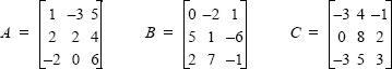
(a) Calculate A + B and B + A to show that addition of matrices is commutative.

(b) Calculate A + (B + C) and (A + B) + C to show that addition of matrices is associative.

(c) Calculate 3(A + C) and 3A + 5C to show that, when matrices are multiplied by a scalar, the multiplication is distributive.

(d) Calculate A*(B + C) and A*B + A*C to show that matrix multiplication is distributive.

30. Use the matrices A, B, and C from the previous problem to answer the following:

(a) Does A*B = B*A?

(b) Does A*(B*C = (A*B)*C?

(c) Does (A*B)^t = A^t*B^t? (^t means transpose)

(d) Does (A + B)^t = A^t + B^t?

31. Create a 4 × 4 matrix A having random integer values between 1 and 10. Call the matrix A and, using MATLAB, perform the following operations. For each part explain the operation.

(a) A * A

(b) A. *A

(c) A A

(d) A. / A

(e) det (A)

(e) inv (A)

32. The magic square is an arrangement of numbers in a square grid in such a way that the sum of the numbers in each row, and in each column, and in each diagonal is the same. MATLAB has a built-in function magic(n) that returns an n × n magic square. In a script file create a (6 × 6) magic square, and then test the properties of the resulting matrix by finding the sum of the elements in each row, in each column and in both diagonals. In each case, use MATLAB’s built-in function sum. (Other functions that can be useful are diag and fliplr.)

33. Solve the following system of three linear equations:

34. Solve the following system of five linear equations:

35. A food company manufactures five types of 8 oz Trail mix packages using different mixtures of peanuts, almonds, walnuts, raisins, and M&Ms. The mixtures have the following compositions:

How many packages of each mix can be manufactured if 128 lb of peanuts, 118 lb of almonds, 112 lb of walnuts, 112 lb of raisins, and 104 lb of M&Ms are available? Write a system of linear equations and solve.

36. The electrical circuit shown consists of resistors and voltage sources. Determine i₁, i₂, i₃, and i₄, using the mesh current method based on Kirchhoff’s voltage law (see Sample Problem 3-4).

37. The electrical circuit shown consists of resistors and voltage sources. Determine i₁, i₂, i₃, i₄ and i₅, using the mesh current method based on Kirchhoff’s voltage law (see Sample Problem 3-4).