Chapter 5
Modern Data Warehouses in Azure
Chapter 1, “Core Data Concepts,” and Chapter 2, “Relational Databases in Azure,” examine the fundamental concepts of analytical workloads, including common definitions and design patterns. This chapter expands on these concepts by exploring the various components that can be involved in Azure-based analytical workloads. These components include services that are involved in ingesting and processing data and storage options for a modern data warehouse.
Analytical Workload Features
Throughout this book we have covered the features and design considerations used by different workload types. For this reason, the following sections will only provide a summary of the different workload types. The important takeaway for this chapter is how analytical workloads differentiate from transactional ones and how batch and stream processing are used in a modern data warehouse solution. Understanding these features will set the stage for the rest of the chapter when we examine how to build modern data warehouses in Azure.
Transactional vs. Analytical Workloads
Analytical workloads can be built using many of the same technologies and components as transactional workloads. However, there are several design practices and features that are more optimal for one over the other. When designing a modern data warehouse, it is important to consider what sets analytical and transactional workloads apart.
Transactional Workload Features
As discussed in Chapter 1, “Core Data Concepts,” online transaction processing (OLTP) systems capture the business transactions that support the data-to-day operations of a business. Data stores that are used for OLTP systems must be able to handle millions of transactions a day while ensuring that none of the data is corrupted. Traditionally, OLTP systems have always been hosted on relational databases as these platforms implement ACID properties to ensure data integrity.
Relational databases supporting OLTP systems are highly normalized, typically following third normal form (3NF), separating related data into multiple tables to eliminate data redundancy. This design standard ensures that database tables are optimized for write operations. While this level of normalization is ideal for write operations, it is less efficient for analytical workloads that perform read-heavy operations. Analysts who have built reports from databases that are designed for OLTP workloads will inevitably be forced to write complicated queries that use several join operations to create the desired result set. This can lead to bad performance and concurrency issues with write operations.
Before examining features and best practices for analytical workloads, it is important to note that not all OLTP workloads are suitable for highly normalized, relational databases. Transactional data that is produced in large volumes and at high speeds can take a performance hit when being conformed to a fixed, normalized schema. In these cases, organizations can choose to host their transactional workloads on NoSQL document databases such as the Azure Cosmos DB Core (SQL) API. These databases store data in its original state as semi-structured documents, enabling transactions to be written to them very quickly.
While document databases are extremely efficient data stores for large volume and high velocity write operations, the lack of a consistent structure makes them difficult to use with analytical applications like reporting tools. Useful data fields are typically extrapolated from semi-structured NoSQL documents and stored in a format that is optimized for read-heavy operations. Several modern analytical services can also leverage data virtualization techniques to structure data for reporting applications while leaving the data in its source data store.
Analytical Workload Features
Analytical workloads are designed to help business users make data-driven decisions. These systems are used to answer several questions about the business: What has happened over the previous period? Why did particular events happen? What will happen if all things stay the same? What will happen if we make specific changes in different areas? As discussed in Chapter 1, these questions are answered by the different types of analytics that make up the analytics maturity model.
Data-driven business decisions come from extracting useful information from several source data stores, including OLTP databases. Once extracted, source data will typically undergo several transformation steps to remove extraneous features and remediate data quality issues. Cleansed data is then conformed to an easy-to-use data model for analytics. Data that is ready to be analyzed is stored in a relational data warehouse, an OLAP model, or as files in an enterprise data lake.
Reporting applications and analytical applications used to analyze historical data typically retrieve data from read optimized data stores such as a data warehouse or an OLAP model. Many of these systems offer in-memory and column-based storage capabilities that are optimal for analytical queries that aggregate large amounts of data. Data warehouses and department-specific data marts are built with relational databases like Azure Synapse Analytics dedicated SQL pools or Azure SQL Database. Unlike OLTP data stores that are built with relational databases, data warehouses use a denormalized data model. The section “Data Modeling Best Practices for Data Warehouses” later in this chapter covers this approach in further detail.
While most analytical workloads store processed data used by reporting applications in a relational data warehouse such as Azure Synapse Analytics dedicated SQL pools or an OLAP tool such as Azure Analysis Services, many organizations choose to store data used by data scientists as files in an enterprise data lake. Cloud-based data lakes such as Azure Data Lake Store Gen2 (ADLS) can store massive amounts of data much cheaper than a relational data warehouse. Data lakes can also store large amounts of unstructured data such as images, video, and audio that data scientists can leverage with deep learning techniques. Data architects can take advantage of these capabilities by providing data scientists with large volumes and several types of data that they can use to build insightful machine learning models.
Modern cloud-based analytical workloads typically use a combination of an enterprise data lake and a data warehouse. Relational database engines used to host data warehouses offer faster query performance, higher user concurrency, and more granular security than data lake technologies. On the other hand, data lake services can host unlimited amounts data at a much cheaper cost, allowing users to store multiple copies of data to leverage for several different use cases. Data lakes can also store a wide variety of data, allowing users to interact with semi-structured and unstructured data with relative ease. This is why most organizations store all of their data in an enterprise data lake and only load data that is necessary for reporting from the data lake into a data warehouse.
In recent years, several technologies have been introduced that are optimized for ad hoc analysis with data stored in a data lake. By storing data using a columnar format such as Parquet, analysts can leverage data virtualization technologies such as Azure Synapse Analytics serverless SQL pools to query their data with T-SQL without having to create a separate copy of the data in a relational database. Data engineers can also store data in ADLS with Delta Lake. Delta Lake is an open-source storage layer that enables ACID properties on Parquet files in ADLS. This ensures data integrity for data stored in ADLS, perfect for ad hoc analysis and data science initiatives. More information about Delta Lake and the “Lakehouse” concept can be found at https://delta.io.
While using a data lake like a data warehouse can serve as a relational database replacement with smaller workloads, large reporting workloads that analyze data from several sources can benefit from the performance of a relational database. You can find more information about the benefits of using a relational data warehouse and a data lake together in the following blog post from James Serra: www.jamesserra.com/archive/2020/09/data-lakehouse-synapse.
Data used by analytical workloads have to go through a data processing workflow before it eventually lands in a data lake and/or a data warehouse. Even if the data does not undergo any transformations, it still needs to be extracted and loaded into a destination data store. Data engineers can use one or a combination of the following data processing techniques to create an end-to-end data pipeline: batch processing and stream processing.
Data Processing Techniques
Batch and stream processing are two data processing techniques that are used to manipulate data at rest and in real time. As discussed in Chapter 1, these techniques can be leveraged together in modern data processing architectures such as the Lambda architecture. This empowers organizations to make decisions with a wide variety of data that is generated at different speeds. Let's examine each of these techniques further in the following sections before exploring how they can be used in the same solution.
Batch Processing
Batch processing activities act on groups, or batches, of data at predetermined periods of time or after a specified event. One example of batch processing is a retail company processing daily sales every night and loading the transformed data into a data warehouse. The following list included reasons for why you would want to use batch processing:
- Working with large volumes of data that require a significant amount of compute power and time to process
- Running data processing activities during off-hours to avoid inaccurate reporting
- Processing data every time a specific event occurs, such as a blob being uploaded to Azure Blob storage
- Transforming batches of semi-structured data, such as JSON or XML, into a structured format that can be loaded into a data warehouse
- Processing data that is related to business intervals, such as yearly/quarterly/monthly/weekly aggregations
Data architects can implement batch processing activities using one of two techniques: extract, transform, and load (ETL) or extract, load, and transform (ELT). ETL pipelines extract data from one or more source systems, transform the data to meet user specifications, and then load the data in an analytical data store. ELT processes flip the transform and load stages and allow data engineers to transform data in the analytical data store. Because the ELT pattern is optimized for big data workloads, the analytical data store must be capable of working on data at scale. For this reason, ELT pipelines commonly use MPP technologies like Azure Synapse Analytics as the analytical data store.
Batch processing workflows in the cloud generally use the following components:
- Orchestration engine—This component manages the flow of a data pipeline. It handles when and how a pipeline starts, extracting data from source systems and landing it in data lake storage, and executing transformation activities. Developers can also leverage error handling logic in the orchestration engine to control how pipeline activity errors are managed. Depending on the design, orchestration engines can also be used to move transformed data into an analytical data store. Azure Data Factory (ADF) is a common service used for this workflow component.
- Object storage—This is a distributed data store, or data lake, that hosts large amounts of files in various formats. Developers can use data lakes to manage their data in multiple stages. This can include a bronze layer for raw data extracted directly from the source, a silver layer that represents the data after being scrubbed of any data quality issues, and a gold layer that stores an aggregated version of the data that has been enriched with domain-specific business rules. ADLS or Azure Blob Storage can be used for this workflow component.
- Transformation activities—This is a computational service that is able to process long-running batch jobs to filter, aggregate, normalize, and prepare data for analysis. These activities read source data from data lake storage, process it, and write the output back to data lake storage or an analytical data store. Azure Databricks, Azure HDInsight, Azure Synapse Analytics, and ADF mapping data flows are just a few examples of compute services that can transform data.
- Analytical data store—This is a storage service that is optimized to serve data to analytical tools such as Power BI. Azure services that can be used as an analytical data store include Azure Synapse Analytics and Azure SQL Database.
- Analysis and reporting—Reporting tools and analytical applications are used to create infographics with the processed data. Power BI is one example of a reporting tool used in a batch processing workflow.
Figure 5.1 illustrates an example of a batch processing workflow that uses ADF to extract data from a few source systems, lands the raw data in ADLS, processes the data with a combination of Azure Databricks and ADF mapping data flows, and finally loads the processed data into an Azure Synapse Analytics dedicated SQL pool.

FIGURE 5.1 Batch processing example
Stream Processing
Stream processing is a data processing technique that involves ingesting a continuous stream of data and performing computations on the data in real time. It is used for processing scenarios that have very short latency requirements, typically measured in seconds or milliseconds. Data that is ready for analysis is either sent directly to a dashboard or loaded into a persistent data store such as ADLS or Azure Synapse Analytics dedicated SQL pool for long-term analysis. Some examples of stream processing are listed here:
- Analyzing click-stream data to make recommendations in real-time
- Observing biometric data with fitness trackers and other IoT devices
- Monitoring offshore drilling equipment to detect any anomalies that indicate it needs to be repaired or replaced
Cloud-based stream processing workflows generally use the following components:
- Real-time message ingestion—This component captures data as messages in real time from different technologies that generate data streams. Azure Event Hubs and Azure IoT Hub are two PaaS offerings that data architects can use for real-time message ingestion. Several organizations leverage Apache Kafka, a popular open-source message ingestion platform, to process data streams. Organizations can move their existing Kafka workloads to Azure with the Azure HDInsight Kafka cluster type or the Azure Events for Kafka protocol.
- Stream processing—This component transforms, aggregates, and prepares data streams for analysis. These technologies can also load data in persistent data stores for long-term analysis. Azure Stream Analytics and Azure Functions are two PaaS offerings that data engineers can use to receive data from a real-time ingestion services and apply computations on the data.
- Apache Spark—This is a popular open-source data engineering platform that supports batch and stream processing. Stream processing is performed with the Spark structured streaming service, a processing service that transforms data streams as micro-batches in real time. Spark structured streaming jobs can be developed with Azure Databricks, the Azure HDInsight Spark cluster type, or an Azure Synapse Analytics Apache Spark pool. The collaborative nature and ease of use with Azure Databricks makes it the preferred service for Spark structured streaming jobs.
- Object storage—Data streams can be loaded into object storage to be archived or combined with other datasets for batch processing. Stream processing services can use an object store such as ADLS or Azure Blob Storage as a destination, or sink, data store for processed data. Some real-time ingestion services such as Azure Event Hubs can load data directly into object storage without the help of a stream processing service. This is useful for organizations that need to store the raw data streams for long-term analysis.
- Analytical data store—This is a storage service that serves processed data streams to analytical applications. Azure Synapse Analytics, Azure Cosmos DB, and Azure Data Explorer are services in Azure that can be used as an analytical data store for data streams.
- Analysis and reporting tools—Processed data can be written directly to a reporting tool such as a Power BI dashboard for instant analysis.
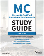
As discussed in Chapter 1, stream processing workflows can use one of two approaches: live or on demand. The “live” approach is the most commonly used pattern, processing data continuously as it is generated. The “on-demand” approach persists incoming data in object storage and processes it in micro-batches. An example of this approach is illustrated in Figure 5.2.
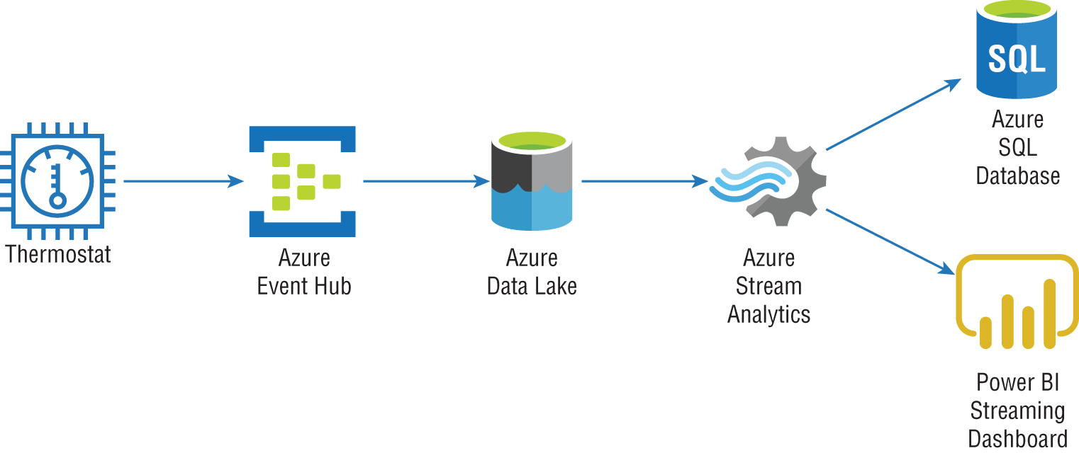
FIGURE 5.2 On-demand stream processing example
Modern Data Solutions with Batch and Stream Processing
Azure data services make it easy for data architects to use batch and stream processing workflows in the same solution. This flexibility gives business units the ability to quickly make well informed decisions from their data. These cloud-native solutions are designed with modern data processing patterns like the Lambda architecture.
The Lambda architecture is a data processing pattern that provides a framework for how users can use a combination of batch and stream processing for data analysis. Solutions that use the Lambda architecture separate batch and stream processing operations into a cold and hot path. Figure 5.3 illustrates the components and process flow used by the Lambda architecture.
The cold path, also known as the batch layer, manages all operations that are not constrained by low latency requirements. Batch layer operations typically process large datasets at predetermined periods of time. Once processed, data is loaded into the serving layer (e.g., an analytical data store like Azure Synapse Analytics) to be analyzed by reporting and analytical applications.
The hot path, also known as the speed layer, manages stream processing operations. Data is immediately processed and is either directly sent to a reporting application for instant analysis or loaded into the serving layer and combined with data processed in the batch layer.

FIGURE 5.3 Lambda architecture workflow
Modern Data Warehouse Components
Modern data warehouse solutions are more than just a simple analytical data store. They are made up of several components that give users flexible options for how they can analyze their data. Technologies used by modern data warehouse solutions are designed to scale horizontally as well as vertically, meaning that they can process and store very large datasets. Modern computing paradigms that enable these technologies to manage large and diverse datasets have also led to more dynamic design patterns. As discussed previously in this chapter, modern data warehouse solutions can combine batch and stream processing workflows with the Lambda architecture.
Cloud platforms such as Azure make building these solutions more accessible than ever before. Instead of having to procure hardware and spend the time configuring distributed services such as Hadoop or Spark to work in an on-premises environment, users can quickly deploy services that are designed to be core components of a modern data warehouse solution. Azure's pay-per-use cost model and the ability to quickly scale or delete services allow organizations to test different modern data warehouse components by completing short projects known as proofs of concept (POCs). POCs enable users to evaluate critical design decisions without having to make any large upfront hardware commitments.
The following sections explore data modeling best practices for the most commonly used Azure services for modern data warehouse solutions.
Data Modeling Best Practices for Data Warehouses
Data warehouses are data management systems that support analytical workloads and business intelligence (BI) activities. Data managed by a data warehouse is derived from several sources, such as OLTP systems, web APIs, IoT devices, and social media networks. Unlike OLTP systems, data warehouses use data models that are read-optimized so analytical queries issued against them can efficiently return aggregated calculations to support business decisions.
As discussed in Chapter 2, data warehouses use denormalized data models that are optimized for analytical queries and read-heavy workloads. The most common design practice for this approach is the star schema. Star schemas denormalize business data to minimize the number of tables in the data model. Tables consist of business entities and measurable events that are related to those entities. This division of data categories is represented by the two types of tables defined in the star schema: dimension tables and fact tables.
Dimension tables contain information that describes a particular business entity. These tables are typically very wide, containing several descriptor columns and a key column that serves as a unique identifier. Some common entities that are stored as dimension tables include date, customer, product category, and product subcategory information. In all of these cases, there could be a relatively small number of rows but a large number of columns to provide as much descriptive information as possible.
Fact tables store quantifiable observations that are related to the dimension tables. These tables can grow to be very large, comprising several millions of rows related to specific measurable events. Some fact table examples include Internet sales, product inventory, and weather metrics. Fact tables also include foreign key columns that are used to establish relationships with dimension tables. These relationships determine the level of granularity that analytical queries can use when filtering fact table data. For example, a query that is filtering an Internet sales fact table by a date dimension can only return time slices for the level of detail contained in the date dimension.
Azure Services for Modern Data Warehouses
In the Azure ecosystem there are several services that can be used to build a modern data warehouse solution. Depending on the scenario and the skillset of the engineers building the solution, most Azure services can be used to build different components of a data processing pipeline. However, there is a set of core Azure data services that are specifically designed to process big data workloads:
- Azure Data Factory
- Azure HDInsight
- Azure Databricks
- Azure Synapse Analytics
Each of these services can perform a variety of different functions in a data processing pipeline. This versatility allows them to be used in various stages of ETL or ELT pipelines. They have the flexibility to manage data in a variety of different formats and can scale horizontally as well as vertically to process very large volumes of data.
First, let's examine how Azure HDInsight, Azure Databricks, and ADF are used in modern data warehouse solutions. End-to-end data processing solutions with Azure Synapse Analytics will be described in the section “End-to-End Analytics with Azure Synapse Analytics” later in this chapter.
Azure HDInsight
Azure HDInsight is a managed, open-source analytics service in Azure. With Azure HDInsight, you can deploy distributed clusters for Apache Hadoop, Apache Spark, Apache Interactive Query/LLAP (Live Long and Process), Apache Kafka, Apache Storm, and Apache HBase in Azure. Being able to quickly stand up these environments without having to procure and manage hardware reduces the barriers to entry for organizations who are beginning to build a modern data warehouse.
Open-source frameworks like Hadoop and Spark are designed to handle large-scale data processing activities by using a scale-out architecture. While they can be installed on a single server node for test purposes, most use cases leverage multiple server nodes that are clustered together to perform processing activities at scale. Clusters consist of a head/driver node that divides jobs into smaller tasks and one or more worker nodes that execute each task.
Distributed frameworks also rely on resource managers like Apache Hadoop YARN (Yet Another Resource Negotiator) to manage cluster resources and job scheduling. Resource managers designate compute resources (such as CPU, memory, IO) to cluster nodes and monitor the resource usage. Knowing details of how YARN and other resource managers are designed is beyond the scope of the DP-900 exam and this book, but you can find more information at the following link if you would like to learn more: https://hadoop.apache.org/docs/current/hadoop-yarn/hadoop-yarn-site/YARN.html.
Azure HDInsight makes it easy to manage distributed frameworks like Hadoop and Spark and offers the capability to customize a cluster deployment, such as adding new components and languages. Also, since Azure HDInsight is a PaaS service, you can easily scale the number of worker nodes allocated to cluster up or down to increase compute power or cut back on cost.
It is important to understand the different Azure HDInsight cluster types and when you should use them. Also, keep in mind that after you have deployed an Azure HDInsight cluster, you will not be able to change the cluster type. For this reason, it is critical that you understand the scenarios the cluster will be supporting. The following list describes each of the cluster types supported by Azure HDInsight:
- Apache Hadoop is an open-source technology for distributed data processing. It uses the MapReduce parallel processing framework to process data at scale and the Hadoop Distributed File System (HDFS) as a distributed storage system. MapReduce jobs divide compute jobs into smaller units of work to be run in parallel across the various nodes in a cluster. Users can also leverage Apache Hive with Hadoop to project a schema on data and query data using HiveQL. More information about Apache Hive can be found at
https://docs.microsoft.com/en-us/azure/hdinsight/hadoop/hdinsight-use-hive.One drawback to Hadoop is that it only supports batch processing, forcing users to leverage another service like Apache Storm or Apache Spark for distributed stream processing. Hadoop also reads and writes data from and to disk, potentially leading to poorer processing performance than Apache Spark, which supports in-memory processing.
- Apache Spark is an open-source, distributed processing framework that supports in-memory processing. Because of its speed, Spark has become the standard framework for batch and stream distributed processing activities over Hadoop. Apache Spark also supports interactive querying capabilities, allowing users to easily query data from distributed data stores like ADLS with popular development languages like Spark SQL. More Spark-specific features such as development languages, workflows, and best practices will be described in the section “Azure Databricks.”
- Apache Kafka is an open-source, distributed real-time data ingestion platform that is used to build stream processing data pipelines. It offers message broker functionality that allows users to publish and subscribe to data streams.
- Apache HBase is an open-source NoSQL database that is built on top of Apache Hadoop. It uses a columnar format to store rows of data as column families, similar to the Azure Cosmos DB Cassandra API. Developers can interact with HBase data using Hive queries.
- Apache Storm is an open-source, real-time processing system for processing large data streams very quickly. Similar to Hadoop and Spark, it uses a distributed framework to parallelize stream processing jobs.
- Apache Interactive Query is an open-source, in-memory caching service for interactive and faster Hive queries. This cluster type can be used by developers or data scientists to easily run Hive queries against large datasets stored in Azure Blob Storage or ADLS.
As with any service in Azure, you can configure and deploy an Azure HDInsight cluster through the Azure Portal, through an Azure PowerShell or Azure CLI script, or via an Infrastructure as Code template like ARM or Bicep. Creating an Azure HDInsight cluster in Azure deploys the service chosen as the cluster type, the Apache Hadoop YARN resource manager to manage cluster resources, and several popular open-source tools such as Ambari, Avro, Hive, Sqoop, Tez, Pig, and Zookeeper. This greatly reduces the time it takes to get started building distributed solutions.
Most modern data warehouse scenarios leverage Apache Spark over Apache Hadoop, Apache Storm, and Apache Interactive Query to process large datasets due to its speed, ability to perform batch and stream processing activities, number of data source connectors, and overall ease of use. As a matter of fact, ADF mapping data flows use Apache Spark clusters to perform ETL activities. Apache Spark also enables data scientists and data analysts to interactively manipulate data concurrently.
There are a few management aspects that must be considered when deploying an Azure HDInsight cluster:
- Once provisioned, Azure HDInsight clusters cannot be paused. This means that you will need to delete the cluster if you want to save on costs when clusters are not being used. Organizations typically use an automation framework like Azure Automation to delete their clusters with Azure PowerShell or Azure CLI once they have finished running. They can then redeploy the cluster using an automation script or an Infrastructure as Code template.
- The lack of a pause feature for clusters creates a dilemma for metadata management. Azure HDInsight clusters use an Azure SQL Database as a central schema repository, also known as a metastore. The default metastore is tied to the life cycle of a cluster, meaning that when the cluster is deleted, the metastore and all information pertaining to Hive table schemas are deleted too. This can be avoided by using your own Azure SQL Database as a custom metastore. Custom metastores are not tied to the life cycle of a cluster, allowing you to create and delete clusters without losing any metadata. They can also be used to manage the Hive table schemas for multiple clusters. More information about custom metastores can be found at
https://docs.microsoft.com/en-us/azure/hdinsight/hdinsight-use-external-metadata-stores#custom-metastore. - Clusters do not support Azure AD authentication, RBAC, and multi-user capabilities by default. These services can be integrated by adding the Enterprise Security Package (ESP) to your cluster as part of the deployment workflow. More information about the ESP can be found at
https://docs.microsoft.com/en-us/azure/hdinsight/enterprise-security-package.
Later in this chapter we will discuss two other Azure services that can be used to build Apache Spark clusters. Azure Databricks and Azure Synapse Apache Spark pools are two Apache Spark–based analytics platforms that overcome the management overhead presented by Azure HDInsight. Both services allow you to easily pause (referred to as “terminate” in Azure Databricks) Spark clusters and maintain schema metadata without needing a custom external metastore. They are also natively integrated with Azure AD, enabling users to leverage their existing authentication/authorization mechanisms. Because of the ease of use and the additional components that provide a unified development experience for data engineers, Azure Databricks and Azure Synapse Analytics are the preferred choices for Apache Spark workloads. Reasons to use Azure Databricks instead of Azure Synapse Analytics Apache Spark pools and vice versa will be described in the following sections.
Azure HDInsight clusters are typically used in scenarios where Azure Databricks and Azure Synapse Analytics cannot be used or if Apache Kafka is required. The most common example of a scenario where Azure Databricks and Azure Synapse Analytics cannot be used is a solution that requires its Azure resources to come from a region that does not support either of these services. Azure Event Hubs also provides an endpoint compatible with Apache Kafka that can be leveraged by most Apache Kafka applications as an alternative to managing an Apache Kafka cluster with Azure HDInsight. Configuring the Azure Event Hubs Kafka endpoint is beyond the scope of the DP-900 exam, but you can find more information at https://docs.microsoft.com/en-us/azure/event-hubs/event-hubs-for-kafka-ecosystem-overview if you would like to learn more.
Azure Databricks
Apache Spark was developed in 2009 by researchers at the University of California, Berkeley. Their goal was to build a solution that overcame the inefficiencies of the Apache Hadoop MapReduce framework for big data processing activities. While based off of the MapReduce framework for distributing processing activities across several compute servers, Apache Spark enhances this framework by performing several operations in-memory. Spark also extends MapReduce by allowing users to interactively query data on the fly and create stream processing workflows.
The Spark architecture is very similar to the distributed pattern used by Hadoop. At a high level, Spark applications can be broken down into the following four components:
- A Spark driver that is responsible for dividing data processing operations into smaller tasks that are executed by the Spark executors. The Spark driver is also responsible for requesting compute resources from the cluster manager for the Spark executors. Clusters with multiple nodes host the Spark driver on the driver node.
- A Spark session is an entry point to Spark functionality. Establishing a Spark session allows users to work with the resilient distributed dataset (RDD) API and the Spark DataFrame API. These represent the low-level and high-level Spark APIs that developers can use to build Spark data structures.
- A cluster manager that is responsible for managing resource allocation for the cluster. Spark supports four types of cluster managers: the built-in cluster manager, Apache Hadoop YARN, Apache Mesos, and Kubernetes.
- A Spark executor that is assigned a task from the Spark driver and executes that task. Every worker node in a cluster is given its own Spark executor. Spark executors further parallelize work by assigning tasks to a slot on a node. The number of worker node slots are determined by the number of cores allocated to the node.
Figure 5.4 illustrates how the components of a Spark application fit into the architecture of a three node (one driver and two workers) Spark cluster.

FIGURE 5.4 Apache Spark distributed architecture
The Spark Core API enables developers to build Spark applications with several popular development languages, including Java, Scala, Python, R, and SQL. These languages have Spark-specific APIs, like PySpark for Python and SparkR for R, that are designed to parallelize code operations across Spark executors. The creators of Spark also developed several Spark-based libraries designed for a variety of big data scenarios, including MLlib for distributed machine learning applications, GraphX for graph processing, Spark Structured Streaming for stream processing, and Spark SQL + DataFrames for structuring and analyzing data.
As mentioned earlier, the Spark RDD API and the Spark DataFrame API are used to create and manipulate data objects. The RDD API is a low-level API that serves as the foundation for Spark programming. An RDD is an immutable distributed collection of data, partitioned across multiple worker nodes. The RDD API has several operations that allow developers to perform transformations and actions in a parallelized manner. While the Spark DataFrame API is used more often than the Spark RDD API, there are still some scenarios where RDDs can be more optimal than DataFrames. More information on RDDs can be found at https://databricks.com/glossary/what-is-rdd.
The DataFrame API is a high-level abstraction of the RDD API that allows developers to use a query language like SQL to manipulate data. Unlike RDDs, DataFrame objects are organized as named columns (like a relational database table), making them easy to manipulate. DataFrames are also optimized with Spark's native optimization engine, the catalyst optimizer, a feature that is not available for RDDs. More information on how to get started with the DataFrame API can be found at https://docs.microsoft.com/en-us/azure/databricks/getting-started/spark/dataframes.
In 2013, the creators of Apache Spark founded Databricks, a data and artificial intelligence company that packages the Spark ecosystem into an easy-to-use cloud-native platform. The company brands the Databricks service as a “Unified Analytics Platform” that enables data engineers, data scientists, and data analysts to work together in the same environment. Within a single instantiation of a Databricks environment, known as a workspace, users can take advantage of the following features:
- Optimized Spark runtime—Databricks uses an enhanced version of the open-source Apache Spark runtime, known as the Databricks runtime, that is optimized for enterprise workloads. The Databricks runtime includes several libraries used for engineering operations with Spark. Additionally, the Databricks runtime for Machine Learning (ML) is optimized for machine learning activities and includes popular libraries like PyTorch, Keras, TensorFlow, and XGBoost.
- Create and manage clusters—Since Databricks is a cloud-native, PaaS platform, administrators can easily deploy and manage clusters through the workspace UI. Users can choose from several cluster options, including the cluster mode, Databricks runtime version, compute server type, and the number of compute nodes. This UI also lets administrators manually terminate a cluster or specify an inactivity period (in minutes) after which they want the cluster to terminate.
- Notebooks—Developers can create notebooks in Databricks workspaces that they can use to author code. Similar to Jupyter Notebooks, notebooks created in a Databricks workspace are web-based interfaces that organize code, visualizations, and text in cells. Databricks notebooks can be easily attached to clusters and support collaborative development, code versioning, and parameterized workflows. Notebook execution can be operationalized and automated with Spark jobs or ADF.
- Databricks File System (DBFS)—Like HDFS, DBFS is a distributed file system mounted into a Databricks workspace and available on Databricks clusters. DBFS is an abstraction layer on top of cloud object storage. For example, Azure Databricks uses Azure Blob Storage to manage DBFS. Users can mount external object storage (e.g., Azure Blob Storage or ADLS) so that they can seamlessly access data without needing to reauthenticate. Files can also be persisted to DBFS so that data is not lost after a cluster is terminated.
- Enterprise security—Databricks workspaces incorporate several industry-standard security techniques such as access control, encryption at rest and in-transit, auditing, and single sign-on. Administrators can use access control lists (ACLs) to configure access permissions for workspace objects (e.g., folders, notebooks, experiments, and models), clusters, pools, jobs, and data tables.
- Delta Lake—Delta Lake is an open-source storage layer that guarantees ACID transactions for data stored in a data lake. Data is stored in Parquet format and Delta Lake uses a transaction log to manage schema enforcement and ACID compliancy. Developers can use Delta Lake as a unified layer for batch and stream processing activities. Delta Lake runs on top of existing cloud object storage infrastructure such as ADLS.
- MLflow—MLflow is an open-source Spark platform for managing the end-to-end machine learning model. Databricks workspaces provide a fully managed and hosted version of MLflow that can be used to track experiments, manage and deploy machine learning models, package models in a reusable form, store models in a well-defined registry, and serve models as REST endpoints for application usage.
The Databricks platform can be used on Azure with the Azure Databricks service. Azure Databricks is fully integrated with other Azure services such as Azure AD and has connectors for several popular Azure data stores such as ADLS, Azure SQL Database, Azure Cosmos DB, and Azure Synapse Analytics dedicated SQL pools. Because Azure Databricks natively integrates with Azure AD, administrators can use their existing identity infrastructure to enable fine-grained user permissions for Databricks objects such as notebooks, clusters, jobs, and data.
The platform architecture for Azure Databricks can be broken down into two fundamental layers: the control plane and the data plane.
- The control plane includes all services that are managed by the Azure Databricks cloud and not the cloud subscription of the organization that deployed the Azure Databricks workspace. This includes the web application, cluster manager, jobs, job scheduler, notebooks and notebook results, and the hive metastore used to persist metadata.
- The data plane is managed by a user's Azure subscription and is where data manipulated by Azure Databricks is stored. Clusters and data stores are included in the data plane.
Spark clusters deployed through Azure Databricks use Azure VMs as cluster nodes. As we will discuss in the section “Creating a Spark Cluster with Azure Databricks” later in this chapter, users can choose from several different VM types to serve different use cases.
Azure Databricks allows users to create two types of Spark clusters: all-purpose and job. All-purpose clusters can be used to analyze data collaboratively with interactive notebooks, while job clusters are used to run automated jobs for dedicated workloads. Job clusters are brought online when a job is started and terminated when the job is finished.
Azure Databricks Cost Structure
Azure Databricks workspaces can be deployed with one of three price tiers: standard, premium, or trial. The primary difference between the standard and premium price tiers is that role-based access control for workspace objects and Azure AD credential passthrough is only available with the premium price tier. The trial price tier is a 14-day free trial of the Azure Databricks premium price tier.
Pricing for Spark clusters created in Azure Databricks consists of two primary components: the cost of the driver and worker node VMs and the processing cost. Processing cost is measured by the number of Databricks Units (DBUs) consumed during cluster runtime. A DBU is a unit of processing capability per hour, billed on per-second usage. You can easily calculate the number of DBUs usage by multiplying the total number of cluster nodes by the number of hours the cluster was running. For example, a cluster with 1 driver node and 3 worker nodes that ran for a total of 2 hours consumed 8 DBUs (that is, 4 nodes × 2 cluster runtime hours).
While the Azure VM cost will remain the same regardless of which price tier the Azure Databricks workspace was deployed with, the DBU price will vary. Table 5.1 lists the DBU price differences for the standard and premium price tiers.
TABLE 5.1 Standard and premium tier DBU prices
| Workload | Standard Tier DBU Price | Premium Tier DBU Price |
|---|---|---|
| All-Purpose Compute | $0.40 DBU/hour | $0.55 DBU/hour |
| Jobs Compute | $0.15 DBU/hour | $0.30 DBU/hour |
| Jobs Light Compute | $0.07 DBU/hour | $0.22 DBU/hour |
Deploying an Azure Databricks Workspace
You can create an Azure Databricks workspace through any of the Azure deployment methods. The easiest way to get started is by creating a workspace through the Azure Portal with the following steps:
- Log into
portal.azure.comand search for Azure Databricks in the search bar at the top of the page. Click Azure Databricks to go to the Azure Databricks page in the Azure Portal. - Click Create to start choosing the configuration options for your Azure Databricks workspace.
- The Create An Azure Databricks Workspace page includes five tabs to tailor the workspace configuration. Let's start by exploring the options in the Basics tab. Just as with other services, this tab requires you to choose an Azure subscription, a resource group, a name, and a region for the workspace. The final option on this tab requires you to choose a price tier. A completed example of this tab can be seen in Figure 5.5.

FIGURE 5.5 Create an Azure Databricks workspace: Basics tab.
- The Networking tab gives users the ability to configure two optional network security settings: secure cluster connectivity (no public IP) and VNet injection.
- The secure cluster connectivity setting is a simple Yes/No radio dial. If you select Yes, your cluster nodes will not be allocated any public IP addresses and all ports on the cluster network will be closed. This is regardless of whether it's the Databricks managed VNet or a customer VNet configured through VNet injection. This makes network administration easier while also enhancing network security for Azure Databricks clusters.
- The VNet injection setting gives users the ability to use one of their VNets as the network cluster resources are associated with. This enables you to easily connect Azure Databricks to other Azure services in a more secure way using service endpoints or private endpoints, connect to on-premises data sources with user-defined routes, and configure Azure Databricks to use a custom DNS. If you select Yes, you will be prompted to select a VNet and delegate two of the VNets’ subnets to be exclusively used by Azure Databricks. The first subnet will be used as the host subnet, and the second will be used as the container subnet. The host subnet is the source of each cluster node's IP address, and the container subnet is the source of the IP address for the Databricks runtime container that is deployed on each cluster node. The host subnet is public by default, but if secure cluster connectivity is enabled, the host subnet will be private. The container subnet is private by default. Figure 5.6 is an example of the Networking tab with secure cluster connectivity and VNet injection enabled. The example subnet ranges have been left for security reasons. A subnet range of /26 is the smallest recommended subnet size for both subnets.
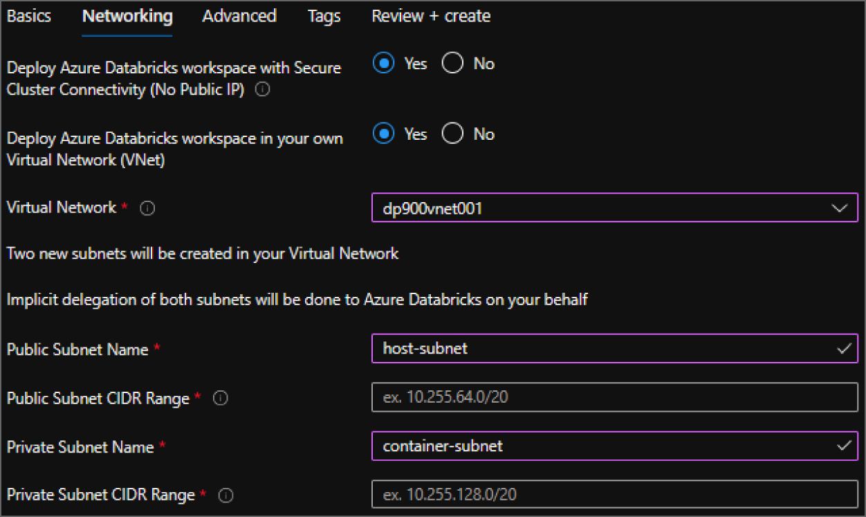
FIGURE 5.6 Create an Azure Databricks workspace: Networking tab.
- The Advanced tab allows you to enable infrastructure encryption to data stored in DBFS. Keep in mind that Azure encrypts storage account data at rest by default, so this option adds a second layer of encryption to the storage account.
- The Tags tab allows you to place tags on the resources deployed with Azure Databricks. Tags are used to categorize resources for cost management purposes.
- Finally, the Review + Create tab allows you to review the configuration choices made during the design process. If you are satisfied with the choices made for Azure Databricks, click the Create button to begin deploying the workspace.
Once the Azure Databricks workspace is deployed, go back to the Azure Databricks page, and click on the newly created workspace. Click on the Launch Workspace button in the middle of the overview page to navigate to the workspace UI and start working within the Databricks ecosystem. Figure 5.7 is an example of what this button looks like.

FIGURE 5.7 Launch Workspace button
A new browser window will open after you click the Launch Workspace button, prompting you to sign in with your Azure AD credentials. Once you are signed in, you will be brought to the Azure Databricks web application where you can begin working with Databricks. The next section describes the key components of the web application.
Navigating the Azure Databricks Workspace UI
The home page for an Azure Databricks workspace serves as a location for users to start working with Databricks. Figure 5.8 is an example of the Azure Databricks web application home page.

FIGURE 5.8 Azure Databricks home page
As you can see in Figure 5.8, there are common task options such as creating a new notebook and importing data. There are also quick navigation links to recently worked on notebooks, Spark documentation, and helpful blog posts.
On the left side of the page is a toolbar with several buttons. The number of buttons in the toolbar varies based on which persona is chosen. Azure Databricks personas include Data Science & Engineering, Machine Learning, and SQL. You can change the persona by clicking the icon below the Databricks logo in the toolbar. Figure 5.9 illustrates this icon and the different options that can be selected from it.
For the purposes of this book and the DP-900 exam, we will only cover the Data Science & Engineering persona. Of the 13 buttons that are under the Data Science & Engineering persona icon, the first 8 buttons are the most relevant to building solutions in Azure Databricks, including the following:
- The Create button opens a pop-up window that allows you to create a new notebook or DBFS table. It also provides quick navigation to pages where you can create a new cluster or a new job.
FIGURE 5.9 Azure Databricks workspace personas
- The Workspace button opens a tab that contains a hierarchical view of the folders and files stored in the workspace. Administrators can use this view to set permissions and import/export folders or files. Usernames act as parent folders (typically Azure AD identities), and users associated with those usernames can add new items to them. Items that users can create from this view include notebooks, libraries, MLflow experiments, and additional subfolders. Figure 5.10 is an example of how the Workspace tab is constructed.

FIGURE 5.10 Azure Databricks Workspace tab
- The Repos button opens a tab that enables developers to create code repositories for their notebooks. Databricks automatically maintains a repository for every user with its native Databricks Repos service. Users can also create shared code repositories for collaborative development efforts. Databricks also supports other Git providers, including GitHub, Bitbucket, GitLab, and Azure DevOps, allowing developers to maintain their code repositories in a single service.
- The Recents button opens a tab that maintains the most recently worked on notebooks.
- The Search button opens a tab that allows users to search for different items in the workspace.
- The Data button opens a hierarchical view of the catalogs, databases, and tables created for each cluster. The metadata for these objects are maintained while a cluster is terminated, allowing developers to easily continue where they left off once the cluster is back online. Depending on how they are defined, tables can be either global or local. Global tables are accessible from any cluster, whereas local tables are only accessible from the cluster they were created from.
- The Clusters button opens the Compute page, displaying the clusters available to the user navigating the workspace. It includes tabs for all-purpose clusters, job clusters, pools, and cluster policies (see Figure 5.11). Users can perform administrative tasks on clusters from this page, such as changing the number and size of cluster nodes and modifying the autoscale setting and changing the inactivity period before clusters are automatically terminated.
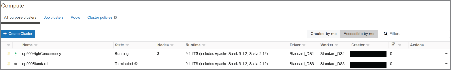
FIGURE 5.11 Azure Databricks Compute page
- The Jobs button opens a page that displays the Spark jobs available to the user navigating the workspace (see Figure 5.12). The Jobs page includes a button that allows users to create new jobs that will execute notebooks on a schedule.

FIGURE 5.12 Azure Databricks Jobs page
Creating a Spark Cluster with Azure Databricks
Spark clusters can be configured and deployed by clicking on the Create Cluster button on the Compute page. Clicking this button will take you to the Create Cluster page, where you will be required to define the following settings (see Figure 5.13):
- Enter a unique cluster name in the Cluster Name field.
- Select a cluster mode from the Cluster Mode field. The options include:
- Standard—Optimized for single-user clusters that run batch or stream processing jobs. This cluster mode supports SQL, Python, R, and Scala workloads.
- High Concurrency—Optimized to run concurrent workloads for users performing interactive analysis. This cluster mode supports SQL, Python, and R workloads.
- Single Node—This cluster mode runs a Spark application on a single compute node. It is recommended for single-user workloads that work with small data volumes.
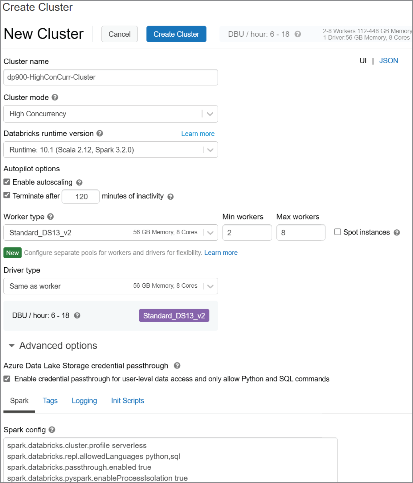
FIGURE 5.13 Azure Databricks Create Cluster page
- Select a Databricks runtime from the Databricks Runtime Version field. This field allows you to select from several Databricks runtimes, including current, older, and beta versions. You can also choose from several Databricks runtimes that are optimized for machine learning workloads.
- The Autopilot Options field allows you to set two settings: autoscaling and auto-terminate. Selecting the Enable Autoscaling check box will configure the cluster to automatically scale between the minimum and maximum number of cluster nodes, based on the workload. You can also enable and set an inactivity threshold (in minutes) after which a cluster will automatically terminate.
- Define the size and number of Azure VMs that will be used as cluster nodes in the Worker Type and Driver Type fields. There are several VM types and sizes to choose from, including those that are optimized for compute-heavy workloads, machine learning applications, and deep learning solutions that require GPUs. If autoscaling is enabled, you will also be able to choose a minimum and maximum number of worker nodes.
- The Advanced Options section allows you to fine-tune your Spark cluster by altering various Spark configuration options, adding libraries or environment-specific settings with init scripts, and defining custom logging. This section also allows you to enable ADLS credential passthrough, which automatically passes the Azure AD credentials of a specific user (when using the Standard or Single Node cluster mode) or the current user (when using the High Concurrency cluster mode) to Databricks for authentication when interacting with an ADLS account.
- Click Create Cluster at the top of the page to begin creating the cluster.
Creating a Notebook and Accessing Azure Storage
The first step to begin working with data is to create a new notebook. You can do this by clicking the Create button on the left-side toolbar and clicking Notebook. This will open a pop-up window that will prompt you to enter a name for the notebook, choose a primary language (Python, Scala, SQL, or R), and select a cluster to attach the notebook to. Once these options are set, click the Create button to create the notebook. You will be guided to the notebook once it is finished being created. Figure 5.14 illustrates how to create a new Python notebook from this window.

FIGURE 5.14 Azure Databricks Create Notebook page
The first cell in a notebook is typically used to import any libraries that will be needed to manipulate data or to establish a connection with an external data source. This section will focus on connecting to Azure Storage, more specifically ADLS. There are three ways to establish a connection to ADLS with Azure Databricks:
- Create a mount point in DBFS to the storage account or the desired folder with an access key, a SAS token, a service principal, or Azure AD credential passthrough.
- Access ADLS via a direct path with a service principal.
- Access ADLS directly with Azure AD credential passthrough.
Creating a service principal is out of scope for the DP-900 exam and will not be covered in this book. Refer to the following blog to learn how to create a service principal that can be used to establish a connection with ADLS: https://docs.microsoft.com/en-us/azure/active-directory/develop/howto-create-service-principal-portal. For now, we will cover how to establish a connection by creating a mount point in DBFS with Azure AD credential passthrough.
To create a mount point in DBFS for an ADLS account, use the dbutils.fs.mount command in the first notebook cell. This command uses three parameters to define a mount point:
- A
sourceparameter that takes the ADLS URI as an argument. If required, the URI can point to a specific subdirectory in ADLS. - A
mount_pointparameter that sets the location (in DBFS) and name of the mount point. - An
extra_configparameter that accepts the authorization information required to access the external storage account. You can set a variable to the OAuth and Spark configuration settings for Azure AD credential passthrough and pass it in theextra_configparameter to make thedbutils.fs.mountcommand reusable and more readable.
Once the mount point has been created, you can run the dbutils.fs.ls command with the mount point name as an argument to verify that you can view the subdirectories in the dp900-adls-container container. See Figure 5.15 for an illustration of both the dbutils.fs.mount and dbutils.fs.ls commands.
Users attempting to read or write data via the mount point will have their credentials evaluated. Alternatively, to creating a mount point, users can access data directly from an ADLS account with Azure AD credential passthrough by passing the ADLS URI in a spark.read command. For example, the following PySpark code assumes that the cluster running the command has Azure AD credential passthrough enabled and the user running the command has the appropriate permissions to the products subdirectory of the dp900-adls-container container:
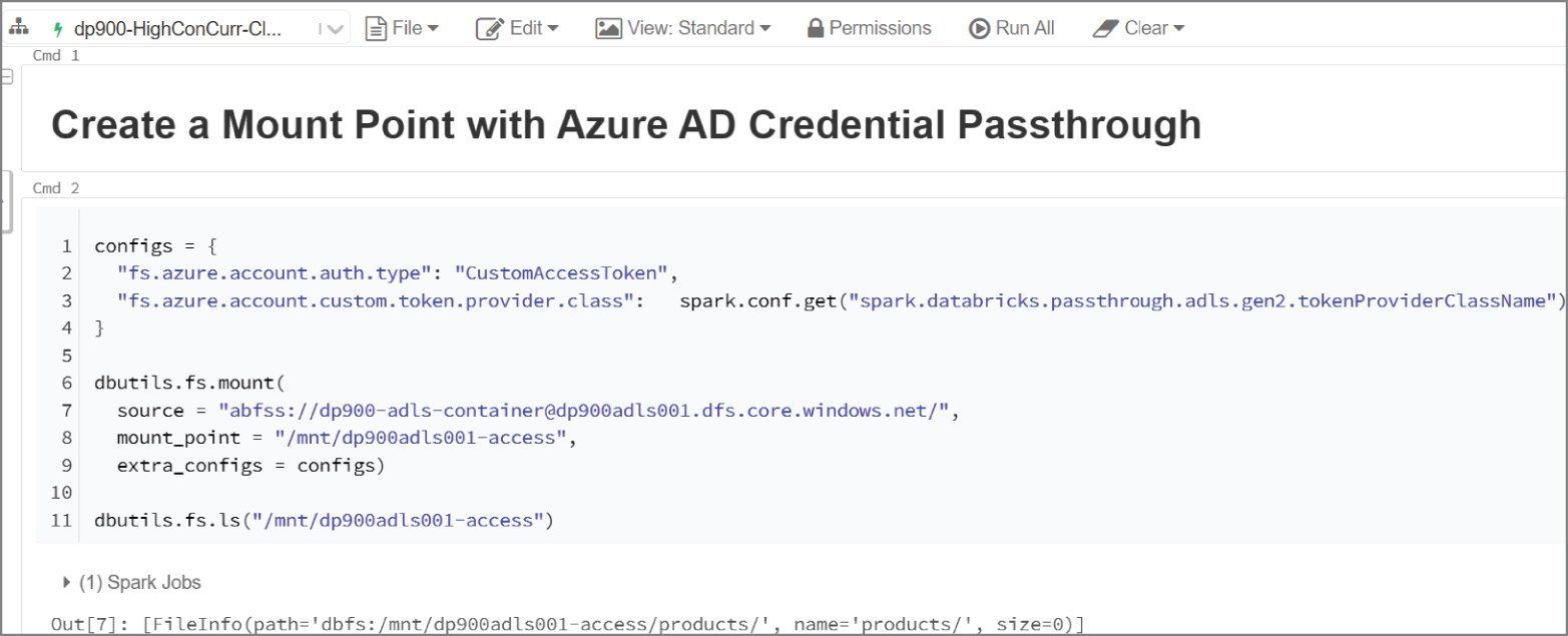
FIGURE 5.15 Creating a mount point with Azure AD credential passthrough
readCsvData = spark.read.csv("abfss://[email protected]/products/products/*.csv")
While Azure AD credential passthrough is the most seamless method for accessing an ADLS account, there are several scenarios where you will need to use one of the other two access methods. For example, batch processing jobs that are orchestrated via ADF or an Azure Databricks job will need to establish a connection to the ADLS path with a service principal to guarantee a consistent connection. Refer to the following to learn more about how to use the different access methods to establish a connection with ADLS: https://cloudblogs.microsoft.com/industry-blog/en-gb/technetuk/2020/07/01/securing-access-to-azure-data-lake-gen-2-from-azure-databricks.
Azure Data Factory
Azure Data Factory (ADF) is a managed cloud service that can be used to build complex ETL, ELT, and data integration projects. With ADF, data engineers can create automated workflows (known as pipelines) that orchestrate data movement and data transformation activities. The following list includes several strengths that make ADF an integral part of any data-driven solution built in Azure:
- The ability to author code-free data pipelines with a graphical user interface (GUI) to simplify pipeline development and maintenance
- Over 90 native connectors for on-premises and multi-cloud data sources that allow for hybrid data movement scenarios
- Integration with several compute services such as Azure HDInsight, Azure Databricks, and Azure SQL to orchestrate transformation activities such as Spark jobs and SQL stored procedures
- Control flow constructs like loops, conditional activities, variables, and parameters that control the customization of a pipeline run
- No-code/low-code data transformations with mapping data flows and Power Query that utilize on-demand Spark clusters for compute
- The ability to trigger pipelines to run at a fixed time, periodic time interval, or in response to an event
- SDK and REST API support that allows developers to manage data factory workflows with existing applications and script languages (such as Azure PowerShell and Azure CLI)
- Native integration with Azure DevOps to incorporate ADF workflows with existing continuous integration/continuous development (CI/CD) pipelines
- The ability to monitor pipeline runs and alert users of any failures
A single Azure subscription can have one or more data factories (also known as ADF instances). This is so users can isolate different projects as well as support different stages of a solution's development life cycle, like development, test, quality assurance, and production.
ADF instances are composed of the following core components:
- Pipelines are a logical grouping of activities that perform data transformation or data movement operations. For example, a pipeline can include a group of activities that move data from external data sources to ADLS followed by an Azure Databricks notebook activity to execute an Azure Databricks notebook that processes the data. Pipeline activities can be chained together to run sequentially, or they can operate independently in parallel.
- Activities represent a data transformation or data movement step in a pipeline. ADF supports the following three types of activities:
- Data movement activities—These activities move data from one source to another. For example, a copy activity can be used to copy data from one data source to another.
- Data transformation activities—These activities perform transformation operations on the data. Some data transformation activities include an Azure Databricks notebook, a Hive query running on an Azure HDInsight cluster, an Azure Function, and an ADF mapping data flow.
- Control activities—These activities control the flow of an ADF pipeline. For example, ADF supports foreach, filter, if, switch, and until activities to control the flow of a pipeline. Developers can also use the Execute Pipeline control activity to run pipelines as a part of another pipeline.
- Linked services define the connection information that is needed for ADF to connect to external resources. ADF supports the following two types of linked services:
- Data store—This linked service type is used to define the connection information for external data sources such as Azure SQL Database, Azure Blob Storage, and Azure Cosmos DB. The full list of supported data stores can be found at
https://docs.microsoft.com/en-us/azure/data-factory/copy-activity-overview#supported-data-stores-and-formats. - Compute resources—This linked service type is used to define the connection information for external compute resources such as Azure HDInsight, Azure Databricks, and Azure Functions. The full list of support external compute stores can be found at
https://docs.microsoft.com/en-us/azure/data-factory/transform-data#external-transformations.
- Data store—This linked service type is used to define the connection information for external data sources such as Azure SQL Database, Azure Blob Storage, and Azure Cosmos DB. The full list of supported data stores can be found at
- Datasets use linked services to represent data structures within data stores, such as a relational database table or a set of files. For example, an Azure Blob Storage–linked service defines the connection information that ADF uses to connect to the Azure Blob Storage account. An Azure Blob Storage dataset can use that linked service to represent a blob container or a specific file within the storage account. Datasets can be used in activities as inputs or outputs.
- Integration runtimes provide the compute infrastructure where activities either run or get triggered from. While the location for an ADF instance is chosen when it is created, integration runtimes can be assigned a different location. This allows developers to run activities with compute infrastructure that is closer to where their data is stored. ADF supports the following three integration runtime types:
- Azure integration runtimes can run data flow activities in Azure, copy activities between cloud data stores, and trigger Azure-based compute activities (such as Azure HDInsight Hive operations or Azure Databricks notebooks). The default AutoResolveIntegrationRuntime that is created with every ADF instance is an Azure integration runtime. Azure integration runtimes support both public and private connections when connecting to data stores and compute services. Private connections can be established by enabling a managed virtual network for the integration runtime.
- Self-hosted integration runtimes are used to run data movement activities between cloud data stores and a data store in a private or on-premises network. This integration runtime type is also used to trigger compute activities that are hosted in on-premises or Azure virtual networks. Self-hosted integration runtimes require that a self-hosted integration runtime client application is installed on one or more machines that are associated with a private or on-premises network and connected to the self-hosted integration runtime in ADF. More information about creating and configuring a self-hosted integration runtime can be found at
https://docs.microsoft.com/en-us/azure/data-factory/create-self-hosted-integration-runtime?tabs=data-factory. - Azure-SSIS integration runtimes are used to execute legacy SQL Server Integration Services (SSIS) packages in ADF. This allows users to lift-and-shift existing SSIS workloads to Azure without having to completely rebuild their control flows and data flows in ADF. When an Azure-SSIS integration runtime is configured, users can leverage it to power an Execute SSIS Package activity. This activity will run the deployed SSIS packages. More information about configuring an Azure-SSIS integration runtime can be found at
https://docs.microsoft.com/en-us/azure/data-factory/concepts-integration-runtime#azure-ssis-integration-runtime.
Now that we have established what the core components of ADF are, let's dive into how to create an ADF instance through the Azure Portal and how to navigate the Azure Data Factory Studio UI.
Deploying an ADF Instance
The following steps describe how to create a new Azure Data Factory instance through the Azure Portal:
- Log into
portal.azure.comand search for Data factories in the search bar at the top of the page. Click Data Factories to go to the Data factories page in the Azure Portal. - Click Create to start choosing the configuration options for your ADF instance.
- The Create Data Factory page includes six tabs to tailor the workspace configuration. Let's start by exploring the options in the Basics tab. Just as with other services, this tab requires you to choose an Azure subscription, a resource group, a name, and a region for the instance. There is an option to choose an older ADF version, but it is recommended to use the most current version. Figure 5.16 is an example of a completed version of this tab.
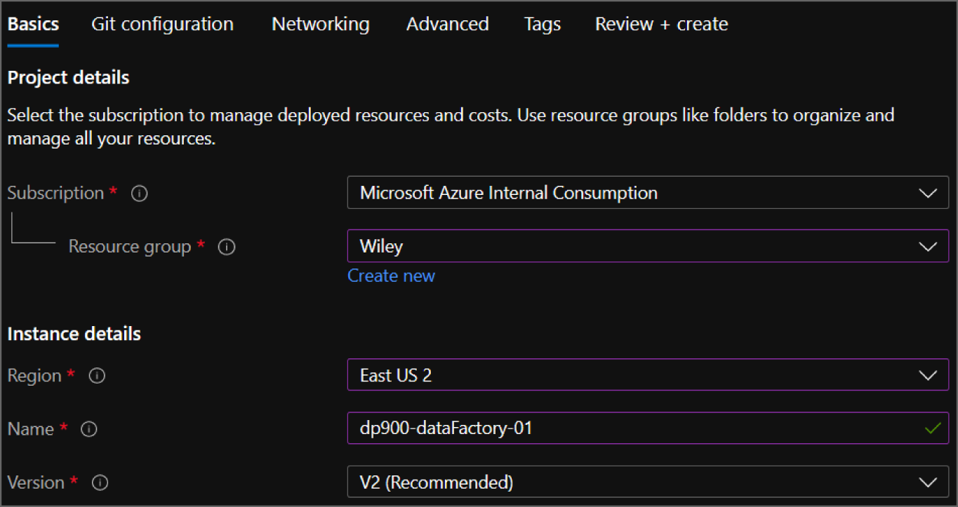
FIGURE 5.16 Create an ADF Instance: Basics tab.
- The Git configuration tab allows you to integrate the ADF instance with an existing Azure DevOps or GitHub repository. ADF entities (such as pipelines, activities, linked services, and datasets) are managed behind the scenes as JSON objects, which can be integrated with existing CI/CD repositories. Click the Configure Git Later check box if you would like to configure a Git pipeline later or save your ADF entities to the data factory service (see Figure 5.17).

FIGURE 5.17 Create an ADF Instance: Git configuration tab.
- The Networking tab allows you to define the networking rules for the auto-resolve integration runtime as well as any self-hosted integration runtimes that you may provision.
- The Advanced tab allows you to supply your own encryption key for blob and file data. Data is encrypted with Microsoft-managed keys by default, but can be changed to a customer-managed key as long as the key is stored in Azure Key Vault.
- The Tags tab allows you to place tags on the ADF instance. Tags are used to categorize resources for cost management purposes.
- Finally, the Review + Create tab allows you to review the configuration choices made during the design process. If you are satisfied with the choices made for the ADF instance, click the Create button to begin deploying the instance.
Once the ADF instance is deployed, go back to the Data factories page and click on the newly created workspace. Click on the Open Azure Data Factory Studio button in the middle of the overview page to navigate to the Azure Data Factory Studio and start working within the ADF ecosystem. Figure 5.18 is an example of the overview page with the Open Azure Data Factory Studio button highlighted.
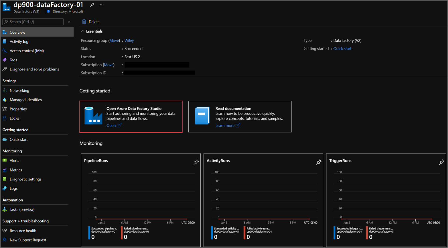
FIGURE 5.18 Azure Data Factory overview page
Clicking the Open Azure Data Factory Studio button will open a new browser window, using your Azure AD credentials to log into the Azure Data Factory Studio. Figure 5.19 highlights the main features of the Azure Data Factory Studio home page.

FIGURE 5.19 Azure Data Factory Studio home page
Navigating the Azure Data Factory Studio
The Azure Data Factory Studio is the central tool for authoring ADF resources. There are several buttons on the home page that enable users to start building new workflows very quickly:
- The Ingest button, which navigates users to the Copy Data tool. This tool allows developers to quickly begin copying data from one data store to another
- The Orchestrate button, which navigates users to the Author page where they can begin building pipelines
- The Transform Data button, which opens a new page where developers can build a mapping data flow
- The Configure SSIS button, which navigates users to a new page where they can configure a new Azure-SSIS integration runtime
On the left side of the page there is a toolbar with four buttons, including a Home button that will navigate users back to the Azure Data Factory Studio home page. The following list describes how you can use the other buttons in the toolbar to build and manage ADF resources:
- The Author button opens the Author page where users can build and manage pipelines, datasets, mapping data flows, and Power Query activities. Figure 5.20 is an example of the Author page with a single activity pipeline that copies data from Azure SQL Database to ADLS.
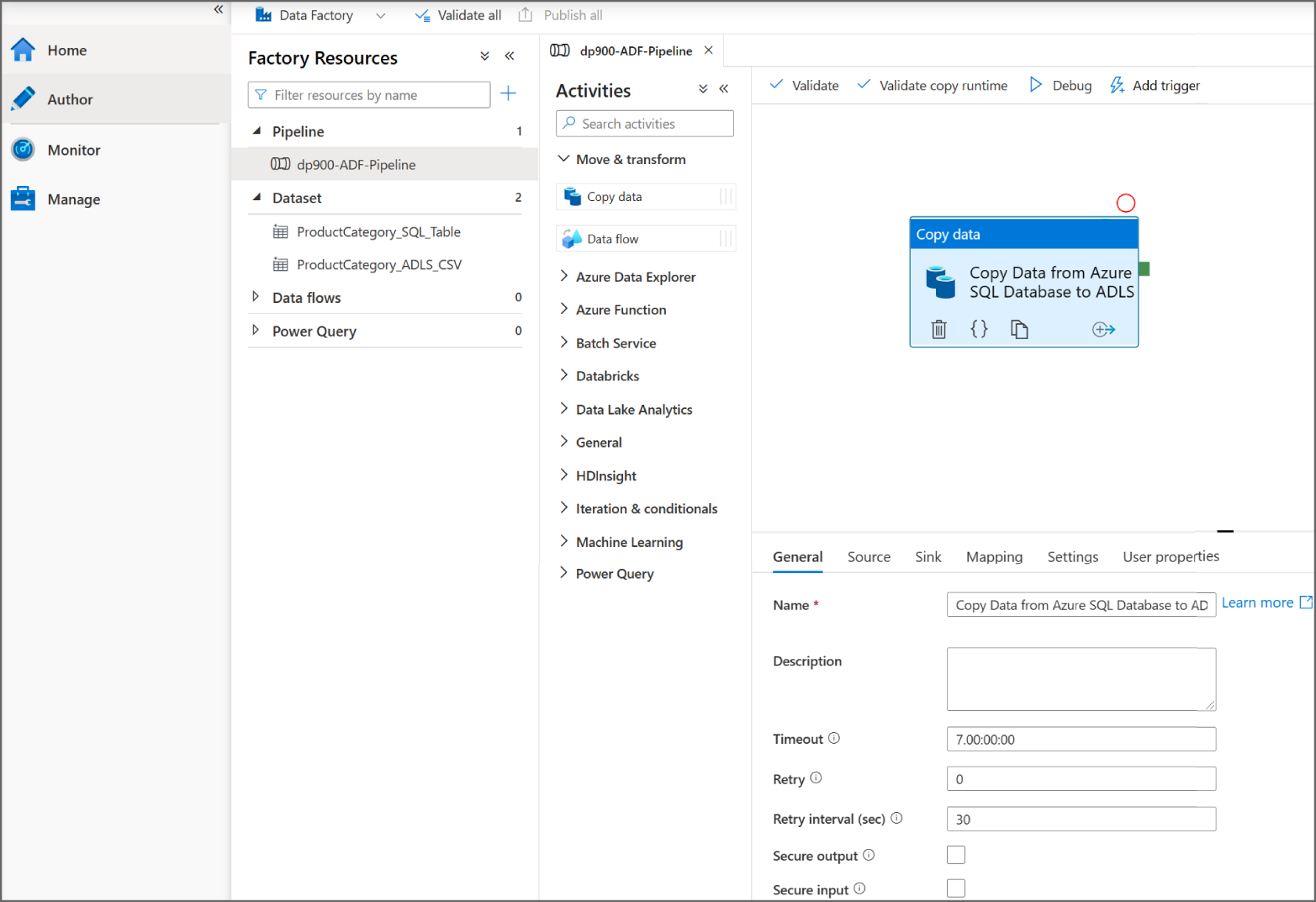
FIGURE 5.20 Azure Data Factory Studio Author page
- The Monitor button opens a page that provides performance metrics for pipeline runs, trigger runs, and integration runtimes. Figure 5.21 is an example of the Monitor page.
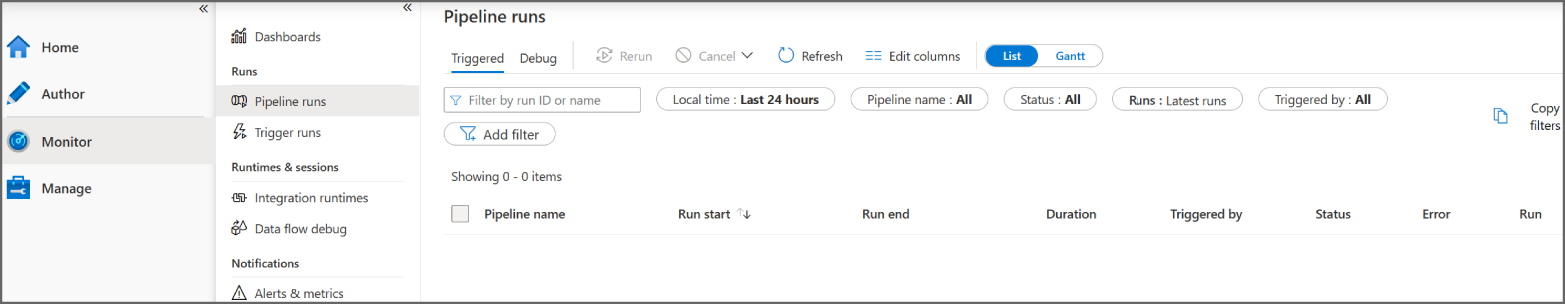
FIGURE 5.21 Azure Data Factory Studio Monitor page
- The Manage button opens a page (see Figure 5.22) that allows you to perform several management tasks, such as those listed here:
- Create or delete linked services.
- Create or delete integration runtimes.
- Link an Azure Purview account to catalog metadata and data lineage.
- Connect the ADF instance to a Git repository.
- Create or delete pipeline triggers.
- Configure a customer managed encryption key and define access management for the ADF instance.

FIGURE 5.22 Azure Data Factory Studio Manage page
The following section, “Building an ADF Pipeline with a Copy Data Activity,” will detail how to create the activity, datasets, and linked services that are associated with the pipeline in Figure 5.20 (shown earlier). More specifically, it will demonstrate how to use the copy activity to copy data from an Azure SQL Database to an ADLS account. The source database is restored from the publicly available AdventureWorksLT2019 database backup. If you would like to build this demo on your own, you can find the database backup at https://docs.microsoft.com/en-us/sql/samples/adventureworks-install-configure?view=sql-server-ver15&tabs=ssms#download-backup-files.
Building an ADF Pipeline with a Copy Data Activity
The first step in creating an ADF pipeline through the Azure Data Factory Studio is to navigate to the Author page by clicking either the Author button on the left-side toolbar or the Orchestrate button on the home page. The left pane on the Author page contains a tree view named Factory Resources. From here, you can create or navigate through existing pipelines, datasets, mapping data flows, or Power Query activities by clicking the + button or the ellipsis (…) next to each menu item. Figure 5.23 illustrates how to create a blank pipeline by clicking the + button.
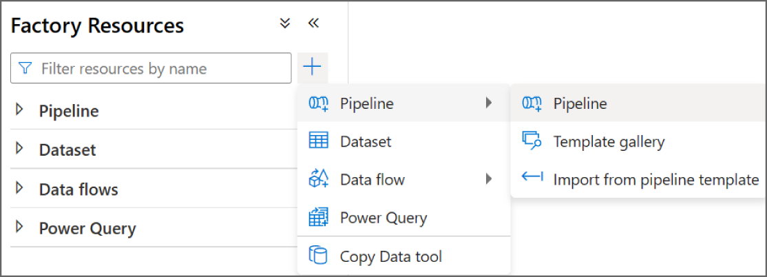
FIGURE 5.23 Creating a blank ADF pipeline
After you click Pipeline, a blank pipeline canvas will open with a new toolbar on the left side of the canvas that contains every activity that can be added to the pipeline. Any of these activities can be dragged from the Activities toolbar and dropped onto the central canvas to build out the pipeline. At the top of the canvas there are buttons to validate the pipeline for any errors, debug the pipeline, and add a trigger to the pipeline. On the right side of the canvas is the Properties tab where you can add a friendly name and a description for the pipeline. At the bottom of the canvas there are options to create new parameters and variables that can make pipeline runs more dynamic. Figure 5.24 illustrates each of these components with a friendly name added in the Properties tab.

FIGURE 5.24 The ADF Pipeline Creation page
To add a copy activity, expand the Move & Transform option in the Activities toolbar and drag the Copy Data activity to the canvas. The new activity will include six configuration tabs that will be located at the bottom of the tab. The first tab (General tab) allows you to provide a friendly name and description for the activity as well as time-out and retry settings. Figure 5.25 is an example of this view with a friendly name that describes the activity's functionality.

FIGURE 5.25 Copy Data Activity: General tab
Out of the six copy activity configuration tabs, only two of them require user input: the Source tab and the Sink tab. These two tabs will define the source dataset and the destination, or sink, dataset that the data is being copied to. The Source tab allows you to choose an existing dataset or create a new one. If you click the + New button, a new page will open where you can choose from one of the available data source connectors (see Figure 5.26).

FIGURE 5.26 New Dataset page
In the search bar, type Azure SQL Database and choose the Azure SQL Database connector. Click Continue at the bottom of the page to open the Set Properties page for the dataset. This page allows you to set a friendly name for the dataset and choose/create the linked service that will be used to connect to the data source. Expand the Linked Service drop-down menu and click + New to create a linked service for the database. This will open a new page where you can set a friendly name for the linked service, the integration runtime, and the connection information for the database. Figure 5.27 is a completed example of the New Linked Service page for an Azure SQL Database.
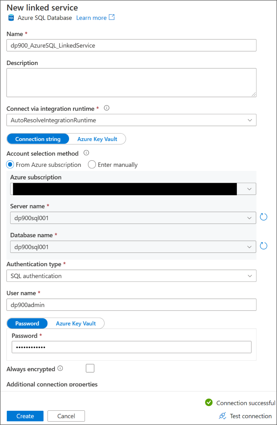
FIGURE 5.27 New linked service page: Azure SQL Database
Once the settings for the linked service are properly set, click the Create button to create the linked service and to be redirected to the Set Properties page for the dataset. With the linked service defined, the next step will be to either choose the table or view that the dataset will represent or leave the Table Name setting blank. For the purposes of this example, we will choose the SalesLT.ProductCategory table. Figure 5.28 is a completed example of the Set properties page.

FIGURE 5.28 Set properties page for a new dataset: Azure SQL Database
After you click OK at the bottom of the Set Properties page, the dataset will be created and added as the source dataset in the copy activity. Because the source dataset is an Azure SQL Database, the Source tab includes several optional settings that are tailored to relational databases. For example, if you did not choose a table or view in the dataset tab, you can use a query or a stored procedure to define the dataset. You can also parameterize this setting so that the dataset varies based on the value passed to the parameter. Figure 5.29 illustrates the list of options that are available in the Source tab for an Azure SQL Database.

FIGURE 5.29 Copy Data Activity: Source tab
Now that the source dataset is set, the next step is to configure a sink dataset. The Sink tab provides the same options as the Source tab, along with the ability to create a new dataset. Because this example uses an ADLS account as the sink data store, choose the Azure Data Lake Storage Gen2 connector on the New Dataset page. After clicking Continue, you will be prompted to set a file format for the dataset. For this example, choose the DelimitedText (CSV) option and click Continue.
As with the Azure SQL Database dataset, the Set Properties page allows you to set a friendly name for the dataset and choose/create the linked service that will be used to connect to the data source. The new linked service page for ADLS is also similar to the new linked service page for Azure SQL Database as it allows you to set a friendly name for the linked service, the integration runtime, and the connection information for the storage account (see Figure 5.30). Click the Create button to create the linked service and to be redirected to the Set Properties page for the dataset.

FIGURE 5.30 New linked service page: ADLS
With the ADLS linked service defined, the Set Properties page allows you to either set a file path for the dataset or leave it blank. This example uses the dp900-adls-container/products/ file path for the sink dataset (see Figure 5.31).

FIGURE 5.31 Set properties page for a new dataset: ADLS
After you click OK at the bottom of the Set Properties page, the dataset will be created and added as the sink dataset in the copy activity. Like the Azure SQL Database dataset, there are several additional settings in the Sink tab that will be relevant to the chosen dataset type. The Sink tab (and the Source tab) also allows you to open the dataset with the Open button (next to the Sink dataset setting). This button opens a new page that allows you to make several changes that are specific to the dataset type. Because the sink dataset is CSV data stored in ADLS, the list of settings that can be edited include how the data is compressed, the column and row delimiters for the data, how the data is encoded, and whether the first row should be treated as a header. You can also use this page to define a filename for the dataset. Figure 5.32 illustrates this page with all of the available dataset settings.
Once the dataset settings are properly configured, navigate back to the pipeline by clicking on the pipeline tab at the top of the page. Click on the Mapping tab to map the source dataset columns to the sink columns. This tab also allows you to set datatype settings, such as the date/time format, and whether to truncate data that is longer than what the column definition allows. Figure 5.33 is an example of the Mapping tab.
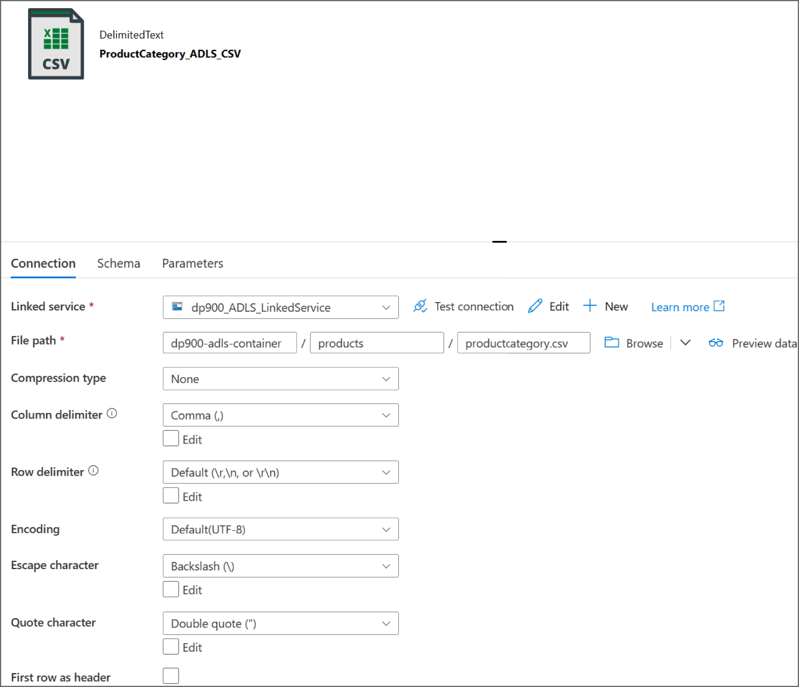
FIGURE 5.32 Using the Azure Data Factory Studio to edit a CSV dataset
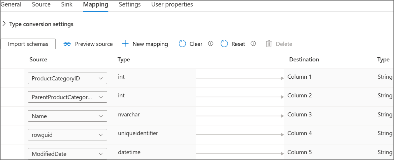
FIGURE 5.33 Copy Data Activity: Mapping tab
Navigate to the Settings tab after mapping the source and sink columns. This tab allows you to set how many DIUs you want allocated to the pipeline, or if you want the pipeline to automatically apply the optimal number of DIUs. You can also set the degree of parallelism that the copy activity will use if the volume of source dataset requires a scale-out solution.
The last tab in the copy activity Is the User Properties tab. This allows you to tag and monitor specific ADF resources, such as datasets.
Click the Publish All button at the top of the page to save the pipeline and the datasets. To run the pipeline or schedule the pipeline to run at a later time, click the Add Trigger button at the top of the canvas and choose either Trigger now to begin a pipeline run or New/Edit to create a scheduled or event-based trigger. Figure 5.34 illustrates where the Publish All and Add Trigger buttons are located. Once the pipeline is published, click the Trigger button to either run it right then and there or to create a schedule to run it at a later time.
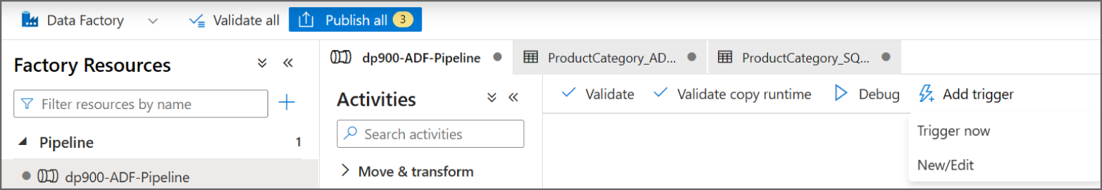
FIGURE 5.34 Using the Publish all button to save the pipeline and datasets.
Real-Time Azure Data Processing Services
While the previously described set of services can be used in a variety of data processing tasks, it is important to note that there are other Azure data services that are used for niche data processing use cases. For example, Azure Stream Analytics and Azure Data Explorer are almost exclusively used in stream processing workflows. These services are out of scope for the DP-900 exam and will only be covered briefly in the following sections.
Azure Stream Analytics
Azure Stream Analytics is a PaaS stream processing engine that can be used to process high volumes of streaming data from multiple sources. Users can create Azure Stream Analytics jobs through the Azure Portal, Azure CLI, Azure PowerShell, or an Infrastructure as Code template like ARM. Jobs consist of three core components: one or more inputs, a query, and one or more outputs.
Inputs can include real-time message ingestion services like Azure Event Hubs and Azure IoT Hub as well as persistent data stores like Azure Blob Storage and Azure SQL Database. This enables developers to combine streaming data with historical data or with reference data for lookup operations.
Developers can use the Stream Analytics query language to filter, sort, aggregate, or join data from different sources. This language is a subset of standard T-SQL with additional functionality to apply computations over specific time windows. The language can also be extended with JavaScript and C# user-defined functions.
Jobs deliver processed information to one or more outputs. Azure Stream Analytics allows you to customize what happens based on the results of the data that was processed. Here are some common outputs:
- Services like Azure Event Hubs, Azure Service Bus, or Azure Functions to trigger alerts or custom workflows
- Power BI dashboards for real-time dashboarding
- Persistent data stores like Azure Blob Storage, ADLS, Azure SQL Database, or Azure Synapse Analytics dedicated SQL pools for long-term storage or batch processing
If you would like to learn more about Azure Stream Analytics, visit https://docs.microsoft.com/en-us/azure/stream-analytics/stream-analytics-introduction.
Azure Data Explorer
Azure Data Explorer is a near real-time processing engine that analyzes structured, semi-structured, and unstructured data across time windows. It uses the Kusto Query Language (KQL) to analyze data and is capable of ingesting and analyzing petabytes of data. Typical use cases for Azure Data Explorer include interactively analyzing logs and conducting time series analytics on metric data from IoT sensors.
If you would like to learn more about Azure Data Explorer, visit https://docs.microsoft.com/en-us/azure/data-explorer/data-explorer-overview.
End-to-End Analytics with Azure Synapse Analytics
Azure Synapse Analytics is an enterprise analytics system that integrates multiple services that serve analytical workloads in a single environment. Through the Azure Synapse workspace, users can leverage the following services to build a modern data warehouse solution:
- Synapse Studio is a unified environment where users can manage all components of the Azure Synapse Analytics ecosystem. The following tasks can be performed with Synapse Studio:
- Build ETL and ELT workflows that can be automated to run at predetermined times or after specific events.
- Configure and deploy dedicated SQL, Apache Spark, and Data Explorer pools.
- Develop SQL, Spark, or KQL code to analyze data with SQL, Spark, or Data Explorer pools.
- Monitor resource utilization, query performance, and user access across SQL, Spark, or Data Explorer pools.
- Integrate with CI/CD and data catalog services such as Azure DevOps and Azure Purview.
- Dedicated SQL pools are analytical data stores that use a scale-out, massively parallel processing (MPP) architecture to effectively manage several petabytes of data. Storage and compute are decoupled, allowing users to easily scale compute power without having to move data. Azure Synapse workspaces can have one or more dedicated SQL pools.
- Serverless SQL pool is a serverless query service that allows analysts to use T-SQL to interactively query Azure Storage files. It does not have local storage or ingestion capabilities. Every Azure Synapse workspace comes with a serverless SQL pool endpoint that cannot be deleted. Azure Synapse workspaces only support a single serverless SQL pool (named “Built-in”).
- Apache Spark pools are managed, open-source Apache Spark clusters in the Azure Synapse ecosystem. Users can set the number of compute nodes in a cluster, with an option to automatically scale clusters up and down based on the workload. Cluster nodes can be configured with predefined node sizes, ranging from small (4 vCores, 32 GB of memory) to xxx large (80 vCores, 504 GB of memory). With Synapse notebooks, data engineers can use an Apache Spark pool to analyze data with Python, SQL, R, Scala, Java, or .NET code. More information about Azure Synapse Analytics Apache Spark pools can be found at
https://docs.microsoft.com/en-us/azure/synapse-analytics/spark/apache-spark-pool-configurations. - Synapse pipelines are orchestration workflows that define a set of actions to perform on data. This service has the same functionality as ADF but is available through the Azure Synapse workspace, making it more ideal for users who want to manage their analytical data stores, data engineering activities, and orchestration pipelines from the same environment. The concepts covered previously in this chapter for ADF also apply to Azure Synapse pipelines.
- Synapse Link is a hybrid transactional and analytical processing (HTAP) tool that enables users to run near real-time analytical queries over transactional data. With Azure Synapse Link, users do not need to build complex ETL workflows that move data from a transactional data store to an analytical one. Instead, Synapse Link synchronizes data from transactional data stores like Azure Cosmos DB and Azure SQL Database with a column-oriented analytical data store that can be explored with the Azure Synapse Analytics serverless SQL pool or an Azure Synapse Analytics Apache Spark pool. More information about Azure Synapse Link can be found at
https://docs.microsoft.com/en-us/azure/cosmos-db/synapse-link. - Data Explorer pools are optimized for telemetry analytics. Azure Synapse data explorer automatically indexes free-text and semi-structured data that is found in telemetry data, such as logs and time series data. The concepts covered previously in this chapter for Azure Data Explorer also apply to Azure Synapse data explorer.
- Power BI is a reporting service that can be used to develop dashboards, reports, and datasets for self-service BI. Azure Synapse Analytics allows users to connect a Power BI workspace to an Azure Synapse Analytics workspace for a seamless development experience. This provides analysts with a single environment for analyzing data, developing insightful reports, and sharing the reports to various business users. Power BI workspaces will be described in further detail in Chapter 6, “Reporting with Power BI.”
As you can see, Azure Synapse Analytics allows users to leverage several different technologies to build modern data warehouse solutions in the same environment. The following sections describe how to get started with Azure Synapse Analytics, including how to deploy a workspace and how to navigate Synapse Studio. Afterward, we will examine the two categories of SQL pools, dedicated and serverless, and when to use them.
Deploying an Azure Synapse Analytics Workspace
Like any service in Azure, an Azure Synapse workspace can be deployed though the Azure Portal, Azure PowerShell, or Azure CLI or via an Infrastructure as Code template. The following steps describe how to deploy a new Azure Synapse workspace through the Azure Portal:
- Log into
portal.azure.comand search for Azure Synapse Analytics in the search bar at the top of the page. Click Azure Synapse Analytics to go to the Azure Synapse Analytics page in the Azure Portal. - Click Create to start choosing the configuration options for your Azure Synapse workspace.
The Create Synapse Workspace page includes five tabs to tailor the workspace configuration. Let's start by exploring the options in the Basics tab. Just as with other services, this tab requires you to choose an Azure subscription, a resource group, a name, and a region for the workspace. You will also need to associate an ADLS account to the workspace. Azure Synapse will use this ADLS account as the primary storage account and the container to store workspace data. A completed example of this tab can be seen in Figure 5.35.
The Security tab requires you to create an administrator account for the serverless and dedicated SQL pools managed by the workspace. You can also use this tab to enable network access to the associated ADLS account with the workspace managed identity and enable double encryption with a key that you provide. Figure 5.36 is an example of the security tab.
The Networking tab allows you to choose whether to set up a dedicated, managed VNet for Azure Synapse Analytics. You can also enable access for all IP addresses through this tab or choose to grant access to specific IP addresses after the workspace is deployed.
The Tags tab allows you to place tags on the resources deployed with Azure Synapse Analytics. Tags are used to categorize resources for cost management purposes.
Finally, the Review + Create tab allows you to review the configuration choices made during the design process. If you are satisfied with the choices made for the Azure Synapse Analytics workspace, click the Create button to begin deploying the workspace.
Once the Azure Synapse Analytics workspace is deployed, go back to the Azure Synapse Analytics page, and click on the newly created workspace. From the Azure Portal, administrators can set Azure AD authentication, create new analytics pools (dedicated SQL, Apache Spark, and Data Explorer pools), configure network settings, and monitor performance. Click on the Open Synapse Studio button in the middle of the overview page to navigate to Synapse Studio UI. Figure 5.37 is an example of the workspace overview page with the Open Synapse Studio button highlighted.

FIGURE 5.35 Create an Azure Synapse Analytics workspace: Basics tab.
A new browser window will open after you click the Open Synapse Studio button, using your Azure AD credentials to log in to the workspace. Figure 5.38 is an example of the Synapse Studio home page.
Navigating the Synapse Studio UI
Synapse Studio is the central tool for administering and managing all aspects of the Azure Synapse Analytics ecosystem that enable users to start building new Azure Synapse Analytics workflows very quickly, including an Ingest button to begin moving data, an Explore and Analyze button to navigate users to Azure Synapse Analytics tutorials, and a Visualize button to connect to a Power BI workspace. On the left side of the page there is a toolbar with six buttons, including a Home button that will navigate users back to Synapse Studio home page. The following list describes how you can use the other buttons in the toolbar to build a modern data warehouse:

FIGURE 5.36 Create an Azure Synapse Analytics workspace: Security tab.

FIGURE 5.37 Azure Synapse workspace overview page

FIGURE 5.38 Synapse Studio home page
- The Data button opens a page that allows you to link external and integrated datasets to the Azure Synapse Analytics workspace. It has two tabs, the Workspace tab to organize any analytics pools that are associated with the workspace and the Linked tab to organize external storage such as ADLS or Azure Blob Storage. From this page, you can create new blank script pages or predefined scripts that run bulk load operations or select the top 100 rows of a table. Figure 5.39 is an example of the Workspace tab and the external data source options that can be added by clicking the + button.
- The Develop button opens a page that organizes all SQL scripts, KQL scripts, notebooks, mapping data flows, and Apache Spark jobs. Figure 5.40 is an example of the Develop page and the various objects that can be added by clicking the + button.
- The Integrate button opens a page that allows you to build data orchestration and movement pipelines. You can create new pipelines or use the Copy Data tool to perform a one-time or scheduled data load from over 90 data sources. The functionality is similar to ADF, with some additional activities that are specific to Azure Synapse Analytics. Figure 5.41 is an example of the Integrate page and the Synapse-specific activities.

FIGURE 5.39 Synapse Studio Data page
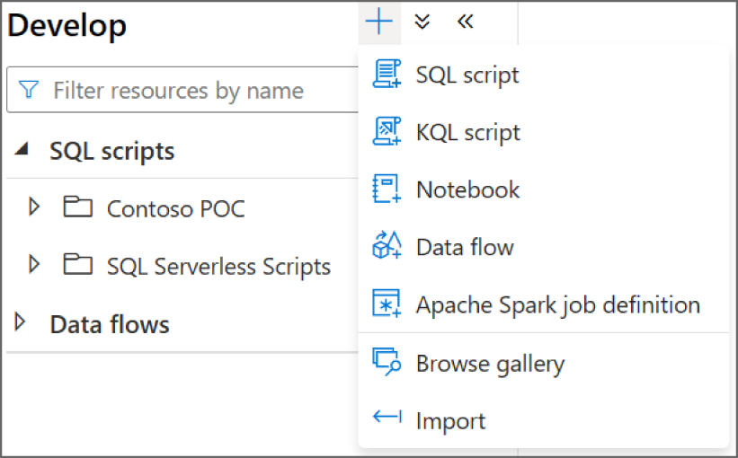
FIGURE 5.40 Synapse Studio Develop page
- The Monitor button opens a page that provides a comprehensive view of the performance details and statuses for the different analytics pools, activities, and integration pipelines. Figure 5.42 is an example of the Monitor page with a focus on the SQL pools section.
- The Manage button opens the Manage page (see Figure 5.43). This page allows you to perform several management tasks:
- Create, configure, pause, and resume analytics pools.
- Create and delete linked services. Linked services provide the connection information to external data sources that are used in Synapse pipelines.
- Link an Azure Purview account to catalog metadata and data lineage.
- Create and delete triggers. A trigger is used to automate when a Synapse pipeline is executed. Types of triggers include schedules, storage events, and custom events.
- Create and delete integration runtimes. An integration runtime (IR) is the compute infrastructure used by Synapse pipelines.
- Manage all security access controls and credentials.
- Link a Git repository to your Azure Synapse Analytics workspace.

FIGURE 5.41 Synapse Studio Integrate page
Dedicated SQL Pools
Azure Synapse Analytics dedicated SQL pools (formerly Azure SQL Data Warehouse) are relational data stores that use a massively parallel processing (MPP) architecture to optimally manage large datasets. This can be done by separating compute and storage by using a SQL engine to perform computations and Azure Storage to store the data. Dedicated SQL pools use a relational schema, typically a star schema, to serve data to users as tables or views for business intelligence applications.

FIGURE 5.42 Synapse Studio Monitor page
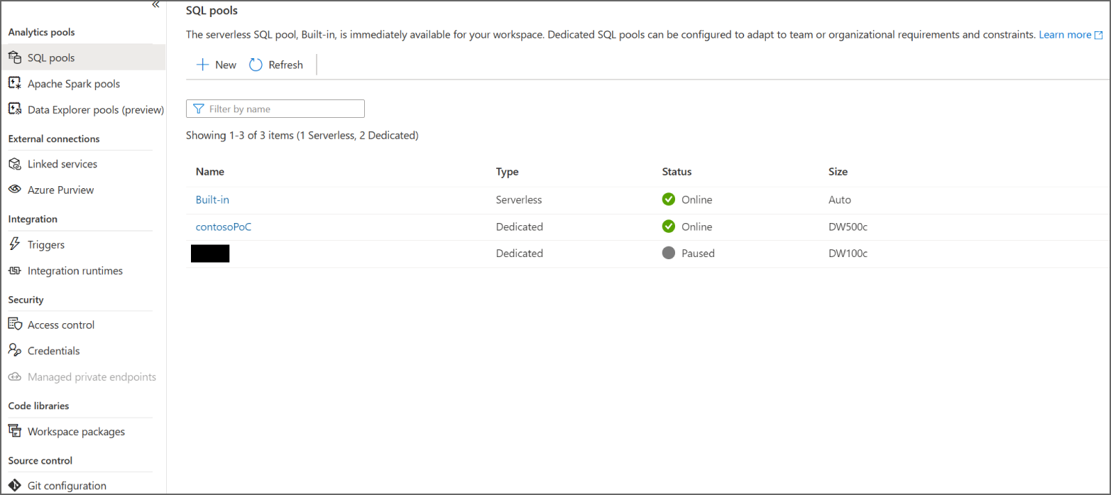
FIGURE 5.43 Synapse Studio Manage page
In a modern data warehouse architecture, a dedicated SQL pool is at the end of an ETL/ELT process, serving as the single source of truth for data analysts and BI applications. Tables using columnstore compression can store an unlimited amount of data, making dedicated SQL pools the ideal destination data store for big data workloads that process several terabytes or even petabytes worth of data. Additional processes can also extract subsets of data that represent specific business segments from a dedicated SQL pool and load them into Azure Analysis Services or Power BI OLAP models for self-service BI scenarios.
As mentioned in Chapter 2, dedicated SQL pools shard data into 60 distributions across one or more compute nodes depending on the dedicated SQL pool's service level objective (SLO). Tables can be defined with one of three distribution patterns to optimize how data is sharded throughout the distributions. The following list is a quick reminder of the three distribution patterns and when to use each one:
- Hash distribution uses a hash function to deterministically assign each row to a distribution. When defining a table with this distribution type, one of the columns is designated as the distribution column. This distribution type offers the most optimal query performance for joins and aggregations on large tables. For this reason, large fact tables are typically defined as hash distributed tables. However, keep in mind that the values of a column designated as the distribution column cannot be updated. The column must also have a high number of unique values and a low number of null values. Poorly chosen distribution columns can lead to unacceptable query response times that cannot be resolved without re-creating the table. Use round robin distribution instead of hash distribution if there are no suitable distribution columns for a large fact table.
- Round robin distribution evenly and randomly distributes rows across all 60 distributions. Staging tables and fact tables without a good distribution column candidate are typically defined as round robin tables.
- Replicated tables cache a full copy of a table on the first distribution of each compute node. This removes the need to shuffle data when querying data from multiple distributions. However, replicated tables can require extra storage, making them impractical for large tables or tables that are frequently written to. For this reason, only small tables (less than 2 GB) or tables that store static data (such as reference data) are defined as replicated tables.
Along with classic relational database features such as partitioning, row-store indexes, and statistics, dedicated SQL pools include several features that optimize the performance of analytical queries that aggregate large numbers of rows. These features are especially useful for querying historical data from fact tables, which can quickly become very large. Some of the most important features are as follows:
- Clustered columnstore indexes (CCIs) physically organize tables into a columnstore format. With a columnstore format, rows of data are compressed into rowgroups, optimizing how large tables are stored (up to 10X data compression versus uncompressed data) and the processing time for queries that perform table scans (up to 10X times the query performance over traditional row-oriented indexes). This is ideal for data warehouses, especially for large fact tables that are subject to analytical queries that scan large amounts of data.
- Materialized views are virtual tables created from a SELECT statement and presented to users as logical tables. Like a standard view, a materialized view abstracts the complexity of the underlying SELECT statement from users so that there is no need to rewrite the statement. Unlike a standard view, materialized views precompute, store, and maintain data in a dedicated SQL pool just like a table. Because recomputation is not needed each time a materialized view is used, queries running against a materialized view are much faster than a standard view. Materialized views improve the performance of complex queries with several joins and aggregations while simplifying query maintenance. The query optimizer in a dedicated SQL pool can also use a materialized view to improve a query's execution plan without the query needing to make a direct reference to the materialized view. Queries used to build a materialized view must include an aggregation in its definition.
- Result set caching improves query performance by automatically caching query results in a dedicated SQL pool user database for later use. This allows subsequent runs of the query to get results directly from the cache instead of recomputing the results. Result set caching can be enabled for a database by running the following T-SQL command:
ALTER DATABASE dp900dedicatedSQLpoolSET RESULT_SET_CACHING ON;
Unlike OLTP database engines like Azure SQL Database, dedicated SQL pools are not suitable for transactional workloads, which are characterized by frequent, small write operations and queries that interact with only a few rows of data (such as a query with a WHERE clause that performs a seek operation to a specific set of rows). Instead, it is best used for bulk write operations and queries that perform aggregations over large amounts of data.
In addition to Synapse Studio, dedicated SQL pools support several management tasks and tools that are commonly used by other Microsoft SQL offerings (such as SQL Server and Azure SQL Database). SQL developers can connect to a dedicated SQL pool with Azure Data Studio or SQL Server Management Studio (SSMS). Database administrators can also leverage security postures that are common to Azure SQL, such as the following:
- Network isolation with an Azure VNet or an IP firewall
- Access management with SQL authentication and Azure AD
- Data encryption and obfuscation with TDE and TLS, Always Encrypted, row-level encryption, column-level encryption, and dynamic data masking
- Security management with the SQL Vulnerability Assessment and Advanced Threat Protection services
More information about the different security components available for Azure SQL can be found in Chapter 2.
Deploying and Scaling a Dedicated SQL Pool
In addition to the methods described previously in this book for deploying Azure resources, users can deploy a new dedicated SQL pool through Synapse Studio with the following steps:
- Click on the Manage button on the left-side toolbar in Synapse Studio and click on SQL pools. Click + New to begin creating a new dedicated SQL pool. You can see an example of the SQL pools page in Figure 5.43 (shown earlier).
- The New dedicated SQL pool page includes four tabs to tailor the workspace configuration. Let's explore the options in the four tabs.
- The Basics tab requires that you set a name and an initial performance level (SLO) for the dedicated SQL pool. The performance level can be set by dragging the scale to the left or to the right. Figure 5.44 is a completed example of the Basics tab.
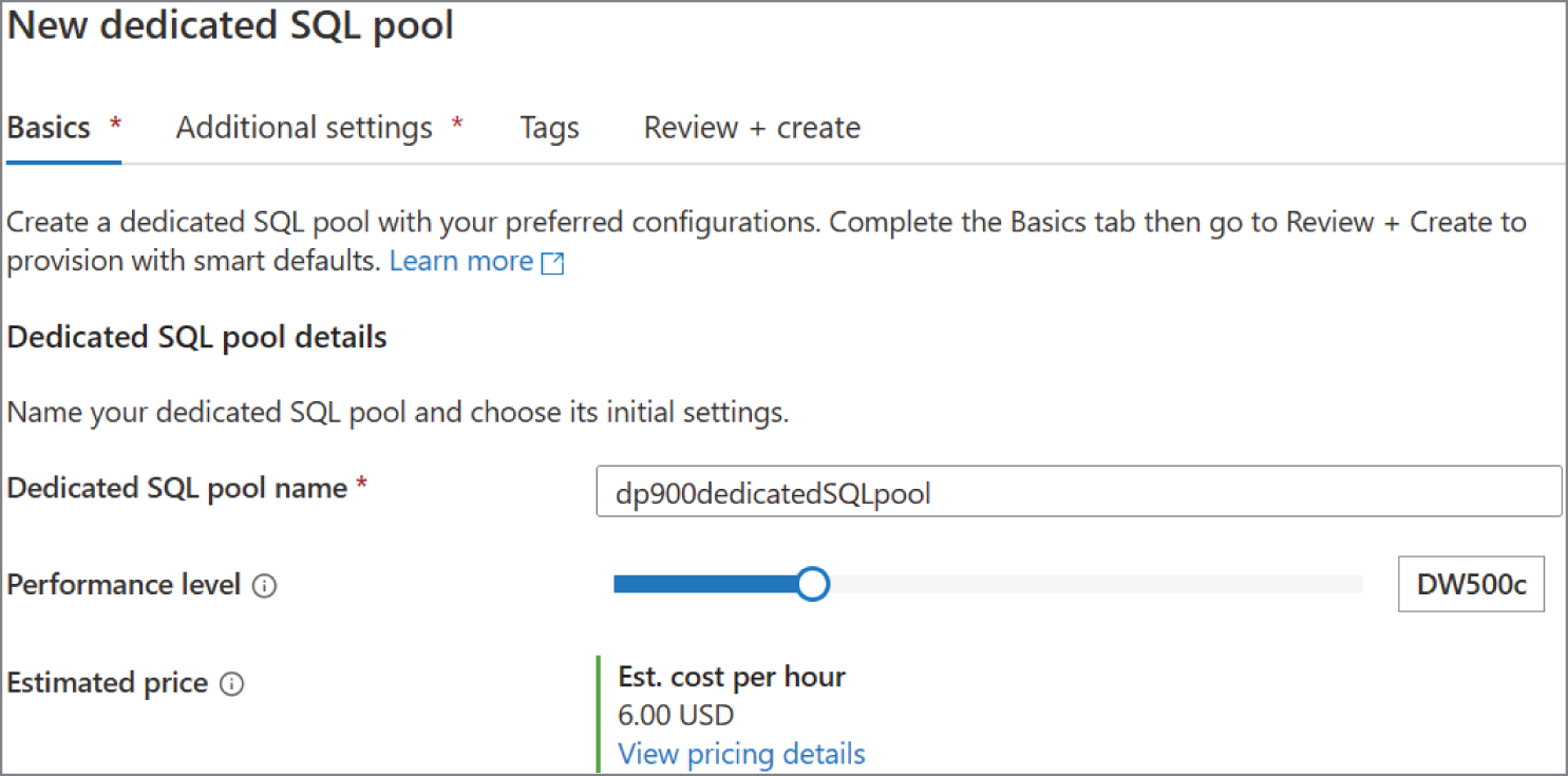
FIGURE 5.44 New dedicated SQL pool: Basics tab
- The Additional settings tab allows you to set the initial state of the dedicated SQL pool, including whether to start with a blank database or from a database backup. Figure 5.45 is a completed example of the Additional settings tab.

FIGURE 5.45 New dedicated SQL pool: Additional settings tab
- The Tags tab allows you to place a tag on the dedicated SQL pool. Tags are used to categorize resources for cost management purposes.
- Finally, the Review + Create tab allows you to review the configuration choices made during the design process.
- The Basics tab requires that you set a name and an initial performance level (SLO) for the dedicated SQL pool. The performance level can be set by dragging the scale to the left or to the right. Figure 5.44 is a completed example of the Basics tab.
- If you are satisfied with the choices made for the dedicated SQL pool, click the Create button on the Review + Create tab to begin deploying the new dedicated SQL pool.
As with any PaaS database in Azure, the SLO of a dedicated SQL pool can be easily scaled up or down to meet different workload needs. This can be done through the Azure Portal, Azure PowerShell, T-SQL, or the Create or Update Database REST API. The following is a sample T-SQL script that updates a dedicated SQL pool's SLO to DW1000c:
ALTER DATABASE dp900dedicatedSQLpoolMODIFY (SERVICE_OBJECTIVE = 'DW1000C');
Because compute and storage are separated, dedicated SQL pools can be paused when they are not used to save on compute costs. Users can pause and restart dedicated SQL pools through the Azure Portal, Synapse Studio, Azure PowerShell, and the dedicated SQL pool REST APIs. Pause and restart for dedicated SQL pools can also be automated with Azure Automation runbooks, Synapse pipelines, or ADF. Figure 5.46 illustrates where to find the pause button for a dedicated SQL pool in Synapse Studio. Once the pool is paused, the pause button will be replaced by a resume button.
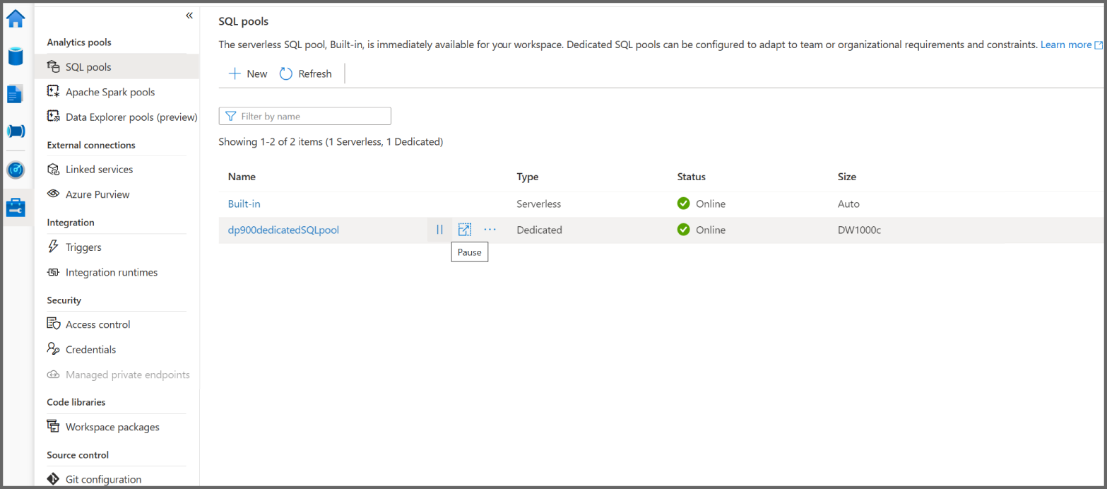
FIGURE 5.46 Pausing a dedicated SQL pool
Data Loading Methods for Dedicated SQL Pools
Traditional relational databases that use a symmetric multiprocessing (SMP) design such as SQL Server or Azure SQL Database use an ETL process for data loading. Distributed platforms that use a MPP design like Azure Synapse Analytics dedicated SQL pools can process and store large amounts of data at-scale, allowing them to leverage ELT patterns to load and transform data within the same service. This allows developers to perform data processing activities without having to rely on additional services for data transformation prior to loading.
Dedicated SQL pools support several data loading methods, including popular SQL Server methods such as the bulk copy program (bcp) utility and the SQLBulkCopy API. However, the fastest and most scalable way to load data is through the PolyBase or the COPY statement. In fact, when loading data into a dedicated SQL pool via ADF, it is recommended to set the Copy Method setting in the Sink tab to use either the Copy command or PolyBase. With PolyBase and the COPY statement, developers can access data stored in Azure Blob storage or ADLS via T-SQL commands.
Generally, both of these data loading options are best when used to load data into staging tables. Staging tables are usually defined as heap tables, or tables without any indexes. The lack of an index means that data will not be reordered as it is being written, allowing the data to be written very quickly. Staging tables can be predefined before the external table is created with a normal CREATE TABLE command or created after the external table is established with a CREATE TABLE AS SELECT (CTAS) statement. More information about the CTAS statement can be found in the section “PolyBase” later in this chapter.
Once data is loaded into the staging tables, developers can use different techniques to update production tables with the staging data. Some techniques include using the MERGE statement to insert, update, or delete data in the production table based on differences in the staging table or replacing a section of the production table with the updated staging table through a process called partition switching. More information about partition switching can be found at https://docs.microsoft.com/en-us/azure/synapse-analytics/sql-data-warehouse/sql-data-warehouse-tables-partition#partition-switching. New production tables that are based off of the staging table, but use a different distribution method and index design, can be created with a CTAS operation.
While the COPY statement offers the best performance and most flexibility for loading data, it is still important to understand how to use PolyBase to load data into a dedicated SQL pool. The following sections describe how to use PolyBase and the COPY statement to load data from Azure Storage into a dedicated SQL pool.
PolyBase
PolyBase is a data virtualization technology that enables dedicated SQL pools to query Azure Storage data while allowing the data to stay in its original location and format. PolyBase uses external tables to shape and access Azure Storage data. External tables overlay a schema on top of the data so that it can be easily queried with T-SQL commands.
Defining external tables involves specifying the data source, the format of files in Azure Storage, and the table definition. These can be defined with the following T-SQL commands:
CREATE EXTERNAL DATA SOURCECREATE EXTERNAL FILE FORMATCREATE EXTERNAL TABLE
External data sources are used to establish a connection with an Azure storage account, such as one that supports Azure Blob Storage or ADLS. The CREATE EXTERNAL DATA SOURCE command that is used to create an external data source requires the following arguments:
LOCATION—This provides the connectivity protocol and path to the data source, such asabfss://[email protected]/.CREDENTIAL—This specifies the database-scoped credential used to authenticate to the external data source. This argument is only required if the storage object does not allow anonymous access. Storage account access keys, service principals, and managed identities are the only support authentication mechanisms for Azure Storage. Developers can create a database-scoped credential with theCREATE DATABASE SCOPED CREDENTIALT-SQL command.TYPE=HADOOP—This specifies the external data source type that is being configured. It is required when the external data source is ADLS and Azure Blob Storage.
The following example creates an ADLS external data source that uses an access key to authenticate to the storage account:
/* The following creates a database master key that is used to encryptthe credential secret created in the CREATE DATABASE SCOPED CREDENTIAL step. */CREATE MASTER KEY ENCRYPTION BY PASSWORD = '<password>';/* Use the following command to create the database-scopedcredential with the storage account key. */CREATE DATABASE SCOPED CREDENTIAL dp900StorageCredentialWITHIDENTITY = 'dp900adls001' -- This is the storage account name.SECRET = '<storage_account_access_key>'CREATE EXTERNAL DATA SOURCE dp900_ADLS_Ext_SourceWITH(LOCATION = 'abfss://[email protected]/',CREDENTIAL = dp900StorageCredential,TYPE = HADOOP);
The next step in using PolyBase is to define the file format of the data stored in the external data source. External file formats created for Azure Synapse Analytics SQL pools (both dedicated and serverless SQL pools) support delimited text (such as CSV or TSV) and Parquet file formats. The CREATE EXTERNAL FILE FORMAT command accepts a required FORMAT_TYPE argument that defines the file format and several optional arguments such as how the data is compressed. Several of these optional arguments apply only to delimited text files, including:
FIELD_TERMINATOR—This specifies what character in a delimited text file marks the end of each field (column). The default field terminator is the pipe character (|).STRING_TERMINATOR—This specifies the field terminator for words or string data in a delimited text file. The default string terminator is an empty string ("").FIRST_ROW—This specifies the row number that is read first by all files.DATE_FORMAT—This specifies a specific format for date and time data in a delimited text file.
The following example creates an external file format for CSV files:
CREATE EXTERNAL FILE FORMAT dp900_CSV_File_FormatWITH(FORMAT_TYPE = DELIMITEDTEXT,FIELD_TERMINATOR = ',',STRING_TERMINATOR = '″');
Now that the external data source and external file format is defined, we can finally create the external table. The CREATE EXTERNAL TABLE command allows developers to define column names and data types for external data. It also accepts arguments for the external data source and the external file format. It also enables developers to specify the folder or the file path and filename for the data in the external data source with the optional LOCATION argument.
The CREATE EXTERNAL TABLE command also allows developers to specify reject parameters that will determine how PolyBase handles dirty records. This information is stored as metadata when the external table is created and is used when a SELECT statement is issued against the table to determine the number or percentage of rows that can be rejected before the query fails. The query will return partial results until the reject threshold is exceeded, after which the query will fail with the appropriate error message. The following arguments can be used to set the reject threshold:
REJECT_TYPE—Clarifies if theREJECT_VALUEoption is specified as a literal value or a percentage. When value is chosen, a query issued against the external table will fail when the number of rejected rows exceeds the defined value. When percentage is chosen, a query issued against the external table will fail when the percentage of rejected rows exceeds the defined threshold.REJECT_VALUE—This specifies the value or the percentage of rows that can be rejected before the query fails. When value is chosen, the argument must be an integer between 0 and 2,147,483,647. When percentage is chosen, the argument must be a decimal value between 0 and 100.REJECT_SAMPLE_VALUE—This determines the number of rows to attempt to retrieve before PolyBase recalculates the percentage of rejected rows. It is only available when percentage is chosen for the REJECT_TYPE and must be an integer between 0 and 2,147,483,647.
The following example creates an external table for the SalesLT.ProductCategory CSV file that was created in ADLS by the ADF copy activity described previously in this chapter:
CREATE EXTERNAL TABLE [dbo].[ProductCategory_External](ProductID INT,ProductSubcategoryID INT,ProductName VARCHAR(50))WITH(LOCATION = '/products/productcategory.csv',DATA_SOURCE = dp900_ADLS_Ext_Source,FILE_FORMAT = dp900_CSV_File_Format,REJECT_TYPE = VALUE,REJECT_VALUE = 0);
With the external table defined, developers can issue queries against the data without having to move the data from Azure Storage to the dedicated SQL pool. If they would like to create a copy of the data in the dedicated SQL pool, then they can do so with a CTAS statement. CTAS statements allow developers to create new tables based on the output of a SELECT statement. In a dedicated SQL pool, developers can define the distribution method and index design within the context of a CTAS statement. The following example uses a CTAS to create a dedicated SQL pool staging table based on the previously created external table:
CREATE TABLE [dbo].[ProductCategory_Staging]WITH (DISTRIBUTION = ROUND_ROBIN)AS SELECT * FROM [dbo].[ProductCategory_External]
Once the data is stored in the staging table, data engineers can perform transformations with native T-SQL queries that leverage the built-in distributed query processing capabilities of the dedicated SQL pool. Transformed data can then be moved from the staging table to a production table through a variety of methods, such as a MERGE statement, partition switching, or with an INSERT INTO SELECT statement. New production tables can also be created with a CTAS statement where the SELECT statement retrieves data from the staging table.
COPY Statement
The COPY statement is a T-SQL construct that provides the most flexibility and best performance for parallel data ingestion into an Azure Synapse Analytics dedicated SQL pool. It provides several data loading feature enhancements over PolyBase:
- Allow lower privileged users to load data without needing to grant them CONTROL permissions on the data warehouse.
- Execute a single T-SQL statement without having to create any additional objects, (i.e., external file formats, external data sources, and external tables).
- Parse and load CSV files with a more extensive list of field, string, and row delimiters.
- Access data with a finer permission model without exposing storage account access keys using a shared access signature (SAS).
- Specify a custom row terminator for CSV files.
- Use SQL Server Date formats for CSV files.
- Leverage automatic schema discovery to simplify the process of defining and mapping source data into target tables.
- Use the automatic table creation argument to automatically create the target table. This works alongside the automatic schema discovery feature.
The COPY command uses several arguments to determine how to ingest data:
FILE_TYPE—This specifies the format of the external data. Supported file formats include CSV, Parquet, and ORC.CREDENTIAL—This specifies the identity mechanism used to access the Azure storage account.MAXERRORS—This optional argument specifies the maximum number of reject rows allowed before the COPY statement is cancelled. If not specified, the default value for this argument will be 0.COMPRESSION—This optional argument specifies the data compression method for the data.FIELDQUOTE—This argument applies to CSV files and specifies the character that will be used as the quote character in the file. If not specified, the quote character (") will be used as the default value for this argument.FIELDTERMINATOR—This argument applies to CSV files and specifies the field terminator that will be used in the CSV file. If not specified, the comma character (,) will be used as the default value for this argument.ROWTERMINATOR—This argument applies to CSV files and specifies the row terminator that will be used in the CSV file. By default, the row terminator isFIRSTROW—This argument applies to CSV files and specifies the row number that is read first in all files by the COPY statement.DATEFORMAT—This argument applies to CSV files and specifies the date format of the date mapping using SQL Server date formats. Supported date formats include mdy, dmy, ymd, ydm, myd, and dym.ENCODING—This argument applies to CSV files and specifies the data encoding standard for the files. The default for this argument is UTF8, but it can be changed to UTF16 depending on the encoding standard used by the files loaded by the COPY statement.IDENTITY_INSERT—This argument is specific to values that map to an identity column in the target table. If the argument is set to off (this is the default), then the values are verified but not imported. If the argument is set to on, then the values will be imported into the identity column.AUTO_CREATE_TABLE—This argument specifies if the table could be automatically created by working alongside the automatic schema discovery feature.
A more extensive list of the arguments that can be used with the COPY statement can be found at https://docs.microsoft.com/en-us/sql/t-sql/statements/copy-into-transact-sql?view=azure-sqldw-latest&preserve-view=true#syntax.
The following example uses the COPY statement to load the SalesLT.ProductCategory CSV file from ADLS into the [dbo].[ProductCategory_Staging] dedicated SQL pool table. It assumes that the table has already been created and is empty.
COPY INTO [dbo].[ProductCategory_Staging]FROM 'https://dp900adls001.dfs.core.windows.net/dp900-adls-container/products/productcategory.csv'WITH (FILE_TYPE = 'CSV',CREDENTIAL = (IDENTITY='Shared Access Signature', SECRET = '<SAS_TOKEN>'),FIELDQUOTE = '"',FIELDTERMINATOR = ',',ROWTERMINATOR = '0X0A')
With this command, developers can quickly load data from ADLS into a dedicated SQL pool staging table and perform any computations required before moving the staging data into a production table.
Serverless SQL Pools
Azure Synapse Analytics serverless SQL pool is a serverless query service that enables users to analyze files in Azure Storage with T-SQL queries. Every workspace comes with a serverless SQL endpoint (named “Built-in”) that data analysts and developers can use to quickly begin querying data in a variety of different formats, including Parquet, CSV, and JSON. Additionally, serverless SQL pools can be used to query Azure Cosmos DB with Azure Synapse Link and Spark tables that are created with Azure Synapse Analytics Apache Spark pools.
Typical use cases for serverless SQL pools are as follows:
- Basic discovery and exploratory analysis with SQL queries. Analysts can use the OPENROWSET function in the FROM clause of a SELECT statement to access data in several different formats (Parquet, CSV, JSON, and Delta) from Azure Storage without having to persist the connection information in a separate object.
- Creating a logical data warehouse to provide a relational schema on top of raw data in Azure Storage without moving or creating a second copy of the data. Logical data warehouses in serverless SQL pools are complete with familiar relational database constructs such as databases, tables, and views.
- Streamlining data transformation activities with T-SQL and loading the transformed data back into Azure Storage or into a persistent relational data store (such as a dedicated SQL pool or Azure SQL Database). Transformed data can also be served directly to BI tools like Power BI.
Logical data warehouses that are built with serverless SQL pools use similar data virtualization techniques as those that are used with dedicated SQL pools, including external data sources to connect to storage accounts, external file formats that define the format of the data in Azure Storage, and external tables that define a schema for your external data sources. The primary difference is that external data sources are native to synapse SQL pools and do not require (or support) the TYPE=HADOOP argument. More information about using these constructs to create a logical data warehouse with a serverless SQL pool can be found at https://docs.microsoft.com/en-us/azure/synapse-analytics/sql/tutorial-logical-data-warehouse.
Just like dedicated SQL pools, serverless SQL pools support several management tasks and tools that are common to the Microsoft suite of SQL offerings. Developers can choose to run ad hoc queries against a serverless SQL pool endpoint from Synapse Studio or via common client tools like Azure Data Studio and SQL Server Management Studio (SSMS). Furthermore, database administrators can manage authentication and authorization with SQL authentication and Azure AD.
While serverless and dedicated SQL pools both leverage distributed processing architectures that are designed to manage large datasets, when to use one or the other depends on use case requirements and the acceptable cost-to-performance threshold. Serverless SQL pools use a pay-per-query cost model, only charging users for the amount of data processed by each query. This cost model provides a cheap alternative to dedicated SQL pools for quickly analyzing data with ad hoc queries. However, because storage is not local to the serverless SQL pool and compute is automatically scaled, queries tend to run slower (a factor of seconds or minutes) than queries executed against a dedicated SQL pool. For this reason, dedicated SQL pools are a better option for workloads that require optimized and consistent performance requirements.
Exploratory Analysis with Serverless SQL Pools
Synapse Studio makes it easy to start analyzing data with the serverless SQL pool by creating a new SQL script. To do this, click on the Develop button on the left-side toolbar and click on the + icon. Select SQL script to open a new SQL script window. Within the script window, you can write SQL scripts that use the serverless SQL pool or one of the dedicated SQL pools associated with the workspace. The properties pane on the right side of the script window allows you to rename the script and add a description that explains the functionality of the script. You can also save scripts in Synapse Studio or to an associated Git repository by clicking Publish All at the top of the script window. Figure 5.47 illustrates the layout of the SQL script window.

FIGURE 5.47 Synapse Studio SQL script window
The ribbon at the top of the SQL script window includes several options for running a script, viewing a query's execution plan (exclusive to dedicated SQL pools), connecting to a SQL pool, and setting the database context. To execute queries with the serverless SQL pool endpoint, make sure the “Built-in” SQL pool is chosen in the Connect To drop-down menu (see Figure 5.48).

FIGURE 5.48 Choosing the Built-in SQL pool
Before going over how to run queries in Synapse Studio, let's briefly discuss the basic structure of a serverless SQL pool query. Serverless SQL pool queries that perform exploratory analysis rely heavily on the OPENROWSET function to read data from external storage devices. For example, the following query uses the OPENROWSET function to retrieve the first 100 entries of the publicly available New York City yellow taxicab dataset.
SELECTTOP100 * FROMOPENROWSET(BULK 'https://azureopendatastorage.blob.core.windows.net/nyctlc/yellow/puYear=*/puMonth=*/*.parquet',FORMAT='PARQUET') AS [nyc]
The BULK parameter specifies the location of the data while FORMAT specifies the file format of the data being read. The URL location used by the query also uses wildcards (*) to read all of the Parquet files in all of the year and month folders.
This query also uses the column metadata in the Parquet files to infer the column names and data types of the result set. Queries can also automatically infer the column names of data from CSV files if there is a header row. However, there are times where you will want to explicitly define a schema to have more control of the data. Explicitly defining a schema also allows you to specify what columns you want to read from the files. You can define a schema for your data by adding a WITH clause with the column names and data types at the close of the OPENROWSET command. The following example uses the WITH clause to explicitly return three columns from the New York City yellow taxicab dataset.
SELECTTOP100 * FROMOPENROWSET(BULK 'https://azureopendatastorage.blob.core.windows.net/nyctlc/yellow/puYear=*/puMonth=*/*.parquet',FORMAT='PARQUET') WITH (tpepPickupDateTime DATETIME2,passengerCount INT,tripDistance FLOAT) AS [nyc]
Passing the entire storage URL into the BULK parameter is a quick and easy way to read the content of the files with basic authentication methods such as Azure AD authentication for Azure AD logins or from files that are publicly available. However, this option provides limited authentication options and can become tedious as it forces developers to add the storage URL to the BULK parameter when they query the storage account. A more repeatable and secure option is to persist the location as an external data source and the access credential as an external scoped credential in a serverless SQL pool logical database.
The following example creates a new logical database and an external data source that references the location of the New York City yellow taxicab dataset. You can then pass the external data source name to the optional DATA_SOURCE parameter in the OPENROWSET command. This allows you to alter the argument passed to the BULK parameter to only the folder path that needs to be queried.
CREATE DATABASE dp900_serverlessdb;USEdp900_serverlessdbGO;CREATEEXTERNAL DATA SOURCE nyc_yellowcabWITH(location = 'https://azureopendatastorage.blob.core.windows.net/nyctlc/yellow/');SELECT TOP 100 * FROMOPENROWSET(BULK 'puYear=*/puMonth=*/*.parquet',DATA_SOURCE='nyc_yellowcab',FORMAT='PARQUET') WITH (tpepPickupDateTime DATETIME2,passengerCount INT,tripDistance FLOAT) AS [nyc]
This script can be executed in the Synapse Studio SQL script window by clicking the Run button at the top of the window. Figure 5.49 shows the SQL script window and the results from the executed script.

FIGURE 5.49 Executing Serverless SQL Pool Queries in Synapse Studio
More information about how to use OPENROWSET to query external data with a serverless SQL pool can be found at https://docs.microsoft.com/en-us/azure/synapse-analytics/sql/develop-openrowset.
Summary
This chapter started by discussing different types of data workflows. Transactional systems, also known as online transaction processing (OLTP) systems, capture business transactions such as sales in a point-of-sale system. They are optimized to handle write-heavy workloads, often handling millions of transactions a day. Analytical systems differ from transactional systems in that they are optimized for read-heavy operations. Data is gathered from several source systems and consolidated in one or a few data stores that users can use for reports, ad hoc analysis, and data science projects.
Analytical systems can process data in batches or as a continuous stream of data. Batch processing involves processing large amounts of data at predetermined periods of time or after a specified event. Stream processing ingests and transforms data in real time as it is generated. Modern data architectures like the Lambda architecture make it easy to use both batch and stream processing in the same solution.
There are several services offered through Azure that data engineers can use when building a modern data warehouse solution. Azure HDInsight is a PaaS resource that can be used to build data processing pipelines with several popular open-source frameworks such as Apache Hadoop, Apache Spark, Apache Kafka, Apache HBase, Apache Interactive Query, and Apache Storm. Azure Databricks is another PaaS resource that provides a unified platform for data engineers building data processing pipelines with Databricks Spark. Databricks Spark is a highly optimized version of Apache Spark, making it the most ideal service for most Spark applications.
Azure HDInsight, Azure Databricks, and several other data movement and data transformation activities can be orchestrated with Azure Data Factory (ADF). ADF enables data engineers to build data engineering pipelines with the Azure Data Factory Studio, a drag-and-drop, low-code/no-code development environment. Developers can author data movement and data transformation activities to run in parallel or chain them together so that they run sequentially. Because ADF is a PaaS offering, compute infrastructure is abstracted from the user in the form of an integration runtime. However, users can choose to use their own compute infrastructure by installing a self-hosted integration runtime on a virtual machine. This allows users to leverage data sources that are located in on-premises and private networks.
Organizations that want to use a single platform to achieve end-to-end analytics can do so with Azure Synapse Analytics. With Azure Synapse Analytics, users can use the Synapse Studio to manage all aspects of the data processing life cycle. Developers can author low-code/no-code data integration pipelines to move and transform data, leverage the serverless SQL pool to explore operational and object data stores with T-SQL without moving the data, build scale-out data engineering solutions with Apache Spark pools, and store report-ready data in relational tables that are optimized to serve analytical queries with a dedicated SQL pool.
Exam Essentials
- Describe the difference between transactional and analytical workloads. Transactional systems are used to capture the business transactions that support the day-to-day operations of a business, while analytical systems turn transactional data and other data sources into information that is used to make decisions. Remember that transactional data is highly normalized to support write operations, and analytical data is denormalized to support read operations. Depending on the use case, analytical workloads can store data in a relational data warehouse such as Azure Synapse Analytics dedicated SQL pool or as files in an enterprise data lake such as ADLS.
- Describe batch and stream processing. Data engineers can build data processing pipelines with one or a combination of two techniques: batch processing and stream processing. For the DP-900 exam, remember that batch processing workflows process data in batches during a predetermined period of time or after a specific event. Stream processing workflows ingest and transform continuous streams of data in real time. Know the technologies that were listed for each component of the two processing types. Also remember that modern, cloud-based architectures make it easy to implement batch processing and stream processing workflows in the same solution.
- Describe data warehouse features. Remember that data warehouses store data that is optimized for analytical queries and are commonly used as the single source of truth for data that is important to a business department's decision making. Data models follow the star schema design pattern, where business entities and descriptors related to them are stored in dimension tables and measured events related to business entities are stored in fact tables.
- Describe Azure HDInsight. Azure HDInsight is a managed, open-source analytics service in Azure that can be used to deploy distributed clusters for Apache Hadoop, Apache Spark, Apache Interactive Query/LLAP, Apache Storm, Apache Kafka, and Apache HBase. Remember that unlike Azure Databricks and Azure Synapse Analytics Apache Spark pools, Azure HDInsight clusters cannot be paused. You will need to destroy the cluster and build a new one with an automation script to manage Azure HDInsight costs. For this and other management reasons, it is recommended that you use other Azure services like Azure Databricks, Azure Synapse Analytics, and the Azure Event Hubs Kafka endpoint for distributed analytics.
- Describe Azure Databricks. Azure Databricks is a unified analytics platform that supports optimized Spark clusters for batch and stream processing. The platform is a PaaS resource that provides a native notebook environment that developers can use to build Spark workflows with SQL, Python, Java, or R. Remember that Databricks clusters use Azure VMs for compute nodes and that processing is measured as Databricks Units (DBUs). Databricks clusters can be configured as dedicated compute for single user, prescheduled processing jobs (Single Node or Standard), or to run concurrent workloads for multiple users performing interactive analysis (High Concurrency). Remember that you can establish a connection with an Azure storage account by creating a mount point or by using a service principal to connect via a direct path. ADLS accounts can also be accessed directly with Azure AD credential passthrough.
- Describe Azure Data Factory. Azure Data Factory (ADF) is a managed cloud service that can be used to build complex ETL, ELT, and data integration projects. ADF instances provide data engineers with a platform to author no-code data movement and data transformation activities and run them sequentially or in parallel with pipelines. ADF pipelines can be executed manually or automatically via a schedule or an event-based trigger. Users can define connections to over 90 data sources and compute resources as linked services. Linked services that are created for data sources can be used to represent specific data structures within data stores, such as a relational database table or a set of files. Remember that integration runtimes are the compute infrastructure that power pipeline activities. Integration runtimes come in three types: one for Azure resources that are accessible via a public endpoint, a self-hosted integration runtime for on-premises resources or Azure resources that are only accessible through a private network, and an SSIS specific integration runtime that allows users to run legacy SSIS packages in an ADF pipeline.
- Describe Azure Synapse Analytics. Azure Synapse Analytics is an enterprise analytics system that unifies multiple services that serve analytical workloads in a single environment. Within Synapse Studio, data engineers can use Synapse pipelines to automate data movement and processing activities, a dedicated SQL pool as an analytical data store to manage data that will need to quickly serve reports and analytical applications, a serverless SQL pool to interactively query data in Azure Storage, an Apache Spark pool to perform data engineering activities with Spark, and a Data Explorer pool to analyze telemetry data in near real time. Analysts can also link a Power BI workspace to an Azure Synapse Analytics workspace to build reports in the same environment that they manage data and write queries.
Review Questions
- Is the italicized portion of the following statement true, or does it need to be replaced with one of the other fragments that appear below? Relational databases that serve transactional workloads often use a star schema as their data model strategy. This modeling pattern is optimal for write-heavy operations.
- 1NF
- 3NF
- 2NF
- No change needed
- Which of the following data storage options are appropriate for data scientists and analysts to use when analyzing business data?
- Data warehouses
- OLAP models
- Enterprise data lakes
- All of the above
- What open-source technology provides ACID properties on data stored in ADLS?
- Delta Lake
- Parquet
- Apache Spark
- Hadoop
- Which of the following services is not used in a batch processing workflow?
- Azure Databricks
- Azure Stream Analytics
- Azure Synapse Analytics
- Azure Data Factory
- You are designing a data warehouse that will serve as the single source of truth for a venue management company. The data warehouse's data model will use a star schema so that it is optimized for reporting tools and analytical queries. Using this design pattern, what type of tables will store concession and retail sales metrics?
- Dimension tables
- Materialized views
- Fact tables
- Composite tables
- You are designing a stream processing pipeline for an IoT workflow. The solution will use Apache Spark structured streaming to process the data, but it requires a highly scalable service to act as the real-time message ingestion engine. Which of the following Azure HDInsight cluster types is a viable option to ingest large volumes of streaming data?
- Apache Hadoop
- Apache Spark
- Apache Kafka
- Apache Storm
- Which of the following statements about Azure Databricks is false?
- Azure Databricks cannot read data from a real-time ingestion engine like Azure Event Hubs or Apache Kafka.
- Administrators can leverage their existing Azure Active Directory infrastructure to manage user access control for Databricks-specific objects such as notebooks, clusters, and jobs.
- Azure Databricks can read and write data from Azure data stores such as Azure Blob Storage, ADLS, Azure SQL Database, and Azure Synapse Analytics dedicated SQL pools.
- When creating a Spark cluster in Azure Databricks, users can set a time period that Azure Databricks will use to automatically terminate the cluster when idle.
- Which of the following components is not used when calculating the cost of an Azure Databricks cluster?
- Azure VM price
- Price of DBUs consumed
- Azure Databricks workspace price
- None of the above
- You are deploying a new Azure Databricks workspace that will be used by data engineers and data scientists at your company. Clusters deployed to the workspace will need to be able to connect to Azure services that are assigned private endpoints. You are also required to configure Azure Databricks so that cluster nodes do not have public IP addresses. Which of the following options is the recommended solution for meeting the listed requirements?
- Enable VNet injection on the workspace so that all cluster nodes run on one of your VNets. This will allow you to easily connect clusters to services using private endpoints. VNet injection uses all private IP addresses by default.
- Enable VNet injection on the workspace so that all cluster nodes run on one of your VNets. This will allow you to easily connect clusters to services using private endpoints. Enable secure cluster connectivity to change the public subnet to private.
- Enable VNet injection on the workspace so that all cluster nodes run on one of your VNets. This will allow you to easily connect clusters to services using private endpoints. Enable private link to change the public subnet to private.
- Use VNet peering to peer the Databricks-managed VNet with the VNet that hosts the private endpoints you are connecting to. VVet injection uses all private IP addresses by default. Enable secure cluster connectivity to ensure that only private IP addresses are used.
- Which of the following Git providers are supported by Azure Databricks?
- Bitbucket
- GitHub
- Azure DevOps
- All of the above
- You are configuring an Azure Databricks cluster that will be used by several analysts and data scientists. Because users will be running interactive workloads sporadically, the cluster must be able to support concurrent requests. Which cluster mode should you define for this cluster?
- Standard
- High Concurrency
- Single User
- Interactive
- Which of the following is not a component that can be manually created after an Azure Synapse Analytics workspace is deployed?
- Serverless SQL pool
- Dedicated SQL pool
- Data Explorer pool
- Apache Spark pool
- You are designing a solution that will analyze operational data that is stored in an Azure Cosmos DB Core (SQL) API database. The solution must be near real time, but it must also minimize the impact on the performance of the operational data store. Which of the following options is the most appropriate for this scenario?
- Enable Azure Synapse Link to synchronize your transactional data from Azure Cosmos DB to a column-oriented analytical data store and use an Azure Synapse Analytics serverless SQL pool to analyze the data.
- Create an Azure Data Factory copy activity to copy the data from Azure Cosmos DB to an Azure Synapse Analytics dedicated SQL pool.
- Create an Azure Data Factory copy activity to copy the data from Azure Cosmos DB to an Azure Synapse Analytics serverless SQL pool.
- Enable Azure Synapse Link to synchronize your transactional data from Azure Cosmos DB to a column-oriented analytical data store and use an Azure Synapse Analytics data explorer pool to analyze the data.
- How many additional Azure Synapse Analytics serverless SQL pools can be added to a single workspace?
- 1
- 10
- 0
- 5
- You are the administrator for an Azure Synapse Analytics dedicated SQL pool. Table distribution and index design are optimized to meet the workload needs of the queries that are frequently executed against the database. You have recently been asked to improve the performance of a query that is run regularly. When enabled, which of the following features will immediately improve the query's performance by caching the results for later use?
- Result set caching
- Query store
- Extended events
- Clustered columnstore index
- Which of the following is a common use case for an Azure Synapse Analytics serverless SQL pool?
- Performing exploratory analysis of Azure Storage data with T-SQL queries
- Creating a logical data warehouse that maintains an up-to-date view of data by providing a relational schema on top of raw data stored in Azure Storage without moving data
- Transforming ADLS data with T-SQL and serving the transformed data to Power BI or a persistent data store like Azure SQL Database
- All of the above
- What T-SQL function allows you to read the content of files stored in Azure Storage with a serverless SQL pool?
- OPENQUERY
- OPENROWSET
- OPENDATASOURCE
- OPENEXTERNALDATA
- Is the italicized portion of the following statement true, or does it need to be replaced with one of the other fragments that appear below? A Serverless SQL pool is an analytical data store that uses a scale-out architecture to distribute data processing across multiple nodes. It is optimized to serve large amounts of historical data very quickly to data analysts and BI applications and is typically used as the single source of truth for business insights.
- Dedicated SQL pool
- Data Explorer pool
- Apache Spark pool
- No change needed
- What type of Azure Data Factory activity is used to manage the flow of a pipeline?
- Data movement activity
- Control activity
- Data transformation activity
- Compute activity
- Which of the following options can you use with an ADF copy activity to define what data is copied from an Azure SQL Database table?
- The entire table
- The result set from a query
- The result set from a stored procedure
- All of the above
- You are the lead data engineer for a company that is modernizing its existing data platform to Azure. One part of the modernization effort is to lift and shift existing SSIS packages to Azure and use PaaS infrastructure to run the SSIS packages. Which of the following is a valid approach in Azure while minimizing infrastructure overhead?
- Deploy the existing packages to an SSISDB database hosted on an Azure SQL Database and execute them with the SQL Server Agent.
- First, deploy the existing packages to an SSISDB database hosted on Azure SQL Database. Next, create an Azure-SSIS integration runtime in an Azure Data Factory instance and use the Execute SSIS Package activity with the integration runtime to run the SSIS packages.
- Deploy the existing packages to an SSISDB database hosted on a SQL Server Azure VM and execute them with the SQL Server Agent.
- First, deploy the existing packages to an SSISDB database hosted on Azure SQL Database. Next, create a self-hosted integration runtime in an Azure Data Factory instance and use the Execute SSIS Package activity with the integration runtime to run the SSIS packages.
- ADF pipelines can be deployed manually, at a scheduled time, and after which one of the following event types?
- After a blob is uploaded to Azure Blob storage
- After a new row of data is inserted into a SQL Server database table
- After a new item is added to an Azure Cosmos DB database container
- All of the above
- You are designing a data ingestion strategy that uses PolyBase to load CSV data from ADLS into an Azure Synapse Analytics dedicated SQL pool. When defining the external file format, what argument and terminator character should you use to indicate the end of each field in the files?
FIELD_TERMINATOR = '|'STRING_TERMINATOR = '|'STRING_TERMINATOR = ','FIELD_TERMINATOR = ','
- You are building a data ingestion solution that will perform a one-time load of ORC data from ADLS into an Azure Synapse Analytics dedicated SQL pool staging table. Which of the following options provides the best performance for this use case?
- Build the solution using PolyBase constructs, creating an external table that provides a schema for the ORC data. Once the external table is created, use a CTAS statement to create the staging table based on the PolyBase external table.
- Copy the data into the staging table using the bulk copy program (bcp) utility.
- Copy the data into the staging table using a COPY statement.
- Copy the data into the staging table using AzCopy.