
Chapter 1
Core Data Concepts
This chapter will focus on the first objective for the Microsoft Azure DP-900 exam certification: describe core data concepts. We will discuss the different types of data and how they are stored, data processing techniques, and categories of data analytics. Understanding the concepts covered in this chapter is critical to designing the most appropriate modern data solution in Azure for any business problem.
Describe Types of Core Data Workloads
The volume of data that the world has generated has exploded in recent years. Zettabytes worth of data is created every year, the variety of which is seemingly endless. Competing in a rapidly changing world requires companies to utilize massive amounts of data that they have only recently been exposed to. What's more is that with the use of edge devices that allow Internet of Things (IoT) data to seamlessly move between the cloud and local devices, companies can make valuable data-driven decisions in real time.
It is imperative that organizations leverage data when making critical business decisions. But how do they turn raw data into usable information? How do they decide what is valuable and what is noise? With the power of cloud computing and storage costs growing cheaper and cheaper every year, it's easy for companies to store all the data at their disposal and build creative solutions that combine a multitude of different design patterns. For example, modern data storage and computing techniques allow sports franchises to create more sophisticated training programs by combining traditional statistical information with real-time data captured from sensors that measure features such as speed and agility. E-commerce companies leverage click-stream data to track a user's activity while on their website, allowing them to build custom experiences for customers to reduce customer churn.
The exponential growth in data and the number of sources organizations can leverage to make decisions have put an increased focus on making the right solution design decisions. Deciding on the most optimal data store for the different types of data involved and the most optimal analytical pattern for processing data can make or break a project before it ever gets started. Ultimately, there are four key questions that need to be answered when making design decisions for a data-driven solution:
- What value will the data powering the solution provide?
- How large is the volume of data involved?
- What is the variety of the data included in the solution?
- What is the velocity of the data that will be ingested in the target platform?
Data Value
The first question that needs to be answered when designing a data-driven solution is, what value will be gained by processing, storing, and analyzing potential data sources? What answers are the business trying to solve? While it is true that having more data can provide new and more fine-grained insights, it can sometimes come at a cost. Organizations must give considerable thought to what data is valuable and what data is not, all the while trying to minimize the amount of time spent in the decision-making process.
Designing a data-driven solution requires everyone involved to focus on deriving value from every process in the solution. This means that data architects must know the business goal of the solution from the beginning. Is this going to be a transactional database that provides the backend for a business's e-commerce site? Will it be a data warehouse aggregating data from multiple source systems to provide a holistic view of a business's performance? Or will the data store need to be able to ingest bursts of IoT data for real-time analytics? To answer these questions, we first need to understand the different types of data stores and the scenarios for which each one is best suited.
Relational Databases
Relational databases organize data into tables that can be linked based on data common to each other. The relationship between tables allows users to easily query multiple tables in the same query by joining columns from multiple tables together. Database tables store data as rows and are organized into a set number of columns. Columns are defined by specific data types such as integer or string so that only specific types of data from new or modified rows of data is accepted. For example, if you have a database table with a name column that only accepts string values, then trying to insert a number into that column will fail. Relational databases allow designers to go a step forward and design constraints on columns so that data must meet predefined criteria. This predefined structure that data in relational databases must adhere to is called a schema and is fundamental to how users query relational data.
Users querying a relational database use a version of the Structured Query Language (SQL) to issue queries to the database. Depending on the vendor, most relational database management systems (RDBMSs) have their own variation of SQL that are based on the ANSI standardized version of SQL. For example, the Microsoft suite of RDBMSs (e.g., SQL Server, Azure SQL Database, Azure SQL Managed Instance) can be interacted with using Transact SQL (T-SQL). T-SQL provides four flavors of commands for query development:
- Data Manipulation Language (DML) commands are used to manipulate data in database tables. DML commands include SELECT, INSERT, UPDATE, and DELETE.
- Data Definition Language (DDL) commands are used to define RDBMS objects such as databases, tables, views, stored procedures, and triggers. DDL commands include CREATE, ALTER, and DROP.
- Data Control Language (DCL) commands are used to manage permissions and access control for users in a database. DCL commands include GRANT, REVOKE, and DENY.
- Transaction Control Language (TCL) commands are used to explicitly manage and control transaction execution to ensure that a specific transaction is successfully done without violating database integrity. TCL commands include BEGIN TRANSACTION, COMMIT TRANSACTION, and ROLLBACK TRANSACTION.
Relational database design considerations largely depend on what the database will be supporting. A database that's supporting a business's e-commerce site and needs to log every transaction made by a customer has vastly different requirements than a database that supports a report application. While there are many different design patterns for data-driven solutions, most of them fall into one of two broad categories: transactional processing systems or analytical systems.
Transactional Processing Systems
Transactional processing systems, also known as online transaction processing (OLTP) systems, are used to capture the business transactions that support the day-to-day operations of an organization. Transactions can include retail purchases logged to point-of-sale (PoS) systems as purchases are made, orders purchased through e-commerce platforms, or even ticket scans at a sport or concert venue. Transactions do not only consist of newly inserted data, but also include deletes and updates of data. While each transaction is a small and unique measurement of work, OLTP systems need to be able to handle millions of transactions a day. This requires OLTP systems to be designed in a way that optimizes how fast transactions are applied to them. To support this requirement, OLTP data stored in relational databases is split into small chunks and stored in separate database tables. Splitting data into multiple tables allows the system to only update the tables that need to be updated, all the while maintaining relationships to data in tables that are associated but not updated with that transaction. This is commonly referred to as normalizing data.
Transactional databases must adhere to ACID properties (atomicity, consistency, isolation, durability) to ensure that each transaction is reliable. These properties can be defined as follows:
- Atomicity guarantees that each transaction is treated as a single unit of work that either succeeds completely or fails completely. If any part of an insert, delete, or update operation in a transaction fails, the entire transaction fails and the database is left unchanged.
- Consistency ensures that data affected by a transaction is valid according to all predefined rules. Inserting or altering data will only be successful if it maintains the appropriate predefined data types and constraints of the affected columns.
- Isolation ensures that concurrent transactions do not affect one another.
- Durability guarantees that once a transaction has been committed, it will remain committed even if there is a system failure.
Adhering to ACID properties is critical for OLTP systems that support many concurrent users reading and writing from them at the same time. They need to be able to process transactions in isolation, all the while ensuring that users querying data can retrieve a consistent view of data even as it is being altered. Many RDBMSs implement relational consistency and isolation by applying locks to data when it is updated. A lock prevents other processes from reading data until the lock is released, and it is only released when the transaction is committed or is rolled back. Extensive locks caused by long-running queries can lead to poor query performance. To mitigate the issues caused by table locks, SQL Server and Azure SQL Database give database administrators (DBAs) the ability to specify the level of isolation to which one transaction must be isolated from data modifications made by other transactions. Isolation levels determine the acceptance rate for queries returning data that has not been committed by an insert, update, or delete for faster return times. More on isolation levels can be found in Chapter 2, “Relational Databases in Azure.”
Analytical Systems
Analytical systems are designed to support business users who need to make informed business decisions from large amounts of data. For example, decisions made from analytical systems can drive the placement of an item in a retail store or an e-commerce site based on an item's seasonal popularity. Most analytical systems ingest data from multiple sources, such as OLTP systems, and perform transformations that leverage business rules that cleanse and aggregate data so that it is useful for decision making. Decision makers usually don't need all the details of a specific transaction, so data architects will design analytical systems that use data from OLTP systems to only include relevant information. Analytical systems are also denormalized so that users querying them are not burdened by having to develop complex queries that join multiple tables together. Analytical systems such as data warehouses are updated by either processing batches of data at the same time or aggregating data in real time from sources that can stream data. These different data-processing techniques are discussed further in the section “Data Velocity” later in this chapter.
The two types of analytical systems are data warehouses and online analytical processing (OLAP) systems. Data warehouses serve as the single source of truth for different functional areas within a business. Good data warehouses consolidate multiple disparate data sources and are optimized for reading data, making them perfect data sources for reporting applications. Data warehouses are typically relational data stores such as Azure Synapse Analytics dedicated SQL pool or Azure SQL Database. OLAP models are typically business intelligence (BI) models that apply business logic and pre-aggregations to data warehouse data to create a layer of abstraction between the data warehouse and a reporting platform. Azure Analysis Services and Power BI tabular models are examples of OLAP technologies that can create these types of data models.
Typical data warehouses and OLAP tabular models will store data using a star schema. Star schemas make data easy to report against because of the way data is denormalized. Measurements and metrics are consolidated in fact tables. They are connected to tables that contain descriptive attributes for each measurement, also known as dimension tables. For example, an Internet sales fact table can be associated to multiple dimension tables, that include a date dimension that provides granular information on the date a purchase was made, a customer dimension that includes specific information about the customer that made the purchase, and a product dimension that describes the different attributes of the product that was sold. The inherent simplicity in a star schema's design allows analysts to easily create aggregations on fact tables while joining the necessary dimension tables to answer different business questions about the data.
Nonrelational Data Stores
There is a wide variety of data that doesn't fit in a relational model. Nonrelational data, also known as NoSQL (Not Only SQL), refers to data that doesn't fit into a relational model. Some solutions require more flexible data models than that of a relational database and can afford to trade ACID compliancy for speed and horizontal scale. NoSQL databases can handle volatile data that is written and read quickly better than relational databases because they don't force the data to conform to a specific structure.
Binary objects such as images, videos, and PDFs are also considered nonrelational data. While relational databases such as SQL Server can store files such as the PDF copy of this book using features such as FILESTREAM, it is not the most optimal solution for file storage. Object stores are optimized for binary file storage and can be easily accessed to serve these files to applications. They can also be used to create highly scalable data lake ecosystems for big data processing solutions.
NoSQL Databases
NoSQL databases do not impose a schema on data they store, allowing data to maintain its natural format as it is ingested. In fact, one of the primary benefits is that users who are designing a NoSQL database solution do not need to define the schema ahead of time. This flexibility makes NoSQL databases the ideal choice for solutions that require millisecond response times and need to be able to scale rapidly. Scenarios where NoSQL databases are potentially better options than relational databases include ingesting and analyzing bursts of data from IoT sensors, storing product catalog data for an e-commerce site's web search functionality, and storing user-generated content for web, mobile, and social media applications.
Instead of storing data as rows in a table as in a relational database, data is stored as entities in collections or containers. Unlike rows in a table, entities in the same collection can have a different set of fields. This flexibility allows for several different implementations of NoSQL databases depending on the solution requirements. Generally, these implementations fall into the following four categories:
- Key-value stores are the simplest types of NoSQL database for inserting and querying data (see Figure 1.1). Each piece of data contains a key and a value. The key serves as a unique identifier for the piece of data, and the value contains the data. Values can be scalar values or complex structures such as a JSON array. When applications are querying data from key-value stores, they issue queries that specify the keys to retrieve the values. Figure 1.1 is an example of a phone directory that stores one or more phone numbers per person in a key-value store. Examples of key-value stores include Python dictionary objects, Azure Table storage, and the Azure Cosmos DB Table API.

FIGURE 1.1 Key-value store
- Document databases are the most common types of NoSQL databases (see Figure 1.2). Pieces of data are defined as documents and are typically stored in JSON, XML, YAML, or BSON format. Each document includes a document key that serves as a unique identifier for management and query lookups. Unlike a key-value store that can only retrieve data by doing a search on the key, applications querying a document database can perform lookups on a document's key and/or one or more of its fields to retrieve specific sets of data. This feature makes document databases a better option for applications that need to be more selective. Figure 1.2 illustrates an example of customer orders stored as documents in a document database. Examples of document databases include MongoDB and the Azure Cosmos DB Core (SQL) API.

FIGURE 1.2 Document database
- Columnar databases appear like relational databases conceptually (see Figure 1.3). They organize data into rows and columns but denormalize data so that it is divided into multiple column families. Each column family holds a set of columns that are logically related. Figure 1.3 is an example of a bicycle company's product information stored in a columnar format. An example of a columnar database is the Azure Cosmos DB Cassandra API.

FIGURE 1.3 Columnar database
- Graph databases store data as entities and focus on the relationship that these entities have with each other (see Figure 1.4). Entities are defined as nodes, while the relationships between them are defined as edges. Applications querying a graph database do so by traversing the network of nodes and edges, analyzing the relationships between entities. While relational databases can accomplish similar goals, large graph databases can perform very traverse relationships very quickly bypassing the need to perform multiple join operations on many tables. Figure 1.4 illustrates an example of a graph database that stores an organization's personnel chart. The entities represent different job titles and departments, while the edges represent how each entity is related. Examples of graph databases include Neo4j and the Azure Cosmos DB Gremlin API.
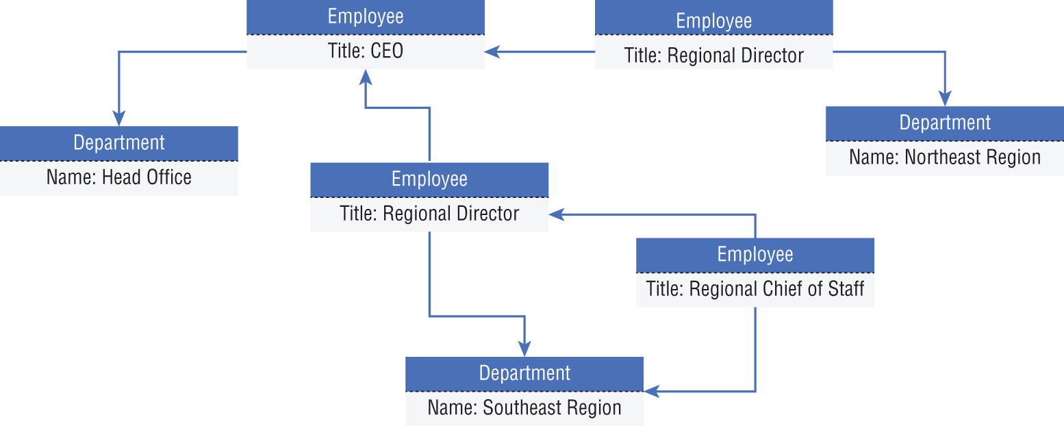
FIGURE 1.4 Graph database
Object Storage
Object data stores such as Azure storage accounts store huge volumes of data in text and binary format. You can think of a storage account as being like a shared folder on an organization's local network. Unlike local file shares, storage accounts are highly scalable and allow organizations the freedom of being able to add whatever data they want without needing to worry about adding hardware. Azure-based solutions that rely on data stored in files leverage Azure storage accounts in some form, as in the following scenarios:
- Storing images or videos that are analyzed by deep learning models or that are served to a website
- Storing files such as JSON, Avro, Parquet, CSV, or TSV that are used for distributed processing in big data solutions
- Storing data for backup and restore, disaster recovery, and archiving
- Storing telemetry information as log files that can be used for near real-time analysis
Storage accounts can service a wide variety of object store use cases. Depending on the scenario, you may decide to use one of the following storage account services to store binary objects:
- Azure Blob Storage is the most common service for object storage in Azure. Solutions that require analysis, from images or videos, backup management, or files used for distributed processing solutions, can be stored in Blob Storage. It can store exabytes worth of data and offers different access tiers to store data in the most cost-effective manner.
- Azure Data Lake Storage Gen2, also known as ADLS, is a set of capabilities that are built on top of Blob Storage but specifically for distributed analytics solutions. The key feature of ADLS that allows for quick and efficient data access is its hierarchical namespace. Hierarchical namespaces organize files into a hierarchy of directories that enable you to store data that is raw, cleansed, and aggregated without having to sacrifice one copy for the next.
- Azure Files is a fully managed file share solution in Azure. File shares are accessible via the Server Message Block (SMB) protocol or the Network File System (NFS) protocol. They can be mounted concurrently by cloud or on-premises systems.
Data Volume
Data volume refers to the amount of data that needs to be analyzed and processed. Access to larger datasets can provide just as many headaches as it does clarity. Large datasets that are stored in databases that use bad design practices or queried by poorly written queries can cause applications to perform so badly that they come to a screeching halt. Traditional relational databases such as SQL Server or Azure SQL Database can be used for large data warehouses if they are leveraging a well-thought-out data model design with appropriate indexes and partitions, and applications are reading data with well-written queries. However, there is a limit to the amount of data that traditional database technologies and processing patterns can handle.
It is critical that the right data storage technologies and processing patterns are chosen in the design phase, especially if the datasets are going to be large in volume. Even the most properly tuned relational databases will begin to perform poorly after a certain size threshold. Symmetric multiprocessing, or SMP, systems such as SQL Server and Azure SQL Database are characterized by a single instance of an RDBMS that shares all the resources (CPU, memory, and disk). SMP systems can scale up to serve gigabytes (GB) and terabytes (TB) worth of data but hit a wall when the resource limits are hit. Massively parallel processing, or MPP, systems such as Azure Synapse Analytics dedicated SQL pool are designed to process large datasets. MPP systems are designed to be distributed parallel processing solutions, meaning they are not only able to scale up by adding more compute resources but can also scale out by adding more nodes to the system.
You can think of data processing differences between SMP and MPP systems as how a grocery store goes about restocking its shelves. One employee of a store can efficiently restock shelves in a single aisle in a relatively short amount of time. However, restocking every aisle in a large store that has many aisles can take hours or even days if there is only one employee available for the task. In most cases, floor managers at a store will assign aisles to different employees. This drastically reduces the amount of time it takes to restock an entire store since there are many employees restocking shelves in parallel. This is how MPP systems such as Azure Synapse Analytics, Azure HDInsight, and Azure Databricks operate. The underlying architecture includes a driver/control node that divides large processing tasks into multiple operations and assigns them to different worker/compute node. Data is stored in a distributed file system that is split into chunks to be processed by the different worker nodes.
The ability to separate compute and storage allows MPP systems to scale very quickly. Adding nodes to an Azure Synapse Analytics dedicated SQL pool or an Azure Databricks cluster can happen without having to repartition data. Data is instead persisted in a distributed file system that shards it into partitions or distributions to optimize the performance of the system. Cloud-based object storage such as Azure Blob Storage or Azure Data Lake Storage Gen2 are generally used for the basis of distributed file systems. These technologies are highly scalable by design, making it easy to store massive amounts of data used by MPP systems.
While technologies such as Azure Synapse Analytics and Azure Databricks are ideal for modern data warehouse and data processing needs, they aren't designed to store highly transactional data. Distributed file systems are great for storing data that will be used to create aggregated analysis but are not optimized for transactional data that is inserted or optimized one at a time. In cases where large amounts of transactional data, such as many thousands of transactions per second, need to be stored and globally distributed, it can be beneficial to use a NoSQL database such as Azure Cosmos DB to store transactional data. Transactional systems that use NoSQL databases have relaxed ACID properties in favor of schema flexibility and horizontal scale across multiple nodes. This provides similar benefits to MPP systems in that there are more compute resources available for processing and storage. The trade-off here is that the process of maintaining transaction consistency will fall on application developers since NoSQL databases do not strictly follow ACID properties.
Data Variety
Data variety refers to the types of data involved. While you may think of data as just being entries in a spreadsheet, it can come in many different forms. Transactions captured from PoS systems, events generated from sensors, and even pictures can generate valuable insights that businesses can use to make decisions. Ultimately, data falls into three categories: structured, semi-structured, and unstructured.
Structured Data
Structured data can be defined as tabular data that is made up of rows and columns. Data in an Excel spreadsheet or a CSV file is known to be structured, as is data in a relational database such as SQL Server, Oracle, or MySQL. Structured data fits a well-defined schema, which means that every row in a table will have the same number of columns even if one or more of those columns do not have any values in the row. The process of every row in a structured dataset having the same number of columns is known as schema integrity. This is what gives users the ability to create relationships between tables in a relational database. More on this later in this chapter and in Chapter 2.
While schema integrity allows relational data to be easily queried and analyzed, it forces data to follow a rigid structure. This rigid structure forces users to consider how volatile their data will be over time. Considerations for how your schema will evolve over time or the differences between source data's schema and your target solution will force you to develop sophisticated data pipelines to ensure that this volatility does not negatively impact your solution.
Figure 1.5 illustrates an example of structured data. The data in the figure is product information from the publicly available AdventureWorks2019 database.
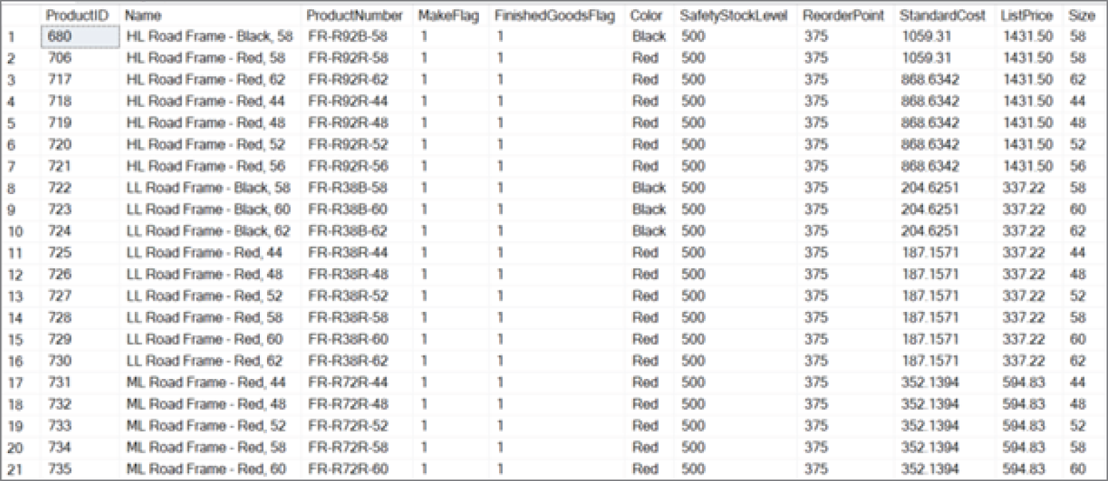
FIGURE 1.5 Structured data
Semi-structured Data
Semi-structured data has some structure to it but no defined schema. This allows data to be written to and read from very quickly since the storage engine does not reorganize the data to meet a rigid format. While the lack of a defined schema naturally eliminates most of the data volatility concerns that come with structured data, it makes analytical queries more complicated as there isn't a reliable schema to use when creating the query.
The most popular examples of semi-structured datasets are XML and JSON files. JSON specifically is very popular for sharing data via a web API. JSON stores data as objects in arrays, which allows an easy transfer of data. Both XML and JSON formats have somewhat of a structure but are flexible enough that some objects may have more or fewer attributes than others. Because the structure of the data is more fluid than that of a database with a schema, we typically refer to querying semi-structured data as schema-on-read. This means that the query definition creates a sort of quasi-schema for the data to fit in. Figure 1.6 demonstrates how JSON can be used to store data for multiple customers while including different fields for each customer.
There are multiple ways that we can store semi-structured data, varying from NoSQL databases such as Azure Cosmos DB (see Chapter 3) to files in an Azure storage account (see Chapter 4). Relational databases such as SQL Server, Azure SQL Database, and Azure Synapse Analytics can also handle semi-structured data with the native JSON and XML data types. While this creates a convenient way for data practitioners to manage structured and semi-structured data in the same location, it is recommended to limit the amount of semi-structured data you store in a relational database to very little or none.
Semi-structured data can also be stored in other types of NoSQL data stores, such as key-value stores, columnar databases, and graph databases.
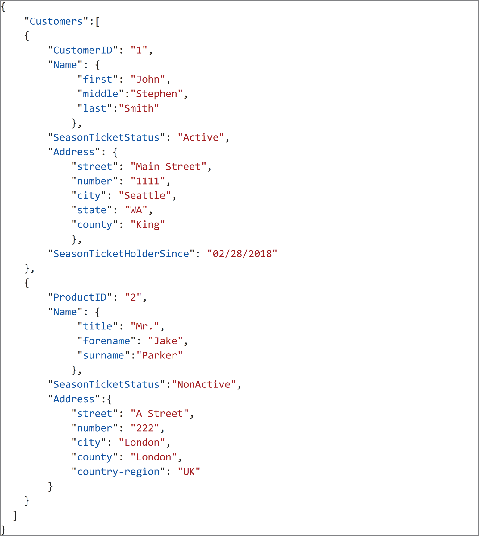
FIGURE 1.6 JSON example
Unstructured Data
Unstructured data is used to describe everything that doesn't fit in the structured or semi-structured classification. PDFs, images, videos, and emails are just a few examples of unstructured data. While it is true that unstructured data cannot be queried like structured or semi-structured data, deep learning and artificial intelligence (AI) applications can derive valuable insights from them. For example, applications using image classification can be trained to find specific details in images by comparing them to other images.
Storing unstructured data is easier today than it has ever been. As mentioned previously, Azure Blob Storage allows companies and individuals the ability to store exabytes of data in any format. While this exam does not cover the many applications of unstructured data, it is important to note that unstructured data is becoming more and more vital for companies to gain a competitive edge in today's world.
Data Velocity
The speed at which data is processed is commonly known as data velocity. Requirements for data processing are largely dependent on what business problem or problems we are trying to solve. Raw data such as football player statistics could be stored as raw data until every game for a given week is finished before it is transformed into insightful information. This type of data processing where data is processed in batches is commonly referred to as batch processing. We can also process data from sensors located on equipment that a player is wearing in real time so that we can monitor player performance as the game is happening. This type of data processing is called stream processing.
Batch Processing
Batch processing is the practice of transforming groups, or batches, of data at a time. This process is also known as processing data at rest. Traditional BI platforms relied on batch processing solutions to create meaningful insights out of their data. Concert venues would leverage technologies such as SQL Server to store batch data and SQL Server Integration Services (SSIS) to transform transactional data on a schedule into information that could be stored in their data warehouse for reporting. Many of the same concepts apply today for batch processing, but cloud computing gives us the scalability to process exponentially more data. Distributed computing paradigms such as Hadoop and Spark allow organizations to use compute from multiple commodity servers to process large amounts of data in batch.
Batch processing is typically done in a process of jobs automated by an orchestration service such as Azure Data Factory (ADF). These jobs can be run one by one, in parallel, or a mix of both depending on the requirements for the solution these jobs are a part of. Automated batch jobs can be run after a certain data threshold is reached in a data store but are more often triggered one of two ways:
- On a recurring schedule—an ADF pipeline running every night at midnight, or on a periodic time interval starting at a specified start time.
- Event/trigger-based—an ADF pipeline running after a file is uploaded to a container in Azure Blob Storage.
It is also critical that batch processing includes error handling logic that acts on a failed job. A common architecture pattern that handles batch processing in Azure is illustrated in Figure 1.7.

FIGURE 1.7 Common architecture for batch processing in Azure
There is quite a bit going on in the diagram in Figure 1.7, so let's break it down step-by-step:
- Data is loaded from disparate source systems into Azure. This could vary from raw files being uploaded to a central data repository such as Azure Data Lake Storage Gen2 (ADLS) to data being collected from business applications in an OLTP database such as Azure SQL Database.
- Raw data is then transformed into a state that is analytics and report ready. Here, we can choose between code-first options such as Azure Databricks to have complete control over how data is transformed or GUI-based technologies such as Azure Data Factory Data Flows. Both options can be executed as activities in an ADF pipeline.
- Aggregated data is loaded into an optimized data store ready for reporting. Depending on the workload and the size of data, an MPP data warehouse such as Azure Synapse Analytics dedicated SQL pool can be used to optimally store data that is used for reporting.
- Data that is ready to be reported is then analyzed through client-native applications or a business intelligence tool such as Power BI.
While the architecture in Figure 1.7 is a common pattern for batch processing data, it is by no means the only one. Deciding on the most appropriate technologies and strategies for processing batch data requires exploratory analysis of the data, knowledge of the source data that will be processed, and well-defined requirements for how the data will be used. You will also need to decide on an extract, transform, and load (ETL) or an extract, load, and transform (ELT) data manipulation pattern, depending on whether your storage and transformation engines are one and the same. The section “Data Processing Techniques” later in this chapter further examines each of these two patterns. Batch processing includes the following advantages:
- Accurately processing large volumes of data at a time. More compute power can be allocated to batch processing, and the time constraint for batch processing usually isn't as critical as it is with stream processing.
- Conveniently scheduling when data is processed. Batch processes can be scheduled whenever, which allows organizations to schedule their batch jobs to run off-peak hours.
- Easily creating complex analytics and aggregations of data. Because the data processed in batches is persisted in data stores such as ADLS, Azure SQL Database, and Azure Synapse Analytics, organizations can return to clean datasets repeatedly for reporting and machine learning purposes.
- Transforming semi-structured data such as JSON or XML data into a structured, schematized format that is ready for analytical queries.
Batch processing includes the following disadvantages:
- Latency between receiving data and being able to analyze it.
- Data that is processed in batch jobs must be ready before the batch can be processed. As mentioned previously, complex error handling checks need to be in place to ensure that problems with data, errors, or failed activities do not bring the entire process down.
Stream Processing
Instead of processing groups of data at scheduled intervals as you would with batch processing, stream processing performs actions on data in real time as it is generated. The proliferation of connected applications and IoT sensor devices in recent years has led to a boom in the amount of data sources that can stream data. Organizations that leverage data streams are able to innovate at an on-the-go pace, allowing them to instantly respond to the needs of their customers.
You can think of a stream of data as a continuous flow of data from some source, also known as a message producer. Each piece of data in a stream is often referred to as an event or a message and typically arrives in an unstructured or semi-structured format such as JSON. The following list includes some examples of stream processing:
- An e-commerce company analyzing click-stream data as consumers are browsing the company's website to provide product recommendations in real time
- Fitness trackers streaming heart rate and movement data to a mobile app and providing real-time updates of the wearer's workout efficiency
- Financial institutions tracking stock market changes in real time and automatically making portfolio decisions as stock prices change
- Oil companies monitoring the status of pipelines and drilling equipment
While these examples include the same transformation activities as many batch processes, they have vastly shorter latency requirements.
Stream processing is just one step in designing a real-time data processing solution. The following logical components will need to be considered when designing a real-time solution:
- Real-time message ingestion—The architecture must include a way to capture and store real-time messages regardless of the technology that is creating the stream of data. Message brokers such as Azure Event Hubs, Azure IoT Hub, and Apache Kafka are used to ingest millions of events per second from one or many message producers. These technologies will then queue messages before sending them to the next appropriate step in the architecture. Most of the time this will be a processing engine of some type, but some solutions will require sending the raw messages to a long-term storage solution such as Azure Blob Storage or ADLS for future batch analysis.
- Stream processing—Stream processing engines are the compute platforms that process, aggregate, and transform data streams. Technologies such as Azure Functions, Azure Stream Analytics, and Azure Databricks Structured Streaming can create time-boxed insights data that is queued in a real-time message broker. These technologies will then write the results to message consumers such as an analytical data store or a reporting tool that can display real-time updates.
- Analytical data store—Processed real-time data can be written to databases such as Azure Synapse Analytics, Azure Data Explorer, and Azure Cosmos DB that power analytical applications.
- Analysis and reporting—Instead of being written to an analytical data store first, processed real-time data can be published directly from the stream processing engine to report applications like Power BI.
Using these steps, we have the flexibility to choose if we want to process data streams live, on demand, or a combination of both. The “live” approach is the most common method for processing data streams and involves analyzing data continuously as it arrives from a message broker such as Azure Event Hubs. This approach is what allows organizations to create calculations and aggregations against data streams for temporal analysis. Figure 1.8 illustrates this approach with a simple example of an IoT-enabled thermostat streaming temperature data to Azure for analysis.

FIGURE 1.8 Live stream processing
This approach produces a real-time streaming solution that creates temperature analysis on the fly while storing the transformed data in an Azure SQL Database for further analysis such as comparing one month's temperature data to the same month in the previous year.
While most streaming solutions will be designed with the live approach, there are some cases that call for processing stream data in micro-batches. This “on-demand” approach involves persisting incoming data into a data store like ADLS and processing the data when convenient. If the scenario does not require real-time analysis, then this can significantly cut computing costs. Figure 1.9 illustrates an example of this approach. While it is like the solution in Figure 1.8, the on-demand design adds an extra step that stores temperature data in ADLS before Azure Stream Analytics performs any computations on the data and outputs it to Power BI and Azure SQL Database.

FIGURE 1.9 On-demand stream processing
Solutions such as this demonstrate how technologies that are typically used for batch processing scenarios can be used in stream processing solutions. In the next section, we will discuss how modern design principles can be used to leverage batch and stream processing in the same solution.
Leveraging Batch and Stream Processing Together
Until recently, most organizations were limited to how quickly they could process data by the hardware and network connectivity in their datacenters. They were often limited to the types of queries they could run with real-time data and were often left waiting for hours on stream processing activities to complete. However, the scalability of cloud-based solutions such as those in Azure empower organizations to process data whenever they want. This flexibility has given way to modern architectural designs that creatively analyze batch- and stream-processed data in the same solution. One of the most popular of these design patterns is the Lambda architecture. The Lambda architecture is a data processing architecture that separates batch and stream processing operations into a cold path and a hot path. Figure 1.10 illustrates the movement of this pattern.

FIGURE 1.10 Lambda architecture
Solutions that use a Lambda architecture create two paths for data processing:
- The cold path is where the batch processing operations, also known as the batch layer, occur. Data flowing into this path is not constrained to low latency requirements, allowing for much larger datasets to be processed on a scheduled basis. Once data has been processed in the batch layer, the results are sent to a serving layer (e.g., data warehouse such as Azure Synapse Analytics or Azure SQL Database) for querying.
- The hot path is where speed processing operations, also known as the speed layer, occur. Data flowing into this path need to be processed as quickly as possible, at the expense of accuracy. Once processed, data from the speed layer either is sent directly to the analytics/report application for analysis or incrementally updates the serving layer based on the most recent data.
Eventually, data from the hot and cold paths will converge at the analytics/report application. If the application needs to display data in real time, it will acquire it from the hot path. Otherwise, the application will read data from the cold path to display more accurate analysis created from a larger dataset.
One of the core principles of the Lambda architecture is that raw data stored in the batch layer is immutable. New data is always appended to existing data, never overwriting older data. Changes to the value of a particular dataset are stored as a new time-stamped record. This allows for recompilation of computations at any point in time to provide more accurate historical analysis. Azure enables organizations to easily implement this design without needing to purchase and install new hardware. For example, Azure Data Lake Storage Gen2 can store petabytes worth of information, and with its native hierarchical namespaces (think of directories and folders in a file explorer), organizations can create directory trees corresponding to different dates that can store and maintain data that was generated on that date. Organizations are not burdened with scaling existing or installing new storage devices and can instead focus on implementing business logic.
Describe Data Analytics Core Concepts
The process of taking raw data and turning it into useful information is known as data analytics. Companies that invest in sophisticated, well-designed data analytics solutions do so to discover information that helps the overall performance of the organization. Finding new opportunities, identifying weaknesses, and improving customer satisfaction are all results that come from data analytics. This involves building a repeatable solution that collects data from the appropriate source systems, transforms it into dependable information, and serves it in a way that is easy to consume.
One example of an end-to-end data analytics solution is a sports franchise that would like to build a fan engagement solution to improve stadium attendance rates and in-stadium retail sales by retaining more season ticketholders and creating incentive-based programs for different fan groups. The first step to create this solution will be to identify the sources of data that will be most useful to answering questions related to who attends games and what external factors may influence attendance rates. The next step will be to take these disparate sources of data and transform them so that they present a reliable view of the data that can be easily read by consumers who are acting on the data. For example, consumers of the data could be data scientists who develop regression models that predict future stadium attendance or analysts who build reports and dashboards that display in-stadium trends for different fan groups. These actions are then used to create decisions that will enhance ticket sales and operational efficiency during a game.
Data Processing Techniques
The most critical part of a data analytics solution is that the result set is clean, reliable data. Consumers of the data must be able to retrieve the same answer from a question, regardless of how the question is presented to the data model. There cannot be a question of the quality of data being reported on. This is the goal of data processing.
Simply put, data processing is the methodology used to ingest raw data and transform it into one or more informative business models. Data processing solutions will ingest data either in batches or as a stream and can either store the data in its raw form or begin transforming it. Data can undergo several transformations before it is ready to be reported on. Some of the most common transformation activities are as follows:
- Filtering out corrupt, duplicated, or unnecessary data
- Joining data or appending it to other datasets
- Normalizing data to meet a standard nomenclature
- Aggregating data to produce summarizations
- Updating features to a more useful data type
Data processing pipelines must include activities that are repeatable and flexible enough to handle a variety of scenarios. Tools such as ADF, Azure Databricks, and Azure Functions can be used to build processing pipelines that use parameters to produce desired results. These tools also allow developers to include error handling logic in their processing pipelines to manage how pipelines proceed if processing errors present themselves without bringing the pipeline to a screeching halt.
Cloud-based data processing solutions make it easy to store data after multiple stages of transformations. Storage solutions such as ADLS allow organizations to store massive amounts of data very cheaply in folders designated for raw data that was just ingested, data that has been filtered and normalized, and data that has been summarized and modeled for reporting. This allows data processing solutions to reuse data at any point in time to validate actions taken on the data and produce new analysis from any point in the data's life cycle.
There are two data processing approaches that can be taken when extracting data from source systems, transforming it, and loading the processed information into a data model. These approaches are extract, transform, and load (ETL) and extract, load, and transform (ELT). Choosing between them depends on the dependency between the transformation and storage engines.
Extract, Transform, and Load (ETL)
ETL pipelines process data in a linear fashion with a different step for each phase. They first collect data from different sources, transform the data to remove dirty data and conform to business rules, and load the processed data into a destination data store. This approach has been used in business intelligence (BI) solutions for years and has a wide array of established best practices. Each of the three phases requires an equal amount of attention when being designed. If properly designed and developed, ETL pipelines can process multiple sources of data in parallel to save time. For example, while data from one source is being extracted, a transformation activity could be working on data that has already been received, and a loading process can begin working on writing the transformed data to a destination data store such as a data warehouse. Figure 1.11 illustrates common Azure technologies used in each phase of an ETL workflow.

FIGURE 1.11 ETL workflow
In this example, data is extracted from its source systems and transformed by one or more compute engines such as Azure Databricks, Azure Functions, or Azure Data Factory mapping data flows. After the necessary transformations are completed, the data is loaded into a destination data store such as Azure Synapse Analytics, Azure Cosmos DB, ADLS, or Azure SQL Database to power different types of applications. ADF automates this workflow and controls when each step is executed. Keep in mind that this is a rudimentary example and a typical ETL pipeline may include several staging layers and transformation activities as data is prepared. The following sections describe each phase and how each activity is managed in an ETL workflow.
Extract
The first phase of an ETL process involves extracting data from different source systems and storing it in a consolidated staging layer that is easier for the transformation tools to access. Data sources are typically heterogenous and are represented by a wide variety of data formats. The staging layer can be transient to cut back on storage demands or to eliminate personally identifiable information (PII) that may be present in the source systems or persisted if PII data is not present and storage is not a concern. The staging layer is typically persisted as files in an object store such as Azure Blob Storage or ADLS.
In Azure, tools such as Azure Logic Apps and ADF allow data engineers to drag and drop activities with a graphical user interface (GUI) that copies data from source systems and land them in the staging layer. These activities can be parameterized to dynamically adjust where the raw data is staged. Custom code options such as Azure Databricks and Azure Functions are also available to extract data with languages such as C#, Python, Scala, and JavaScript. The very nature of these custom code options gives data engineers more control over how extracted data is formatted and staged. Regardless of whether data extraction is done with a GUI-based or code-first tool, data extraction activities can be automated to run on a schedule or event driven based on when new data is added to the source system.
Data can be extracted from a source system a few different ways. Incremental extractions involve only pulling source data that has been recently inserted or updated. This can minimize both the time to extract the necessary source data and the time to transform the new raw records but requires additional logic to determine what data has been changed. For systems that are not capable of identifying which records have changed, a full data extraction needs to take place. This requires having a full copy of the source data being extracted. While that can result in an accurate copy of the source data, it could take longer to extract, and subsequent transformation activities will take longer to run.
Transform
The second phase of an ETL process involves transforming the extracted data that is cleansed and meets a set of business requirements. Data is scrubbed of dirty data and prepared so that it fits the schema of the destination data model. Transformations are split into multiple activities for optimal data pipeline performance. This modular approach allows transformation activities to run in parallel and provides an easier method for troubleshooting failed tasks. It also allows data engineers to easily implement additional transformation activities as new business requirements are added.
Depending on the complexity of the transformations, data may be loaded into one or more additional staging layers to serve as intermediary stages for partially transformed data. One example of this is splitting the different phases of data transformations into bronze, silver, and gold staging layers.
- The bronze layer represents raw data ingested from different sources in a variety of different formats. Some filtering may have happened to get the data to this stage, but there are minimal transformations to data in the bronze layer.
- The silver layer represents a more refined view of the data. Silver layer data is characterized by data that has been scrubbed of dirty records and entities made up of fields from multiple bronze layer datasets using join or merge operations. Data in the silver layer is typically used for machine learning activities since this data is cleansed but not summarized.
- The gold layer represents aggregated datasets that are used by reporting applications. Calculations such as weekly sales and month-over-month averages are included in gold layer datasets.
As in the extract phase, transformation activities can be built with GUI-based or code-based technologies. SQL Server Integration Services (SSIS) is an ETL tool that is involved in traditional, on-premises BI solutions. SSIS provides many connectors and transformation activities out of the box that allow developers to build sophisticated data engineering pipelines with a GUI. ADF provides a similar development experience for cloud-based ETL. ADF provides a drag-and-drop experience with several data transformation activities out of the box that can be chained together graphically. The core components of how ADF orchestrates ETL pipelines will be discussed in the section “Control Flows and Data Flows” later in this chapter, but as far as transformations are concerned, ADF can execute transformation activities in four ways:
- External Compute Services—ADF can be used to automate the execution of externally hosted transformation activities that are custom coded. These activities can be developed in several different languages and hosted on tools such as Azure Databricks and Azure Functions. Stored procedures hosted on Azure SQL Database or Azure Synapse Analytics can also be invoked by ADF using the Stored Procedure Activity. Transformations that are developed from scratch give engineers more flexibility on how to implement business rules and how to handle different scenarios. ADF allows engineers to pass results from previous steps in a data pipeline as parameters or static predefined parameters to a custom-developed transformation activity so that it can transform data more dynamically.
- Mapping Data Flows—ADF gives data engineers the option to build no-code transformation pipelines with the use of mapping data flows. These are very similar to data flow activities in SSIS, giving data engineers the ability to create transformation activities with a GUI. The benefit of a no-code solution like this is that the code performing the transformations and the compute running the code is obfuscated from the data engineer. This can greatly improve operational productivity by allowing engineers to purely focus on implementing business logic instead of optimizing code and compute infrastructure. Just as with transformation activities that are hosted on external compute services, ADF can pass static parameters or results from previously executed activities as parameters to mapping data flows to dynamically transform data.
- Power Query—Previously known as wrangling data flows, ADF allows data engineers to perform no-code transformations on data using Power Query. Power Query is a native component of Power BI and gives analysts the ability to perform transformation activities in a scalable manner. Power Query in ADF enables citizen data analysts to create their own pipelines in ADF without needing to know how to build sophisticated data engineering pipelines.
- SSIS—Organizations have been building BI solutions for many years now, and if their solution involved SQL Server, then there is probably an SSIS component involved. Rebuilding existing SSIS with ADF pipelines could be very time consuming if the existing SSIS footprint is sophisticated. This can be a blocker for organizations migrating to Azure. To alleviate these concerns, customers can choose to migrate their SSIS projects to ADF. Data engineers can use the Execute SSIS Package activity in their data pipelines as singleton activities or chained to other ADF native activities. Running an SSIS project in ADF requires the use of a special compute infrastructure known as the Azure-SSIS integration runtime to run them. Chapter 5 will discuss the Azure-SSIS integration runtime and other types of runtimes in further detail.
Load
The last phase of an ETL process involves loading the transformed data to a destination data model. This data model can be a data warehouse such as Azure Synapse Analytics or Azure SQL Database, a database such as Azure Cosmos DB that serves highly distributed web applications, or an object store such as ADLS that is used as the golden copy of data for machine learning activities. This phase can also be handled by GUI-based tools such as ADF or custom code solutions.
Data can be loaded to a destination data store using a few different loading patterns. Incremental or differential loads involve adding new data or updating existing data with new values. This can reduce the amount of time it takes to load newly transformed data to the destination data store, allowing consumers of the data to analyze the new data as quickly as possible. Sometimes there is a need to load the destination data store with the entire dataset, requiring an erasure of the existing data store's data. For these use cases, it can be useful to have a staging table in the destination data store to serve as an intermediary between the final transformed copy of the data and production tables being analyzed. Since the staging tables are the tables being truncated, consumers would not experience any downtime from missing data. New records can be added to the production table through a process called partition switching.
Relational database tables that are loaded with data processed by an ETL pipeline must have their schemas prebuilt. Not considering the structure of a table's existing schema can result in load errors stemming from mismatched data types and incorrect column names. This requirement to shape data so that it conforms to a predefined schema is known as schema-on-write.
Control Flows and Data Flows
Many ETL tools employ two methods for orchestrating data pipelines. Tasks that ensure the orderly processing of data processing activities are known as control flows. Data processing activities are referred to as data flows and can be executed in sequence from a control flow. Data engineers that use ADF to orchestrate their data pipelines can use control flows to manage the processing sequence of their data flows.
Control flows are used to enforce the correct processing order of data movement and data transformation activities. Using precedence constraints, control flows can dictate how pipelines proceed if a task succeeds or fails. Subsequent tasks do not begin processing until their predecessors complete. Examples of control flow operations in ADF include Filter, ForEach, If Condition, Set Variable, Until, Web, and Wait activities. ADF also allows engineers to run entire pipelines within a pipeline after an activity has finished with the Execute Pipeline control flow activity. Figure 1.12 shows a simple control flow in ADF, where the Lookup task is retrieving table metadata from a SQL Server database that will be passed to a set of Copy activities to migrate those tables to a data warehouse hosted in Azure Synapse Analytics.

FIGURE 1.12 ADF control flow
This control flow includes outcomes for successful lookups of table metadata and failures. If metadata is retrieved successfully, then the next step will be a ForEach loop that includes data movement tasks that will migrate each SQL Server table successfully retrieved to Azure Synapse Analytics. If the Lookup task fails for whatever reason, then the next step will be a Web activity that will send an email alerting an administrator of the failure.
Another example of a control flow is the order in which different mapping data flows are executed. Using the Data Flow activity, data engineers can chain together multiple mapping data flows to process data in the correct order. Figure 1.13 illustrates an example of a control flow that executes a series of data flows sequentially and in parallel.

FIGURE 1.13 Ordering data flow processing with a control flow
This pipeline begins by inserting new State fields followed by new geography fields in the State and geography destination tables, all the while inserting new specialty fields in parallel. Once these data flows are complete, the control flow will run a final data flow that inserts new detail fields into the destination detail table. Of course, these tasks only control what order ETL activities run in, not the underlying data transformation steps. ADF allows developers to build or edit specific mapping data flows by double-clicking their corresponding Data Flow control flow activity.
While control flows manage the order of operations for ETL pipelines, data flows are where the ETL magic happens. Data flows are specific tasks in a control flow and are responsible for extracting data from its source, transforming it, and loading the transformed data into the appropriate destination data stores. The output of one data flow task can be the input to the next one, and data flows without a dependency on each other can run in parallel. As mentioned in the section “Transform” earlier in this chapter, ADF can execute four types of transformation activities that can serve as data flows. This section will focus on two of those types: mapping data flows and external compute services that host custom code.
Mapping data flows are ETL pipelines that data engineers can design with a GUI. Developers begin by selecting a source to extract data from, then performing one or more transformation activities on the data, and finally loading the transformed data into a destination data store. The finished data flows are translated to code upon execution and use scaled-out Apache Spark clusters to run them. Figure 1.14 is a screenshot of the Insert New DimSpecialty fields data flow task from Figure 1.13.

FIGURE 1.14 ADF mapping data flow
This data flow begins by extracting data from a CSV file. Next, the CSV data undergoes a few transformations including the removal of duplicate rows, selecting only the columns needed, and creating new columns to conform to the destination data store's schema. Finally, the data flow loads the transformed data to the DimSpecialty table in Azure Synapse Analytics by inserting each transformed column into its associated destination column. Once these tasks are completed, the control flow will flag this data flow as being successfully completed and wait on the Insert New DimGeography Fields data flow to successfully complete before moving on to the Insert New FactDetail Values data flow.
ADF can also be used to automate custom-coded data flow activities that are hosted in external compute services such as Azure Functions, Azure Databricks, SQL Stored Procedures, or Azure HDInsight. Code hosted on these platforms can be used to perform one or more phases of an ETL pipeline. Running these tasks as activities in ADF allows them to run on a scheduled basis and alongside other activities such as mapping data flows or other custom-coded data flows. Figure 1.15 illustrates a control flow in ADF that executes external data flows that are hosted in Azure Databricks and Azure SQL Database.

FIGURE 1.15 Azure Databricks and SQL stored procedure control flow
This example is a part of a solution that analyzes American football players who are NFL football players. The destination data store is a data warehouse hosted on an Azure SQL Database that provides consumers with the ability to compare the current year's group of prospects with those in previous years. The pipeline in Figure 1.15 starts by running a Python notebook hosted in Azure Databricks that extracts information on when a prospect was selected in the current year's NFL Draft, cleanses the data, and loads the cleansed data in the data warehouse. The next step in the pipeline is to run a stored procedure in the data warehouse that associates a unique identifier that was assigned to them before the NFL draft. Finally, the pipeline executes another stored procedure that tells analysts if a prospect was not drafted. As you can see, each of these data flows is critical to the success of this data analytics solution. ADF makes it possible to run these activities that are developed on different technologies in sequential order and control when they should run.
Extract, Load, and Transform (ELT)
ELT workflows differ from ETL workflows solely in where the data transformation takes place. Instead of a separate transformation engine, the destination data store is used to load and transform data. This simplifies the design by removing extraneous components that would typically be used to transform data. Since the transformation and load components are one and the same, the destination data store must be powerful enough to efficiently complete both tasks at the same time. This makes large-scale analytics scenarios the perfect use cases for ELT workflows since they rely on the scalability of MPP technologies such as Azure Synapse Analytics or Azure Databricks. Figure 1.16 illustrates the common Azure technologies used in each phase of an ELT workflow.

FIGURE 1.16 ELT workflow
In this example, data is extracted from its source systems via ADF and stored as flat files in a raw data store such as ADLS or Azure Blob Storage. Next, data is virtually “loaded” into staging tables in the destination data store. Data virtualization is what enables ELT workflows to process massive amounts of data with relatively little overhead. Instead of data being physically stored in the destination data store, external tables are used to overlay a schema over the flat file data in ADLS or Azure Blob Storage. The data is then able to be queried like any other table, without taking up storage in the destination data store. MPP technologies such as Spark (using Azure Databricks or Azure Synapse Apache Spark pools) and Azure Synapse Analytics are typical data stores used for this approach because they have mechanisms for creating external tables and performing transformations on them. The following sections will describe each phase in further detail.
Extract
Collecting data from various sources is just as important in ELT workflows as it is in ETL. Unlike with ETL scenarios that might begin raw processing once the data is extracted, data involved in ELT scenarios is always consolidated in a central repository. These repositories must be able to handle large volumes of data. Scalable file systems that are based on the Hadoop Distributed File System (HDFS), such as ADLS and Azure Blob Storage, are typically used in these scenarios.
Extracted data must also be in formats that are compatible with the loading mechanisms of the destination technology. Typical file formats include delimited text files, such as CSV or TSV, semi-structured files such as XML or JSON, and column compressed files such as AVRO, ORC, or Parquet. Column compressed file formats should be used for larger datasets as these are optimized for big data workloads because they support very efficient compression and encoding schemes. Parquet is widely used because of its ability to embed the data's schema within the structure of the data, thus reducing the complexity of data loading and transformation logic.
Load and Transform
The key to any ELT workflow is the destination data store's ability to process data without needing to store it in-engine. MPP technologies do this by fitting a schema over one or more files that are stored in ADLS or Azure Blob Storage. The destination data store only manages the schema of the data and not the storage of it. These external tables allow engineers to query and process data as they would a table that is stored in the destination data store but minimizes the amount of storage required by it. Transformations that are performed on the virtualized data take advantage of the features and capabilities of the destination data store but are applied to the data in object storage.
The three Azure technologies that can perform load & transform operations in an ELT workflow are Azure HDInsight, Azure Databricks, and Azure Synapse Analytics.
- Azure HDInsight is a managed cloud service that lets data engineers build and manage Hadoop, Spark, Kafka, Storm, and HBase clusters that can process stored data in ADLS or Azure Blob Storage. HDInsight clusters use Apache Hive to project a schema on data in object storage without needing to persist the data locally on the cluster. This decoupling of compute from storage allows clusters to process data at scale.
- Azure Databricks is a fully managed, cloud-based data platform that allows data engineers to build enterprise-grade Spark-powered applications. Databricks was built by the same team that built Apache Spark and provides a highly optimized version of the open-source version of the Spark runtime. Azure Databricks is a specific implementation of Databricks that includes native integration with a variety of Azure-based storage such as ADLS, Azure Blob Storage, Azure Synapse Analytics, Azure SQL Database, and Azure Cosmos DB. Azure Databricks provides a similar mechanism to decoupling compute from storage as Azure HDInsight but has a few key advantages. For one, Azure Databricks provides native integration with Azure Active Directory for identity and access management. Azure Databricks also provides easier ways to manage clusters by letting data engineers manually pause clusters or set an auto-shutdown after being idle for a fixed amount of time. Clusters can also be set to auto-scale to support different workload sizes.
- Azure Synapse Analytics is a comprehensive data analytics platform that includes tools for data ingestion, transformation, exploration, and presentation. For the purposes of this section, we will focus on the three tools that can be used for the load and transform phases: dedicated SQL pools, serverless SQL pools, and Apache Spark pools.
- Dedicated SQL pools, formerly known as Azure SQL Data Warehouse, store data in relational tables with columnar storage. A dedicated SQL pool can scale up or down depending on how large the workload is and can be paused when it's not being used. Data engineers can choose to virtualize data that is stored in object storage with either PolyBase or the COPY statement. PolyBase uses external tables to define and access the data in Azure object storage. PolyBase requires the creation of a few external objects to be able to read data. These include an external data source that points to the data's location in either ADLS or Azure Blob Storage, an external file format that defines how the data is formatted, and finally the actual external table definition. The COPY statement is a newer command for loading data into a dedicated SQL pool. It simplifies the load process by requiring only a single T-SQL statement that needs to be run instead of needing to create multiple database objects. It also includes some additional features to what PolyBase offers. Going forward, the COPY statement should be used to load data from ADLS and Azure Blob Storage to a dedicated SQL pool.
- Serverless SQL pool is an interactive service that allows developers to query data in ADLS or Azure Blob Storage. It is a distributed data processing system, built for large-scale data explorations. There is no infrastructure to set up or clusters to maintain since it is serverless. A default endpoint for a serverless SQL pool is provisioned for every Azure Synapse Analytics workspace that is deployed. Data engineers and data analysts can use the OPENROWSET function to query files in Azure object storage and can create external tables or views to maintain the structure of the data for later usage. Serverless SQL pools support T-SQL for users querying and processing data.
- Apache Spark pools allow data engineers to deploy Spark clusters using the open-source version of Spark to process large volumes of data.
Each of these technologies is an MPP system and is designed to handle big data scenarios. The key advantage of using an MPP technology like the ones just discussed for big data scenarios is that once the data is loaded, they will break the data down into smaller partitions and distribute the processing of the partitions across multiple machines in parallel. Instead of one job processing a mammoth sized dataset, transformations can occur in parallel on smaller subsets of the data, resulting in more efficient processing of the data. For more information on Azure HDInsight, Azure Databricks, and Azure Synapse Analytics and to better understand when to use which one or how to use them in tandem, see Chapter 5.
Describe Analytics Techniques
While it is important to spend considerable time planning and developing data processing pipelines, it is vital not to forget about the questions that drove the solution to be built in the first place. Being able to answer questions like the following is critical to the success of a business: What has happened? Why did certain events happen? What will happen? What should we do? and What might happen if different variables change?. Knowing how to answer these questions can help businesses understand their past successes and failures and predict what actions they should take in the future. These questions can be answered using the five types of analytics techniques, telling the story of a business's past, present, and future.
The five types of analytics include descriptive, diagnostic, predictive, prescriptive, and cognitive analytics. Each type of analytics represents a different stage of an organization's analytics maturity. For example, descriptive analytics techniques are based on decades of best practices that are easier to implement than prescriptive analytics but do not provide as much value. The relationship between the value provided by an analytics technique and its implementation complexity is known as the Analytics Maturity Model. This is illustrated in Figure 1.17.

FIGURE 1.17 Analytics Maturity Model
Descriptive
Descriptive analytics use historical data to answer questions about what has happened to the business. This is a great first step for conducting statistical analysis as it informs decision makers of any trends, data distribution, and if there are any outliers in the data. Key performance indicators (KPIs) allow analysts to summarize large datasets to track the success and failure of key objectives. This type of analysis is reactive and is typically the first analysis technique used by organizations making decisions based on data.
Data used for descriptive analytics is typically gathered and persisted in a central repository, such as a data warehouse. Well-designed data warehouses make it easy for OLAP models and BI tools to analyze performance metrics against a variety of scenarios. An example of descriptive analytics is generating reports to provide a view of an organization's sales data.
Diagnostic
Diagnostic analytics use historical data to answer questions about why different events have happened. While descriptive analytics use historical data to display past results, diagnostic analytics take this a step further by determining the root cause behind those results. This is the first technique that leverages machine learning to provide insights. Examples of diagnostic analytics include drilling down to focus on a particular facet of data, anomaly detection, data mining to get information from a massive set of data, and correlation analysis to pinpoint cause-and-effect relationships.
Predictive
Predictive analytics use historical data to build statistical and machine learning models to forecast what will happen in the future. This is the first type of analytics in the Analytics Maturity Model that answers questions regarding a business's future. Techniques such as neural networks, decision trees, and regression models allow predictive analytics solutions to make recommendations on the following scenarios:
- Whether or not a customer will leave for a competitor. Customer churn models use past trends to make predictions on the risk of a customer leaving. These models can help organizations make decisions on how to preemptively maintain high-risk customers' business.
- When to replace or repair a piece of equipment. Predictive maintenance models enable organizations that rely on machines to run their business (e.g., oil and gas companies or vending machine companies) to know when they should take proactive measures to repair or replace equipment.
- Whether or not a piece of data is fraudulent. Fraud detection models will alert organizations if they find any suspicious transaction activity.
While descriptive and diagnostic analysis can be completed using traditional BI techniques, predictive analysis requires developers to have a more specialized skillset. Along with the need to properly maintain the historical data warehouse, solutions involving predictive analytics must maintain and regularly revisit model performance to ensure that the models are making well-informed decisions. While not in scope for this book, it is important to understand the tools and mechanisms used to maintain a machine learning model's life cycle. Azure Machine Learning and Apache Spark's MLflow enable data scientists to train, deploy, automate, and manage their machine learning models. These technologies allow data scientists to deploy models using container-based technologies such as Kubernetes or Azure Container Instances, which can be used by applications to make batch or real-time predictions.
Prescriptive
Prescriptive analytics solutions are a step up from predictive analytics as they not only predict outcomes, but they also advise organizations on how to reach a desired outcome. These solutions use findings from descriptive, diagnostic, and predictive analytics techniques to answer questions about what actions should be taken to achieve a particular goal. Combinations of machine learning algorithms and business rules are used to simulate the outcomes of different input parameters. One example of the impact prescriptive analytics solutions can make is in the sports science field. Prescriptive analytics solutions not only predict when an athlete will experience a soft tissue injury but will also advise team doctors on what measures to take to prevent them. They can also be used to advise athletes on the most efficient training exercises for performing at their peak.
Cognitive
Cognitive analytics solutions combine several artificial intelligence and machine learning techniques such as deep learning and natural language processing to draw inferences from existing data and patterns. This type of analytics will provide information based on existing knowledge bases and then add this information back into the knowledge base for future inferences.
This type of analytics takes inspiration from the way the human brain processes information. Instead of retrieving data via a query or creating analysis using structured development methods, cognitive analytics solutions are developed to derive more accurate inferences over time by learning from each interaction with data.
Describe Data Visualization Techniques
Different analytics techniques provide a business with the information needed to make critical decisions moving forward but can be difficult to interpret if the findings are left as plain numbers. Data visualization refers to the process of graphically representing valuable information. The resulting infographics include charts, graphs, maps, and other objects that make information easy to read. Visualizations make it easy for analysts and business decision makers to see trends, outliers, and patterns in data. It is for this reason that using the most effective visualizations to represent information is critical to the storytelling process of data analytics.
Data visualization techniques come in a few different flavors. Depending on the purpose of the infographic and the skillset of the end users, data visualizations may be developed using one of the following three methods:
- Analytical tools allow users the ability to access and manipulate very granular levels of data. Tools like SQL Server Analysis Services (SSAS), Azure Analysis Services (AAS), and Power BI store data as OLAP models that can be filtered in a way that allow analysts to view calculated metrics for different scenarios. Data scientists can use tools such as Jupyter Notebooks to develop visualizations in a browser-based shell using Python or R. Using Python or R packages such as matplotlib or ggplot2, data scientists can build visualizations that are highly customized depending on what story they are trying to tell. Analysts and developers building infographics with analytical tools must have an intimate knowledge of the data that they are working with and must possess very specialized development skills. However, while analytical tools require the most complex set of skills to use, they provide users with the most flexibility in how they visualize information.
- Reporting tools give analysts the ability to organize data into informational summaries to monitor how different areas of the organization are performing. Traditional report tools such as SQL Server Reporting Services (SSRS) allow report builders to build static reports that use set filters to monitor business performance, only updating the displayed data when the dataset powering the report is refreshed. Modern technologies such as Power BI improve reporting capabilities by allowing users to dynamically alter the displayed data with filters, slicers, and interactive visualizations. This interactive capability empowers decision makers to consider multiple scenarios when determining the most appropriate course of action for their business. Reports are typically accessed by end users through an online portal such as
powerbi.comand are only accessible to users with the appropriate level of access. You can learn more about Power BI security in Chapter 6, “Reporting with Power BI.” - Dashboarding tools provide quick overviews of the most relevant pieces of information. Dashboards are designed to be easy to consume, allowing decision makers to act shortly after the data exposes new opportunities or threats. Tools such as Power BI allow analysts to collect the most relevant parts of a report to a decision maker and pin them to a dashboard.
Once a decision has been made on the most useful data visualization technique, it is important to choose the visual or visuals most appropriately suited for the data being displayed. Poorly chosen visuals can be hard to interpret or, worse, convey the wrong message. Another important aspect is the design of each visual. It's not enough to choose the correct chart or graph for the job, analysts must also be consistent with the aspect and color scheme for their visuals. This will help keep end users focused on any insights that are displayed rather than being overwhelmed by clashing color patterns and inconsistent sizing. End users should be able to quickly interpret the message each visual is telling with little to no explanation. The following sections include common visualizations used in analytical, reporting, and dashboarding tools. While these visualizations are popular and easy to build, there are countless more available for storytelling.
Table
A table is a grid that contains data that is ordered in rows and columns. Tables work well with quantitative comparisons where you are evaluating many values for a single category. Technologies such as Power BI Paginated Reports and SSRS format large tables to fit onto multiple pages make them easier to read. This type of reporting is known as paginated and has been used in BI solutions for decades. Figure 1.18 is an example of a table that lists the quantity sold and total sales amount for different bike subcategories sold online in different US regions.

FIGURE 1.18 Table
Matrix
A matrix is a table that summarizes data into totals and subtotals for different groupings. In Figure 1.18 we can see that most bikes that are sold online in the United States are sold in the Northwest and Southwest sales territory regions. However, tables can become very hard to read if we start adding additional levels of granularity such as sales data for specific types of bikes. Matrices take care of this issue by providing a hierarchical structure that provides totals for multiple layers of granularity. Figure 1.19 is an example of a matrix that displays order quantity and sales totals for bikes, each bike subcategory, and each specific bike type sold online in the US Northwest and Southwest regions.
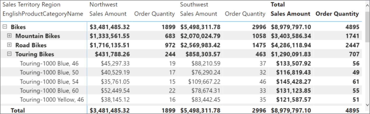
FIGURE 1.19 Matrix
Column and Bar Charts
Bar and column charts enable organizations to see how a set of variables change across different categories. Both chart types represent data with rectangular bars. The difference between the two is that if the rectangles are stacked horizontally, it is called a bar chart, and when they are aligned vertically, then it is a column chart. Figure 1.20 illustrates an example of a column chart that compares the total Internet sales amount for the different subcategories of bikes sold in the US Northwest and Southwest sales territories.

FIGURE 1.20 Column chart
Line Chart
Line charts represent how a series of values change over time. Power BI enhances line charts by including a tooltip that provides more granular information for each data point on the x-axis. This is helpful if you are trying to prove a correlation between data points. Tooltips can be displayed by hovering your mouse over the x-axis value you would like to further analyze. Figure 1.21 illustrates an example of a line chart that compares monthly Internet bike sales in 2011, 2012, and 2013 in the US West sales territory. This line chart also includes a tooltip displaying the Internet sales totals for the month of July in each year.
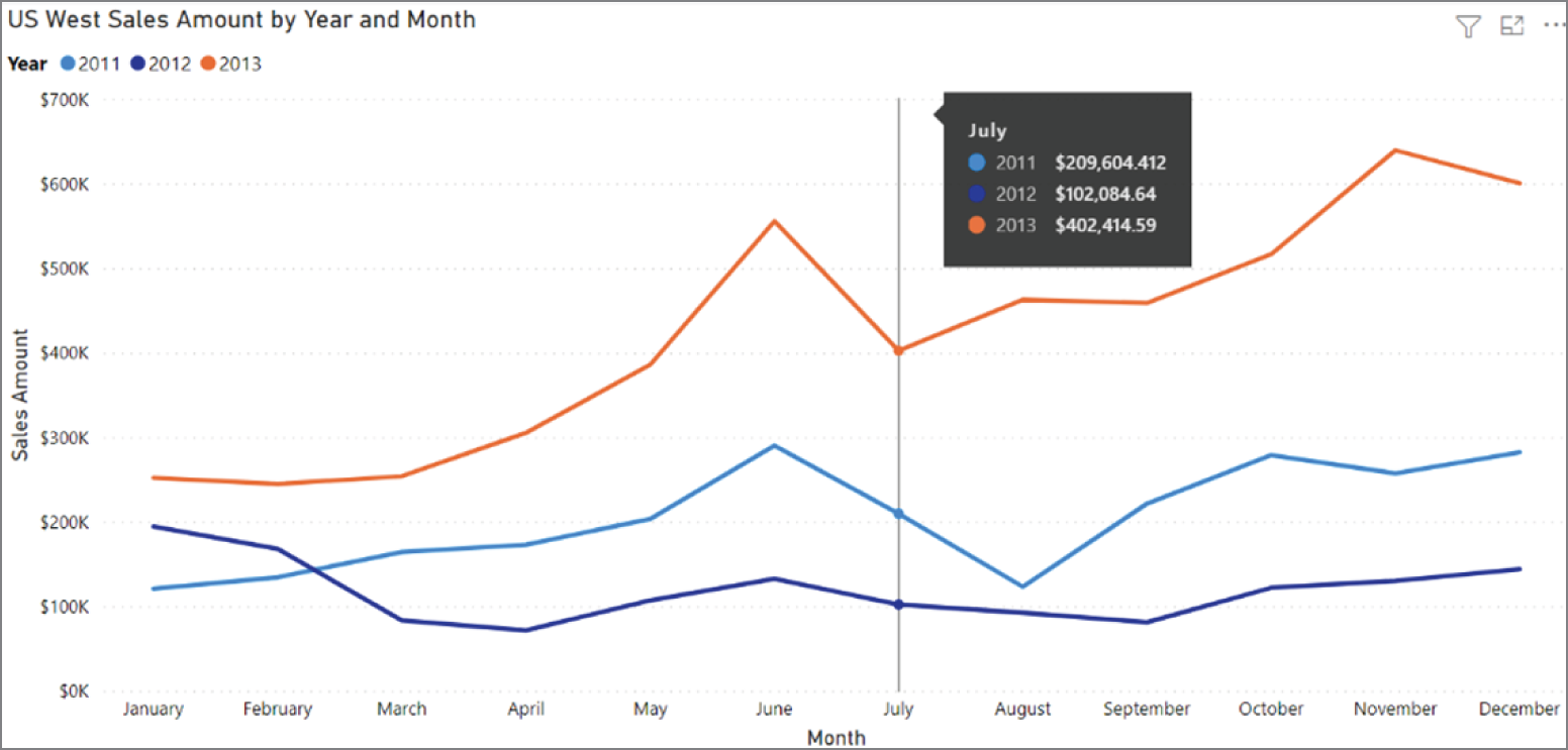
FIGURE 1.21 Line chart
Pie Chart
Pie charts are useful for determining how responsible different categories are for a given value. Each category corresponds to a single slice of the pie, and the size of each slice indicates the percentage of the whole pie each category is responsible for. Figure 1.22 illustrates an example of a pie chart that displays the total Internet bike sales for each country where a sale occurred as well as the percentage of the total sales that each country is responsible for.
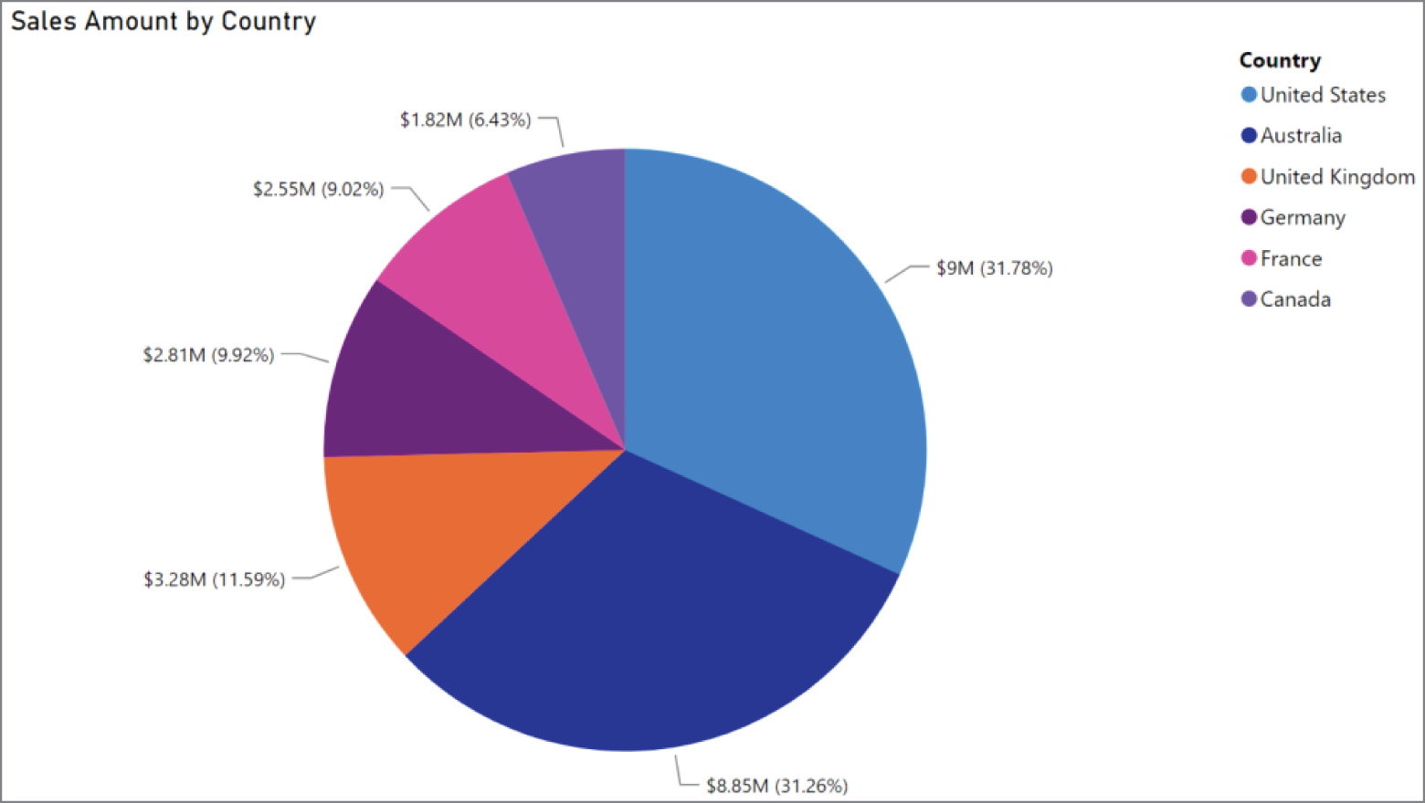
FIGURE 1.22 Pie chart
Scatter Plot
Scatter plots show the relationship between two numerical values. Power BI enhances scatter plots by including a tooltip that provides more granular information for each data point, or bubble. Tooltips can be displayed by hovering your mouse over the bubble you would like to further analyze. Figure 1.23 illustrates a simple example of a scatter plot chart that displays the correlation between the sales amount and order quantity for the different types of bikes sold online. The plot takes the analysis a step further by examining this correlation for the US Northwest and Southwest regions.

FIGURE 1.23 Scatter plot
Map
Maps show the geographic distribution of data. These visualizations can show broad comparisons such as country or state sales information or very granular comparisons at the postal code, address, or latitude and longitude level. Figure 1.24 illustrates a map that displays cities in the US Pacific Northwest where bikes were bought online. The size of the bubble represents the total bike sales proportion that each city is responsible for.

FIGURE 1.24 Map
Summary
The concepts included in this chapter cover the different categories of data, storage options, and processing patterns. This chapter also covered common analysis techniques and when to use different visualizations depending on what business questions you are trying to answer. Understanding these core definitions will help you design data solutions in Azure for any scenario.
This chapter covered the following concepts:
- Describe types of core data workloads. The design strategy for a data solution comes down to what value will be provided by the solution, the volume of data the solution will store and process, the variety of data involved, and the velocity of the data being ingested. Solutions can be either a transactional workload, accounting for the business transactions that support the day-to-day operations of an organization, or an analytical workload that supports business users who need to make calculated business decisions from large amounts of data. These workloads can consist of structured, semi-structured, and unstructured data that can be stored in relational or nonrelational databases or as files in object storage. Cloud-based solutions can easily support requirements for data to be batch and stream processed.
- Describe data analytics core concepts. Data analytics is the process of turning raw data into information that is used to make important business decisions. First, raw data is extracted from source systems that are used to power a business and is either transformed first and then loaded into a destination data store or is loaded first and then transformed in the destination data store. Depending on the value being derived from the information, one or more analytics techniques can be applied to the processed data to view past performance and predict the most optimal actions to take advantage of future opportunities or prevent potential threats. Value is then exposed through several data visualization techniques so that decision makers can easily interpret the processed data and quickly make decisions that will ensure the success of their business.
Exam Essentials
- Describe the characteristics of relational data. Relational databases are data storage technologies that organize data into tables that can be linked based on data common to each other. Database tables store data as rows and are organized into a set number of columns. Relationships between tables allow users to easily query data from multiple tables at the same time. These databases also enforce schema integrity and maintain ACID rules, which makes them a good option for storing structured data. Relational databases are also critical for analytical workloads such as data warehouses because they structure data in a way that is easy to serve to reporting applications.
- Describe the characteristics of nonrelational data. Nonrelational data is data that requires flexibility in the way it is stored. Semi-structured data such as JSON and XML and unstructured data such as images or videos are some examples of nonrelational data. NoSQL databases can be used to store data with constantly changing schemas without forcing it to conform to a fixed structure. This allows queries that write and read data from these databases to potentially perform much faster than a relational database. Object storage can be used to store unstructured data such as binary files that cannot be stored in a database.
- Describe batch data. Batch processing is the practice of transforming groups, or batches, of data at rest. Data involved in batch processing solutions can come from any number of data stores, including relational, nonrelational, and files stored in object storage. Batch processing jobs can be scheduled to run at fixed time periods or when an event occurs, such as when a new transaction is added to a transactional data store. These jobs can process large amounts of data at a time and can be relied on to produce very accurate results since processing can take significant time to complete.
- Describe streaming data. Stream data is a continuous flow of data from some source. Data is processed in real time as it arrives in stream processing solutions. Each piece of data in a stream is often referred to as an event or a message and typically arrives in an unstructured or semi-structured format such as JSON. Streaming data solutions begin by ingesting data from a source such as an IoT sensor into a real-time message engine system that queues data for live processing or into an object store for on-demand processing. A stream processing engine such as Azure Stream Analytics is then used to transform the data, typically by time window, and write the transformed data either to an analytical data store or directly to a dashboard. Stream processing is ideal for solutions that require real-time analytics and do not need to process a large amount of data at once.
- Describe the concepts of data processing. Data processing is the methodology used to ingest raw data and transform it into one or more informative business models. Data processing solutions will either ingest data in batches or as a stream and can either store the data in its raw form or begin transforming it. Data can undergo several transformations such as being filtered, normalized, and aggregated before it is ready to be reported on. Data processing pipelines must include activities that are repeatable and flexible enough to handle a variety of scenarios.
- Describe extract, transform, and load (ETL) and extract, load, and transform (ELT) processing. Extract, transform, and load (ETL) is a data processing technique that extracts data from various sources, transforms the data according to business rules, and loads it into a destination data store. Data transformation takes place in a specialized technology and includes multiple operations. Before data is loaded into production tables, the data is typically stored in staging tables to temporarily store it as it is being transformed.
Extract, load, and transform (ELT) is like ETL but differs from ETL workflows only in where the transformations occur. Instead of using a separate transformation engine, ELT workflows transform data in the target data store. Data that is stored as flat files in scalable object storage such as Azure Data Lake Store Gen2 is mapped to a schema in the destination data store. This schema-on-read approach allows the destination data store to perform the necessary transformations on the data without needing to duplicate data. In these scenarios, the destination data store is typically a massively parallel processing (MPP) technology such as Spark or Azure Synapse Analytics, which are capable of processing large amounts of data at a time.
- Describe how analytics tell the story of a business's past, present, and future. The maturity of an organization's data analytics journey can be summarized by how well they are able to implement each category of analytics. From easiest to hardest, the analytics categories are descriptive, diagnostic, predictive, prescriptive, and cognitive. Descriptive analytics answer questions about what has happened, diagnostic analytics answer why things have happened, predictive analytics answer questions about what will happen, prescriptive analytics answer questions about what actions should be taken to achieve a target, and cognitive analytics derive inferences from existing data and patterns.
- Describe data visualization techniques. Data visualization techniques can be broken down into three core categories: analytical, reporting, and dashboarding. Analytical tools allow users the ability to access and manipulate very granular levels of data. Data scientists can use these tools to create highly customized visualizations to display insights over several different scenarios. Reporting tools give analysts the ability to organize data into informational summaries to monitor how different areas of the organization are performing. Reports built with these tools can be either static or dynamic depending on how interactive analysts want their reports to be. Dashboarding tools provide quick overviews of the most relevant visuals to decision makers. Dashboards empower decision makers to quickly act on opportunities or threats as they arise.
Choosing the right type of infographic to display information is critical to the success of a data analytics solution. Poorly chosen visualizations can be hard to interpret or, worse, convey the wrong message. Another important aspect is the design of each visual. It's not enough to choose the correct chart or graph for the job, but analysts must also be consistent with the aspect and color scheme for their visuals. This will help keep end users focused on any insights that are displayed rather than being overwhelmed by clashing color patterns and inconsistent sizing.
Review Questions
- Which of the following technologies is not an example of a real-time message ingestion engine?
- Azure IoT Hub
- Azure Event Hubs
- Azure SQL Database
- Apache Kafka
- Is the underlined portion of the following statement true, or does it need to be replaced with one of the other fragments that appear below?
DML statements include INSERT, UPDATE, and DELETE commands.
- GRANT, DENY, and REVOKE.
- SELECT, INSERT, UPDATE, and DELETE.
- BEGIN TRANSACTION, COMMIT TRANSACTION, and ROLLBACK TRANSACTION.
- No change is needed.
- You are the data architect for a game company and are designing the database tier for a new game. The game will be released globally and is expected to be well received with potentially millions of people concurrently playing online. Gamers are expecting the game to be able to integrate with social media platforms so that they can stream their sessions and in-game scores in real time. Which of the following database platforms is the most appropriate for this scenario?
- Azure Cosmos DB supports millisecond reads and writes to avoid lags during gameplay and can easily integrate with social features.
- Azure SQL Database is necessary because this workload is transactional by nature.
- Azure Synapse Analytics dedicated SQL pool is necessary to analyze millions of user data at the same time.
- Azure Cache to support in-memory storage of each player and their related gamer metadata.
- You are developing a real-time streaming solution that processes data streamed from different brands of IoT devices. The solution must be able to retrieve metadata about each device to determine the unit of measurement each device uses. Which of the following options would serve as a valid solution for this use case?
- Process the IoT data on demand and store it in micro-batches in Azure Blob Storage with the static reference data. Azure Databricks Structured Streaming can process both datasets from Azure Blob Storage to retrieve the required information.
- Process the IoT data live and use static data stored in Azure Blob Storage to provide the necessary metadata for the solution. Azure Stream Analytics supports Azure Blob Storage as the storage layer for reference data.
- This cannot be done in real time.
- Either A or B will work.
- Which of the following is an example of a nonrelational data store?
- Azure Blob Storage
- Azure Cosmos DB
- MongoDB
- All of the above
- You are a data architect at a manufacturing company. You were recently given a project to design a solution that will make it easier for your company's implementation of Azure Cognitive Search to analyze relationships of employees and departments. Which of the following is the most efficient solution for this project?
- Use the Azure Cosmos DB Gremlin API to store the entities and relationships for fast query results.
- Store the departments and employees as values in an Azure SQL Database relational model.
- Store the data as Parquet files in Azure Data Lake Store Gen2 and then query the relationships using Azure Databricks.
- Denormalize the data into column families using the Azure Cosmos DB Cassandra API.
- You are designing a solution that will leverage a machine learning model to identify different endangered species that inhabit different wildlife reservations. Part of this solution will require you to train the model against images of these animals so that it knows which animal is which. What storage solution should you use to store the images?
- Azure SQL Database's FILESTREAM feature
- Azure Blob Storage
- Azure Data Lake Storage Gen2
- Azure Cosmos DB Gremlin API
- You are the administrator of a data warehouse that is hosted in an Azure Synapse Analytics dedicated SQL pool instance. You choose to transform and load data using ELT to eliminate the number of hops data must go through to get from your data lake environment to the data warehouse. Which of the following technologies provides the most efficient way to load data into the Azure Synapse Analytics dedicated SQL pool instance through ELT?
- Azure Databricks
- Azure Stream Analytics
- COPY statement
- Azure Data Factory
- Is the underlined portion of the following statement true, or does it need to be replaced with one of the other fragments that appear below?
Azure SQL Database is an example of an MPP system.
- Azure Data Factory.
- Azure Synapse Analytics dedicated SQL pool.
- Azure Batch.
- No change is needed.
- You are a data engineer for a retail company that sells athletic wear. Company decision makers rely on updated sales information to make decisions based on buying trends. New data must be processed every night so that reports have the most recent sales information by the time decision makers examine the reports. What type of processing does this describe?
- Transactional processing
- Stream processing
- Scheduled processing
- Batch processing
- As the data architect for your retail firm, you have been asked to design a solution that will process large amounts of customer and transaction data every night and store it in your Azure Synapse dedicated SQL pool data warehouse for analysis. There are multiple sources of data that must be processed to ensure that analysts are able to make the most appropriate business decisions based on these datasets. The solution must also be easy to maintain and have the minimal operational overhead. Which of the following is the most appropriate choice for this solution?
- Create Azure Data Factory mapping data flows to process each entity and add them to a control flow in ADF to be processed in the correct order every night.
- Develop the data flows in Azure Databricks and schedule them through an Azure Databricks job to run every night.
- Create SSIS jobs in an Azure VM to process each entity and add them to a control flow in SSIS to be processed in the correct order every night.
- Create workflows in Azure Logic Apps to process each entity every night.
- Is the underlined portion of the following statement true, or does it need to be replaced with one of the other fragments that appear below?
Descriptive analytics answer questions about why things happened.
- Predictive.
- Cognitive.
- Diagnostic.
- No change is needed.
- Is the underlined portion of the following statement true, or does it need to be replaced with one of the other fragments that appear below?
Matrices can be used to display totals and subtotals for different groups of categorical data.
- Tables.
- Bar charts.
- Scatter plots.
- No change is needed.
- You are responsible for designing a report platform that will provide your leadership team with the information necessary to build the company's long-term and short-term strategy. Analysts must be able to build interactive visualizations with the least amount of complexity to provide executives recommendations based on business performance and customer trends. Analysts will also need to be able to create views of the most critical pieces of information for executives to consume. These views are the only pieces of the platform that executives need to have access to. Which of the following is the most appropriate choice given the requirements?
- Give analysts the ability to create and interact with reports in Power BI while also having them create dashboards for executives. Executives will only need access to Power BI dashboards.
- Give analysts and executives the ability to create and interact with reports in Power BI. This will give executives the ability to build dashboards for time-sensitive decision making.
- Recommend that analysts build infographics in a Jupyter Notebook with Python or R as this is the only way to build the dashboards the executives require.
- Give analysts the ability to build static reports with SSRS and pin the most important SSRS visualizations to a Power BI dashboard.
- You are a report designer for a retail company that relies on online sales. Your boss has requested that you add a visualization to the executive performance dashboard that will show sales patterns over the last three years. Which of the following is the most appropriate options?
- Column chart
- Line chart
- Scatter plot
- Matrix
- As the chief data scientist of a large bike company, you have been tasked with designing a bot service that customers can use to receive guidance on their bike maintenance. The bot must be able to learn as new queries are issued to it so that it can improve the quality of its responses. What type of analytics is this an example of?
- Cognitive analytics
- Prescriptive analytics
- Predictive analytics
- Diagnostic analytics