Models and Frameworks

At its core, machine learning is a process of building models that learn from data. This is in contrast to traditional programming where we write explicit rules to tell our programs how to behave. Machine learning models, therefore, are algorithms that learn patterns from data. To illustrate this point, imagine we are a moving company and need to estimate moving costs for potential customers. In traditional programming, we might solve this with an if statement:

if num_bedrooms == 2 and num_bathrooms == 2:
  estimate = 1500
elif num_bedrooms == 3 and sq_ft > 2000:
  estimate = 2500

You can imagine how this will quickly get complicated as we add more variables (number of large furniture items, amount of clothing, fragile items, and so on) and try to handle edge cases. More to the point, asking for all this information ahead of time from customers can cause them to abandon the estimation process. Instead, we can train a machine learning model to estimate moving costs based on past data of the content of previous households that our company has moved.

Throughout the book we primarily use feed-forward neural network models in our examples, but we’ll also reference linear regression models, decision trees, clustering models, and others. Feed-forward neural networks, which we will commonly shorten as neural networks, are a type of machine learning algorithm whereby multiple layers, each with many neurons, analyze and process information and then send that information to the next layer, resulting in a final layer that produces a prediction as output. Though they are in no way identical, neural networks are often compared to the neurons in our brain because of the connectivity between nodes and the way they are able to generalize and form new predictions from the data they process. Neural networks with more than one hidden layer (layers other than the input and output layer) are classified as deep learning (see Figure 1-1).

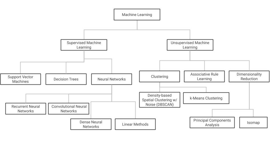
Figure 1-1. A breakdown of different types of machine learning, with a few examples of each.

Conversely, neural networks with only an input and output layer are another subset of ML known as linear models. Linear models represent the patterns they’ve learned from data using a linear function. Decision trees are another type of machine learning model that use your data to create a subset of paths with various branches. These branches approximate the results of different outcomes from your data. Finally, clustering models look for similarities between different subsets of your data and use these identified patterns to group the data into clusters.

Machine learning models, regardless of how they are depicted visually, actually comprise of mathematical functions and can therefore be implemented from scratch using a numerical software package. However, ML engineers in industry tend to employ one of several open source frameworks designed to provide intuitive APIs for building models. The majority of our examples will use TensorFlow, an open source machine learning framework created by Google with a focus on deep learning models. Within the TensorFlow library, we’ll be using the Keras API in our examples, which can be imported through tensorflow.keras. Keras is a higher-level API for building neural networks. While Keras supports many backends, we’ll be using its TensorFlow backend. In some examples we’ll be using Scikit-learn and PyTorch, which are other popular open source frameworks that provide utilities for preparing your data, along with APIs for building linear and deep models. Machine learning continues to get democratized, and one exciting development is the availability of machine learning models that can be expressed in SQL. We’ll use BigQuery ML as an example of this, especially in situations where we want to combine data preprocessing and model creation.

Machine learning problems (see Figure 1-1) can be broken into two types: supervised and unsupervised learning. Supervised learning defines problems where you know the ground truth label for your data in advance. For example, this could include labeling an image as “cat” or labeling a baby as being 2.3 kg at birth. You feed this labeled data to your model in hopes that it can learn enough to label new examples. With unsupervised learning, you do not know the labels for your data in advance, and the goal is to build a model that can find natural groupings of your data (called clustering), compress the information content (dimensionality reduction) or find association rules. The majority of this book will focus on supervised learning because the vast majority of machine learning models used in industry in production are supervised.

With supervised learning, problems can typically be defined as either classification or regression. Classification models assign your input data a label (or labels) from a discrete, predefined set of categories. Examples of classification problems include determining the type of pet breed in an image, tagging a document, or predicting whether or not a transaction is fraudulent. Regression models assign continuous, numerical values to your inputs. Examples of regression models include predicting the duration of a bike trip, a company’s future revenue, or the price of a product.

Data and Feature Engineering

Data is at the heart of any machine learning problem. When we talk about datasets, we’re referring to the data used for training, validating, and testing a machine learning model. The bulk of your data will be training data: the data fed to your model during the training process. Validation data is data that is held out from your training set and used to evaluate how the model is performing after each training epoch (or pass through the training data). The performance of the model on the validation data is used to decide when to stop the training run, and to choose hyperparameters of the machine learning model. Test data is data that is not used in the training process at all. Test data is used to evaluate how the trained model performs. Reports of performance of the machine learning model have to be stated on the independent test data. The splitting of the data has to be such that all three datasets have similar statistical properties.

The data you use to train your model can take many forms depending on the type of model you’re building. We define structured data as numerical and categorical data. Numerical data includes integer and float values, and categorical data includes data that can be divided into a finite set of groups, like type of car or education level. You can also think of this as data you would commonly find in a spreadsheet. We may also use the term tabular data to refer to structured data – the two are interchangeable. Unstructured data, on the other hand, includes data that cannot be represented as neatly. This typically includes free-form text, images, video, and audio.

Numeric data can often be fed directly to a machine learning model, where other data requires various data preprocessing before it’s ready to be sent to a model. This preprocessing step typically includes scaling numerical values, or converting non-numerical data into a numerical format that can be understood by your model. Another term for preprocessing is feature engineering. We’ll use these two terms interchangeably throughout the book.

There are various terms used to describe data as it goes through the feature engineering process. Input describes a single column in your dataset before it has been processed, and feature describes a single column after it has been processed. For example, a timestamp could be your input, and the feature would be day of the week. To get the data from timestamp to day of week, you’ll need to do some data preprocessing. This preprocessing step can also be referred to as data transformation.

An instance is the thing about which you wish to make a prediction. Given a set of features about the instance, the model will calculate a predicted value. In order to do that, the model is trained on training examples, which associate an instance with a label. A training example refers to a single instance (row) of data from your dataset that will be fed to your model. Building on the timestamp use case, a full training example might include: “day of week,” “city,” and “type of car.” A label is the output column in your dataset – the item your model is predicting. Label can refer both to the target column in your dataset (also called ground truth label) and the output given by your model (also called prediction). A sample label for the training example outlined above could be “trip duration,” in this case a float value denoting minutes.

Once you’ve assembled your dataset and determined the features for your model, data validation is the process of computing statistics on your data, understanding your schema, and evaluating the dataset to identify problems like drift and training-serving skew. Evaluating various statistics on your data can help you ensure the dataset contains a balanced representation of each feature. In cases where it’s not possible to collect more data, understanding data balance will help you design your model to account for this. Understanding your schema involves defining the data type for each feature and identifying training examples where certain values may be incorrect or missing. Finally, data validation can identify inconsistencies that may affect the quality of your training and test sets. For example, maybe the majority of your training dataset contains weekday examples while your test set contains primarily weekend examples.

The Machine Learning Process

The first step in a typical machine learning workflow is training - the process of passing training data to a model so that it can learn to identify patterns in data. After training, the next step in the process is testing how your model performs on data outside of your training dataset. This is known as model evaluation. You might run training and evaluation multiple times, performing additional feature engineering and tweaking your model architecture. Once you are happy with your model’s performance during evaluation, you’ll likely want to serve your model so that others can access it to make predictions. We use the term serving to refer to accepting incoming requests and sending back predictions by deploying the model as a microservice. The serving infrastructure could be in the cloud, on-premises, or on-device.

The process of sending new data to your model and making use of its output is called prediction. It can refer both to generating predictions from local models that have not yet been deployed, along with getting predictions from deployed models. For deployed models, we’ll refer both to online and batch prediction. Online prediction is used when you want to get predictions on a few examples in near real-time. With online prediction, the emphasis is on low latency. Batch prediction, on the other hand, refers to generating predictions on a large set of data offline. Batch prediction jobs take longer than online prediction, and are useful for precomputing predictions (such as in recommendation systems) and in analyzing your model’s predictions across a large sample of new data.

The word prediction is apt when it comes to forecasting future values, such as in predicting the duration of a bicycle ride or predicting whether a shopping cart will be abandoned. It is less intuitive in the case of image and text classification models. If an ML model looks at a text review and outputs that the sentiment is positive, it’s not really a “prediction” (there is no future outcome). Hence, you will also see word inference being used to refer to predictions. The statistical term inference is being repurposed here, but it’s not really about reasoning.

Often, the process of collecting training data, feature engineering, training, and evaluating your model are handled separately from the production pipeline. When this is the case, you’ll reevaluate your solution whenever you decide you have enough additional data to train a new version of your model. In other situations, you may have new data being ingested continuously and need to process this data immediately before sending it to your model for training or prediction. This is known as streaming. To handle streaming data, you’ll need a multi-step solution for performing feature engineering, training, evaluation, and predictions. Such multi-step solutions are called ML Pipelines.

Data and Model Tooling

There are various Google Cloud products we’ll be referencing that provide tooling for solving data and machine learning problems. These products are merely one option for implementing the design patterns referenced in this book, and not meant to be an exhaustive list. All of the products included here are serverless, allowing us to focus more on implementing machine learning design patterns rather than the infrastructure behind them.

BigQuery is an enterprise data warehouse, designed for analyzing large datasets quickly with SQL. We’ll use BigQuery in our examples for data collection and feature engineering. Data in BigQuery is organized by Datasets, and a Dataset can have multiple Tables. Many of our examples will use data from Google Cloud Public Datasets, a set of free, publicly available data hosted in BigQuery. BigQuery Public Datasets consists of hundreds of different datasets, including NOAA weather data since 1929, Stack Overflow questions and answers, open source code from GitHub, natality data, and more. To build some of the models in our examples, we’ll be using BigQuery Machine Learning (or BigQuery ML). BigQuery ML is a tool for building models from data stored in BigQuery. With BigQuery ML, we can train, evaluate, and generate predictions on our models using SQL. It supports classification and regression models, along with unsupervised clustering models. It’s also possible to import previously trained TensorFlow models to BigQuery ML for prediction.

Cloud AI Platform includes a variety of products for training and serving custom machine learning models on Google Cloud. In our examples, we’ll be using AI Platform Training and AI Platform Prediction. AI Platform Training provides infrastructure for training machine learning models on Google Cloud. With AI Platform Prediction, you can deploy your trained models and generate predictions on them using an API. Both services support TensorFlow, Scikit-Learn, and XGBoost models, along with custom containers for models built with other frameworks. We’ll also reference Explainable AI, a tool for interpreting the results of your model’s predictions, available for TensorFlow models deployed to AI Platform Prediction.

Roles

Within an organization there are many different job roles relating to data and machine learning. Below we’ll define a few common ones referenced frequently throughout the book. This book is targeted primarily at data scientists, data engineers, and ML engineers, so let’s start with those.

A data scientist is someone focused on collecting, interpreting, and processing datasets. They run statistical and exploratory analysis on data. As it relates to machine learning, a data scientist may work on data collection, feature engineering, model building, and more. Data scientists often work in Python or R in a notebook environment, and are usually the first to build out an organization’s machine learning models.

A data engineer is focused on the infrastructure and workflows powering an organization’s data. They might help manage how a company ingests data, data pipelines, and how data is stored and transferred. Data engineers implement infrastructure and pipelines around data.

Machine Learning engineers do similar tasks to data engineers, but for ML models. They take models developed by data scientists, and manage the infrastructure and operations around training and deploying those models. ML engineers help build production systems to handle updating models, model versioning, and serving predictions to end users.

The smaller the data science team at a company and the more agile the team is, the more likely it is that the same person plays multiple roles. If you are in such a situation, it is very likely that you read the above three descriptions and see yourself partially in all three categories. You might commonly start out a machine learning project as a data engineer and build data pipelines to operationalize the ingest of data. Then, you transition to the data scientist role and build the ML model(s). Finally, you put on the ML engineer hat and move the model to production. In larger organizations, machine learning projects may move through the same phases, but different teams might be involved in each phase.

There are other job roles that are related to data and machine learning, but which are not a focus audience for this book.

Research scientists focus primarily on finding and developing new algorithms to advance the discipline of ML. This could include a variety of sub-fields within machine learning, like model architectures, natural language processing, computer vision, hyperparameter tuning, model interpretability, and more. Unlike the other roles discussed here, research scientists spend most of their time prototyping and evaluating new approaches to ML, rather than building out production ML systems.

Data analysts evaluate and gather insights from data, and then summarize these insights for other teams within their organization. They tend to work in SQL, spreadsheets, and use business intelligence tools to create data visualizations to share their findings. Data analysts work closely with product teams to understand how their insights can help address business problems and create value. While data analysts focus on identifying trends in existing data and deriving insights from it, data scientists are concerned with using that data to generate future predictions and in automating or scaling out the generation of insights.

Developers are in charge of building production systems that enable end users to access ML models. They are often involved in designing the APIs that query models and return predictions in a user-friendly format via a web or mobile application. This could involve models hosted in the cloud, or models served on-device. Developers utilize the model serving infrastructure implemented by ML Engineers to build applications and user interfaces for surfacing predictions to model users.

Figure 1-2 illustrates how these different roles work together throughout an organization’s machine learning model development process.

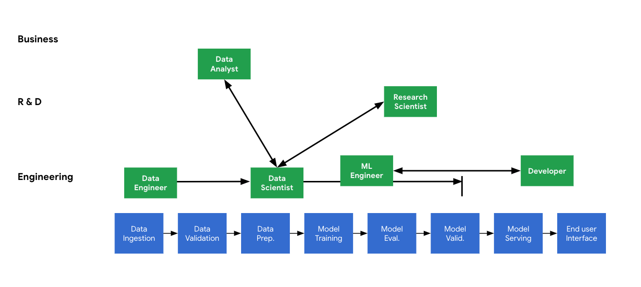
Figure 1-2. : There are many different job roles relating to data and machine learning, and these roles collaborate on the ML workflow, from data ingestion to model serving and the end user interface. For example, the data engineer works on data ingestion and data validation and collaborates closely with data scientists.

Data Quality

Machine learning models are only as reliable as the data used to train them. If you train a machine learning model on an incomplete dataset, on data with poorly selected features, or on data that doesn’t accurately represent the population using the model, your model’s predictions will be a direct reflection of that data. As a result, machine learning models are often referred to as “garbage in, garbage out.” Here we’ll highlight four important components of data quality: accuracy, completeness, consistency, and timeliness.

Data accuracy refers to both your training data’s features and the ground truth labels corresponding with those features. Understanding where your data came from and any potential errors in the data collection process can help ensure feature accuracy. After your data has been collected, it’s important to do a thorough analysis to screen for typos, duplicate entries, measurement inconsistencies in tabular data, missing features, and any other errors that may affect data quality. Duplicates in your training dataset, for example, can cause your model to incorrectly assign more weight to these data points.

Accurate data labels are just as important as feature accuracy. Your model relies solely on the ground truth labels in your training data to update its weights and minimize loss. As a result, incorrectly labeled training examples can cause misleading model accuracy. For example, let’s say you’re building a sentiment analysis model and 25% of your “positive” training examples have been incorrectly labeled as “negative.” Your model will have an inaccurate picture of what should be considered negative sentiment, and this will be directly reflected in its predictions.

To understand data completeness, let’s say you’re training a model to identify cat breeds. You train the model on an extensive dataset of cat images, and the resulting model is able to classify images into one of ten possible categories (“Bengal,” “Siamese,” and so forth) with 99% accuracy. When you deploy your model to production, however, you find that in addition to uploading cat photos for classification, many of your users are uploading photos of dogs and are disappointed with the model’s results. Because the model was trained only to identify ten different cat breeds, this is all it knows how to do. These ten breed categories are, essentially, the model’s entire “world view.” No matter what you send the model, you can expect it to slot it into one of these 10 categories. It may even do so with high confidence for an image that looks nothing like a cat. Additionally, there’s no way your model will be able to return “not a cat” if this data and label weren’t included in the training dataset.

Another aspect of data completeness is ensuring your training data contains a varied representation of each label. In the cat breed detection example, if all of your images are close-ups of a cat’s face, your model won’t be able to correctly identify an image of a cat from the side, or a full body cat image. To look at a tabular data example, if you are building a model to predict the price of real estate in a specific city but only include training examples of houses larger than 2,000 square feet, your resulting model will perform poorly on smaller houses.

The third aspect of data quality is data consistency. For large datasets, it’s common to divide the work of data collection and labeling amongst a group of people. Developing a set of standards for this process can help ensure consistency across your dataset, since each person involved in this will inevitably bring their own biases to the process. Like data completeness, data inconsistencies can be found in both data features and labels. For an example of inconsistent features, let’s say you’re collecting atmospheric data from temperature sensors. If each sensor has been calibrated to different standards, this will result in inaccurate and unreliable model predictions. Inconsistencies can also refer to data format. If you’re capturing location data, some people may write out a full street address as “Main Street” and others may abbreviate it as “Main St.” Measurement units, like miles and kilometers, can also differ around the world.

In regards to labeling inconsistencies, let’s return to the text sentiment example. In this case it’s likely people will not always agree on what is considered positive and negative when labeling training data. To solve this, you can have multiple people labeling each example in your dataset, and then take the most commonly applied label for each item. Being aware of potential labeler bias, and implementing systems to account for it, will ensure label consistency throughout your dataset.

Timeliness in data refers to the latency between when an event occurred and when it was added to your database. If you’re collecting data on application logs, for example, an error log might take a few hours to show up in your log database. For a dataset recording credit card transactions, it might take 1 day from when the transaction occurred before it is reported in your system. To deal with timeliness, it’s useful to record as much information as possible about a particular data point, and make sure that information is reflected when you transform your data into features for a machine learning model. More specifically, you can keep track of the timestamp of when an event occurred and when it was added to your dataset. Then, when performing feature engineering, you can account for these differences accordingly.

Reproducibility

In traditional programming, the output of a program is reproducible and guaranteed. For example, if you write a Python program that reverses a string, you know that an input of the word “banana” will always return an output of “ananab”. Similarly, if there’s a bug in your program causing it to incorrectly reverse strings containing numbers, you could send the program to a colleague and expect them to be able to reproduce the error with the same inputs you used (unless the bug has something to do with the program maintaining some incorrect internal state, differences in architecture such as floating point precision, or differences in execution such as threading).

Machine learning models, on the other hand, have an inherent element of randomness. When training, ML model weights are initialized with random values. These weights then converge during training as the model iterates and learns from the data. Because of this, the same model code given the same training data will produce slightly different results across training runs. This introduces a challenge of reproducibility. If you train a model to 98.1% accuracy, a repeated training run is not guaranteed to reach the same result. This can make it difficult to run comparisons across experiments.

To address this problem of repeatability, it’s common to set the random seed value used by your model to ensure that the same randomness will be applied each time you run training. In TensorFlow, you can do this by running tf.random.set_seed(value) at the beginning of your program.

Additionally, in Scikit-learn, many utility functions for shuffling your data also allow you to set a random seed value:

from sklearn.utils import shuffle
data = shuffle(data, random_state=value)

Keep in mind that you’ll need to use the same data and the same random seed when training your model to ensure repeatable, reproducible results across different experiments.

Training an ML model involves several artifacts that need to be fixed in order to ensure reproducibility: the data used, the splitting mechanism used to generate datasets used for training and validation, data preparation and model hyperparameters, and things like the batch size and learning rate schedule.

The challenge of reproducibility also applies to machine learning framework dependencies. In addition to manually setting a random seed, frameworks also implement elements of randomness internally that are executed when you call a function to train your model. If this underlying implementation changes between different framework versions, repeatability is not guaranteed. As a concrete example, if one version of a framework’s train() method makes 13 calls to rand(), and a newer version of the same framework makes 14 calls, using different versions between experiments will cause slightly different results, even with the same data and model code. Running ML workloads in containers and standardizing library versions can help ensure repeatability.

Data Drift

While machine learning models typically represent a static relationship between inputs and outputs, data can change significantly over time. Data drift refers to the challenge of ensuring your machine learning models stay relevant, and that model predictions are an accurate reflection of the environment in which they’re being used.

For example, let’s say you’re training a model to classify news article headlines into categories like “politics,” “business,” and “technology.” If you train and evaluate your model on historical news articles from the 20th century, it likely won’t perform as well on current data. Today, we know that an article with the word “smartphone” in the headline is probably about technology. However, a model trained on historical data would have no knowledge of this word. To solve for drift, it’s important to continually update your training dataset, retrain your model, and modify the weight your model assigns to particular groups of input data.

To see a less obvious example of drift, let’s look at the NOAA dataset of severe storms in BigQuery. If we were training a model to predict the likelihood of a storm in a given area, we would need to take into account the way weather reporting has changed over time. In Figure 1-3, we can see that the total number of severe storms recorded has been steadily increasing since 1950:

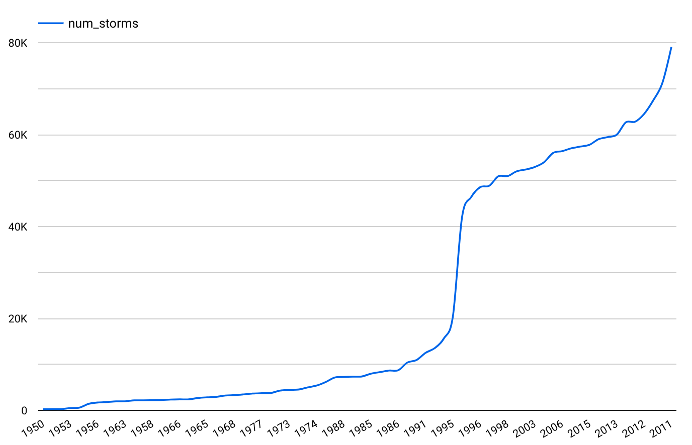
Figure 1-3. : Number of severe storms reported in a year, as recorded by NOAA from 1950 to 2011

From this trend, we can see that training a model on data before 2000 to generate predictions on storms today would lead to inaccurate predictions. In addition to the total number of reported storms increasing, it’s also important to consider other factors that may have influenced the data in Figure 1-3. For example, it’s likely that the technology for observing storms has improved over time. In the context of features, this may mean that newer data contains more information about each storm, and that a feature available in today’s data may not have been observed in 1950. Exploratory data analysis can help identify this type of drift and can inform the correct window of data to use for training.

Scale

The challenge of scaling is present throughout many stages of a typical machine learning workflow. You’ll likely encounter scaling challenges in data collection and preprocessing, training, and serving. When ingesting and preparing data for a machine learning model, the size of the dataset will dictate the tooling required for your solution. It is often the job of data engineers to build out data pipelines that can scale to handle datasets with millions of rows.

For model training, ML engineers are responsible for determining the necessary infrastructure for a specific training job. Depending on the type and size of the dataset, model training can be time consuming and computationally expensive, requiring infrastructure designed specifically for ML workloads. Image models, for instance, typically require much more training infrastructure than models trained entirely on tabular data.

In the context of model serving, the infrastructure required to support a team of data scientists getting predictions from a model prototype is entirely different from the infrastructure necessary to support a production model getting millions of prediction requests every hour. Developers and ML engineers are typically responsible for handling the scaling challenges associated with model deployment and serving prediction requests.

Multiple Objectives

Though there is often a single team responsible for building a machine learning model, many teams across an organization will make use of the model in some way. Inevitably, these teams may have different ideas of what defines a successful model.

To understand how this may play out in practice, let’s say you’re building a model to identify defective products from images. As a data scientist, your goal may be to minimize your model’s cross-entropy loss. The product manager, on the other hand, may want to reduce the number of defective products that are mis-classified and sent to customers. Finally, the executive team’s goal might be to increase revenue by 30%. Each of these goals vary in what they are optimizing for, and balancing these differing needs within an organization can present a challenge.

As a data scientist, you could translate the product team’s needs into the context of your model by saying false negatives are 5 times more costly than false positives. Therefore, you should optimize for recall over precision to satisfy this when designing your model. You can then find a balance between the product team’s goal of optimizing for precision and your goal of minimizing the model’s loss.

When defining the goals for your model, it’s important to consider the needs of different teams across an organization, and how each team’s needs relate back to the model. By analyzing what each team is optimizing for before building out your solution, you can find areas of compromise in order to optimally balance these multiple objectives.

ML Lifecycle

Building a machine learning solution is a cyclical process that begins with a clear understanding of the business goals and ultimately leads to having a machine learning model in production that benefits that goal. This high-level overview of the ML Lifecycle (see Figure 1-4) provides a useful roadmap designed to enable ML to bring value to your business. Each of the stages is equally important and failure to complete any one of these steps increases the risk in later stages of producing misleading insights or models of no value.

The ML lifecycle consists of three stages as shown in Figure 1-4: Discovery, Development, and Deployment. There is a canonical order to the individual steps of each stage, noting however that many times these steps are completed in an iterative manner and earlier steps may be revisited depending on the outcomes and insights gathered from later stages.

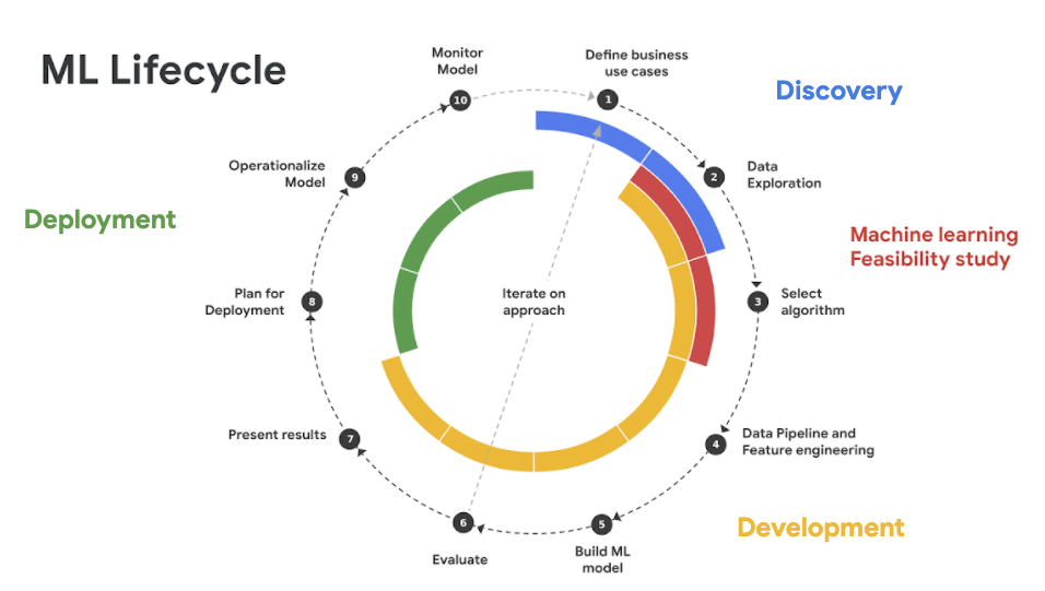
Figure 1-4. : The ML Lifecycle begins with defining the business use case and ultimately leads to having a machine learning model in production that benefits that goal.

Deployment

Assuming successful completion of the model development and evidence of promising results, the next stage is focused on productionization of the model with the first step being Planning for Deployment.

Training a machine learning model requires a substantial amount of work but to fully realize the value of that effort, the model must run in production to support the business efforts it was designed to improve. There are several approaches that achieve this goal and Deployment can look different among different organizations depending on the use case. For example, productionized ML assets could take the form of reports that can be hosted as static notebooks, or code that is wrapped in a library or package and shared for reusability, or dashboards and ML applications that can be deployed within the organization or externally via a REST API endpoint.

There are many considerations and design decisions for productionizing models. As before, many of the decisions that are made during the Discovery stage guide this step as well. How should you manage re-training the model? How to address streaming data? Should you do batch or real-time training? What about model inference? Should we plan for one-off batch inference jobs each week or do we need to support real-time prediction? Are there special throughput or latency issues to consider? Suppose our model will be used to flag fraudulent credit activity and the system will need to handle the peak rate of transactions throughout the day. Or if low latency is a priority, perhaps on-device or edge deployment is necessary. The Design Patterns addressed in Chapter 5 touch on some of the issues that arise when operationalizing an ML model.

These are important considerations and this final stage tends to be the largest hurdle for many businesses, as it can require strong coordination among different parts of the organization and integrating a variety of technical components. This difficulty is also in part due to the fact that productionization requires integrating a new process, one that relies on the machine learning model, into an existing system. This can involve dealing with legacy systems that were developed to support a single approach or there could be complex change control and production processes to navigate within the organization. Also, many times, existing systems do not have a mechanism for supporting predictions coming from a machine learning model, so new applications and workflows must be developed. It is important to anticipate these challenges and developing a comprehensive solution requires significant investment from the business operations side to make the transition as easy as possible and increase the speed-to-market.

The next step of the Deployment stage is Operationalizing the Model. This field of the practice is typically referred to as MLOps (ML Operations) and covers aspects related to automating, monitoring, testing, managing, and maintaining machine learning models in production. It is a necessary component for any company hoping to scale the number of machine learning driven applications within their organization.

One of the key characteristics of operationalized models is automated pipelines. The Development stage of the ML lifecycle is a multistep process. Building pipelines to automate these steps enables more efficient workflows and repeatable processes that improve future model development and allows for increased agility solving problems that arise. Today, open source tools like Kubeflow provide this functionality and many large software companies have developed their own end-to-end ML platforms, like Uber’s Michelangelo or Google’s TFX which is also open sourced.

Successful Operationalization incorporates components of Continuous Integration/Continuous Delivery (CI/CD) that are the familiar best practices of software development. These CI/CD practices are focused on reliability, reproducibility, speed, security and version control within code development. ML/AI workflows benefit from the same considerations though there are some notable differences. For example, in addition to the code that is used to develop the model, it is important to apply these CI/CD principles to the data including data cleaning, versioning, and orchestration of data pipelines.

The final step to be considered in the Deployment stage is Monitoring and Maintenance of the Model. Once the model has been operationalized and is in production, it’s necessary to monitor the model performance. Over time, data distributions change causing the model to become stale. This model staleness (see Figure 1-5–5) can occur for many reasons from changes in customer behavior to shifts in the environment. For this reason it is important to have in place mechanisms to efficiently monitor the machine learning model and all the various components that contribute to its performance, from data collection to the quality of the predictions during serving.

Figure 1-5. –5: Model staleness can occur for many reasons. Retraining models periodically can help to improve their performance over time.

For example, it is important to monitor the distribution of feature values to compare against the distributions that were used during the development steps. It is also important to monitor the distribution of label values to ensure that some data drift hasn’t caused an imbalance or shift in label distribution. Oftentimes, a machine learning model relies on data collected from an outside source. Perhaps your model relies on a third-party traffic API to predict wait times for car pickups or uses data from a weather API as input to a model that predicts flight delays. These APIs are not managed by your team. If that API fails or its output format changes in a significant way, then that will have consequences on your model now in production. In this case, it is important to set up monitoring to check for changes in these upstream data sources. Lastly, it is important to set up systems to monitor prediction distributions and, when possible, measure the quality of those predictions in the production environment.

Upon completion of the Monitoring step, it can be beneficial to revisit the business use case and objectively accurately assess how the machine learning model has influenced business performance. Likely, this will lead to new insights and the start of new ML projects, and the life cycle begins again.

AI Readiness

We find that different organizations working on building machine learning solutions are at different stages of AI Readiness. According to a white paper published by Google Cloud, a company’s maturity in incorporating AI into the business can typically be characterized into three phases: tactical, strategic, and transformational. Machine learning tools in these three phases goes from involving primarily manual development in the tactical phase, to involving pipelines in the strategic phase, to being fully automated in the transformational phase.

Tactical phase: Manual Development

The tactical phase of AI Readiness is often seen in organizations just beginning to explore the potential for AI to deliver, with focus on short term projects. Here the AI/ML use cases tend to be more narrow, focusing more on proof of concepts or prototypes and a direct link to the business goals may not always be clear. In this stage, organizations recognize the promise of advanced analytics work but the execution is driven primarily by individual contributors or outsourced entirely to partners and access to large-scale, quality datasets within the organization can be difficult.

Figure 1-6. : Manual development of AI models. Figure adapted from Google Cloud documentation.

Typically, in this phase there is no process to scale solutions consistently, and the ML tools used (see Figure 1-6) are developed on an ad hoc basis. Data is warehoused offline or in isolated data islands and accessed manually for Data Exploration and Analysis. There are no tools in place to automate the various phases of the ML development cycle and there is little attention paid to developing repeatable processes of the workflow. This makes it difficult to share assets within members of the organization and there is no dedicated hardware for development.

The extent of MLOps is limited to a repository of trained models and there is little distinction between testing and production environments where the final model may be deployed as an API-based solution.

Strategic phase: Utilizing Pipelines

Organizations in the strategic phase have aligned AI efforts with business objectives and priorities and ML is seen as a pivotal accelerator for the business. As such there is often senior executive sponsorship and dedicated budget for ML projects which are executed by skilled teams and strategic partners. There is infrastructure in place for these teams to easily share assets and develop ML systems that leverage both ready-to-use and custom models. There is a clear distinction between development and production environments.

Teams typically already have skills in data wrangling with expertise in descriptive and predictive analytics. Data is stored in an enterprise data warehouse and there is a unified model for centralized data and ML asset management. The development of ML models occurs as an orchestrated experiment. The ML assets and source code for these pipelines is stored in a centralized source repository and easily shared among members of the organization.

The data pipelines for developing ML models are automated utilizing a fully managed, serverless data services for ingestion and processing and are either scheduled or event-driven. So too, the ML workflow for training, evaluation and batch prediction is managed by an automated pipeline so that the stages of ML lifecycle from data validation and preparation to model training and validation (see Figure 1-7) are executed by a performance monitoring trigger. These models are stored in a centralized trained models registry and able to be deployed automatically based on predetermined model validation metrics.

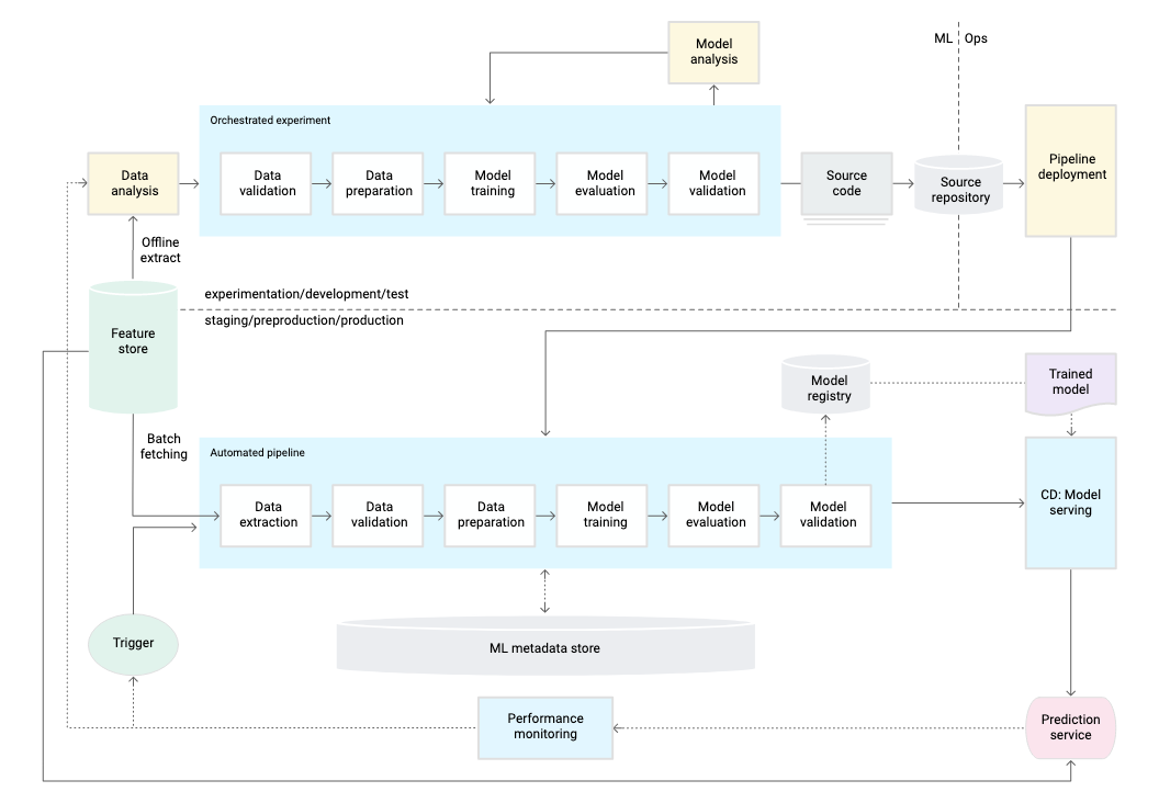
Figure 1-7. : Pipelines phase of AI development. Figure adapted from Google Cloud documentation.

There may be several ML systems deployed and maintained in production with logging, performance monitoring and notifications in place. The ML systems leverage a Model API which is capable of handling real-time data streams both for inference and to collect data which is fed into the automated ML pipeline to refresh the model for later training.

Transformational phase: Fully Automated Processes

Organizations in the transformational phase of AI Readiness are actively using AI to stimulate innovation, support agility, and cultivate a culture where experimentation and learning is ongoing. Strategic partnerships are used to innovate, co-create and augment technical resources within the company.

In this phase it is common to have product-specific AI teams embedded into the broader product teams and supported by the advanced analytics team. In this way, ML expertise is able to diffuse across various lines of business within the organization. The established common patterns and best practices as well as standard tools and libraries for accelerating ML projects are shared easily among different groups within the organization.

Datasets are stored in a platform which is accessible to all teams making it easy to discover, share and reuse datasets and ML assets. There are standardized ML feature stores and collaborations across the entire organization are encouraged. Fully automated organizations operate an integrated ML experimentation and production platform where models are built and deployed and ML practices are accessible to everyone in the organization. That platform is supported by scalable and serverless computation for batch and online data ingestion and processing. Specialized ML accelerators such as GPUs and TPUs are available on demand and there are orchestrated experiments for end-to-end data and ML pipelines.

The development and production environments are similar to the pipeline stage (see Figure 1-8) but have incorporated Continuous Integration and Continuous Delivery (CI/CD) practices into each of the various stages of their ML workflow as well. These CI/CD best practices focus on reliability, reproducibility, and version control for the code to produce the ML models as well as the data and the data pipelines and their orchestration. This allows for building, testing and packaging of various pipeline components. Model versioning is maintained by an ML Model Registry which also stores necessary ML metadata and artifacts.

Figure 1-8. : Fully automated processes support AI development. Figure adapted from Google Cloud documentation.