Chapter 3. Problem Representation Design Patterns
Chapter 2 looked at design patterns that catalog the myriad ways in which inputs to machine learning models can be represented. This chapter looks at different types of machine learning problems, and analyzes how the model architectures vary depending on the problem.
The input and the output types are two key factors impacting the model architecture. For instance, the output in supervised machine learning problems can vary depending on whether the problem being solved is a classification or regression problem. Special neural network layers exist for specific types of input data: convolutional layers for images, speech, text, and other data with spatiotemporal correlation, recurrent networks for sequential data, and so on. A huge literature has arisen around special techniques such as max pooling, attention, and so forth on these types of layers. In addition, special classes of solutions have been crafted for commonly occurring problems like recommendations (such as matrix factorization) or time-series forecasting (for example, ARIMA). Finally, a group of simpler models together with common idioms can be used to solve more complex problems -- for example, text generation often involves a classification model whose outputs are post processed using a beam search algorithm.
To limit our discussion and stay away from areas of active research, we will ignore patterns and idioms associated with specialized machine learning domains. Instead, we will focus on regression and classification and examine patterns with problem representation in just these two types of ML models.
The Reframing design pattern takes a solution that is intuitively a regression problem and poses it as a classification problem (and vice versa). The Multilabel design pattern handles the case that training examples can belong to more than one class. The Cascade design pattern addresses situations where a machine learning problem can be profitably broken into a series (or cascade) of ML problems. The Ensemble design pattern solves a problem by training multiple models and aggregating their responses. The Neutral Class design pattern looks at how to handle situations where experts disagree. The Rebalancing design pattern recommends approaches to handle highly skewed or imbalanced data.
Design Pattern 5: Reframing
The Reframing design pattern refers to changing the representation of the output of a machine learning problem. For example, we could take something that is intuitively a regression problem and instead pose it as a classification problem (and vice versa).
Problem
The first step of building any machine learning solution is framing the problem: is this a supervised learning problem? Or unsupervised? What are the features? If it is a supervised problem, what are the labels? What amount of error is acceptable? Of course, the answers to these questions must be considered in context with the training data, the task at hand, and the metrics for success.
For example, suppose we wanted to build a machine learning model to predict future rainfall amount in a given location. Starting broadly, would this be a regression or classification task? Well, since we’re trying to predict rainfall amount (for example, 0.3 cm) it makes sense to consider this as a time-series forecasting problem: given the current and historical climate and weather patterns, what amount of rainfall should we expect in a given area in the next 15 minutes? Alternately, because the label (the amount of rainfall) is a real number, we could build a regression model. As we start to develop and train our model, we find (perhaps not surprisingly) that weather prediction is harder than it sounds. Our predicted rainfall amounts are all off because, for the same set of features, it sometimes rains 0.3 cm and other times it rains 0.5 cm. What should we do to improve our predictions? Should we add more layers to our network? Or engineer more features? Perhaps more data will help? Maybe we need a different loss function?
Any of these adjustments could improve our model. But wait. Is regression the only way we can pose this task? Perhaps we can reframe our machine learning objective in a way that improves our task performance.
Solution
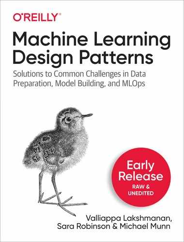
Instead of trying to predict the amount of rainfall as a regression task, we can reframe our objective as a classification problem. There are different ways this can be accomplished. One approach is to model a discrete probability distribution, as shown in Figure 3-1. Instead of predicting rainfall as a real-valued output, we model the output as a multi-class classification giving the probability that the rainfall in the next 15 minutes is within a certain range of rainfall amounts.
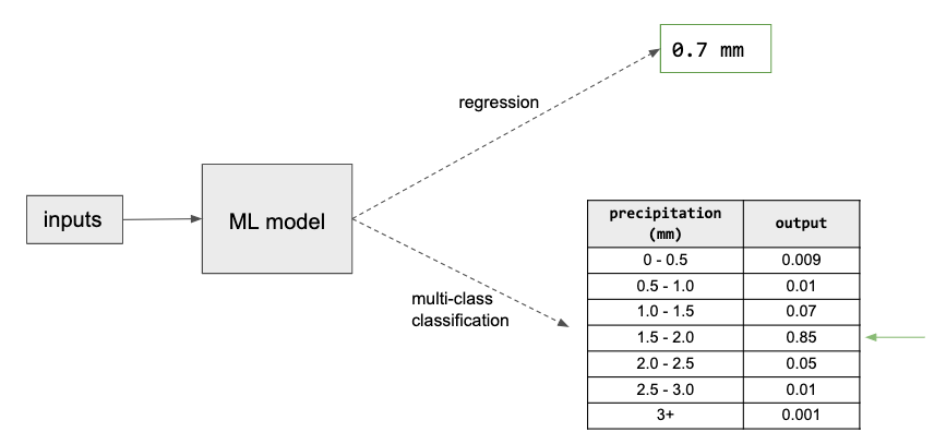
Figure 3-1. Instead of predicting precipitation as a regression output, we can instead model discrete probability distribution using a multi-class classification.
Both approaches give a prediction of the rainfall for the next 15 minutes. However, the classification approach allows the model to capture the probability distribution of rainfall of different quantities instead of having to choose the mean of the distribution. Modeling a distribution in this way is advantageous since precipitation does not exhibit the typical bell-shaped curve of a normal distribution and instead follows a Tweedie distribution which allows for a collection of points at zero, as shown in this paper. Indeed, that’s the approach taken in this paper which predicts precipitation rates in a given location using a 512-way categorical distribution. Other reasons that modeling a distribution can be advantageous is when the distribution is bimodal, or even when it is normal but with a large variance. A recent paper that beats all benchmarks at predicting protein folding structure also predicts the distance between amino acids as a 64-ways classification problem where the distances are bucketized into 64 bins.
Another reason to reframe a problem is when the objective is better in the other type of model. For example, suppose we are trying to build a recommendation system for videos. A natural way to frame this problem is as a classification problem of predicting whether a user is likely to watch a certain video. This framing, however, can lead to a recommendation system that prioritizes click-bait. It might be better to reframe this into a regression problem of predicting the fraction of the video that will be watched.
Why It Works
Changing the context and reframing the task of a problem can help when building a machine learning solution. Instead of learning a single real number, we relax our prediction target to be instead a discrete probability distribution. We lose a little precision due to bucketing, but gain the expressiveness of a full p.d.f. The discretized predictions provided by the classification model are more adept at learning a complex target than the more rigid regression model.
An added advantage of this classification framing is that we obtain posterior probability distribution of our predicted values, which provides more nuanced information. For example, suppose the learned distribution is bi-modal. By modeling a classification as a discrete probability distribution, the model is able to capture the bi-modal structure of the predictions, as Figure 3-2 illustrates. Whereas, if only predicting a single numeric value, this information would be lost. Depending on the use case, this could make the task easier to learn and substantially more advantageous.
Figure 3-2. Reframing a classification task to model a probability distribution allows the predictions to capture bimodal output. The prediction is not limited to single value as in a regression.
Capturing uncertainty
Let’s look again at the natality dataset and the task of predicting baby weight. Since baby weight is a positive real value, this is intuitively a regression problem. However, notice that for a given set of inputs, the weight_pounds (the label) can take many different values. We see that the distribution of babies’ weights for a specific set of input values (male babies born to 25-year-old mothers at 38 weeks) approximately follows a normal distribution centered at about 7.5 pounds. The code to produce the graph in Figure 3-3 can be found in the repository for this book.
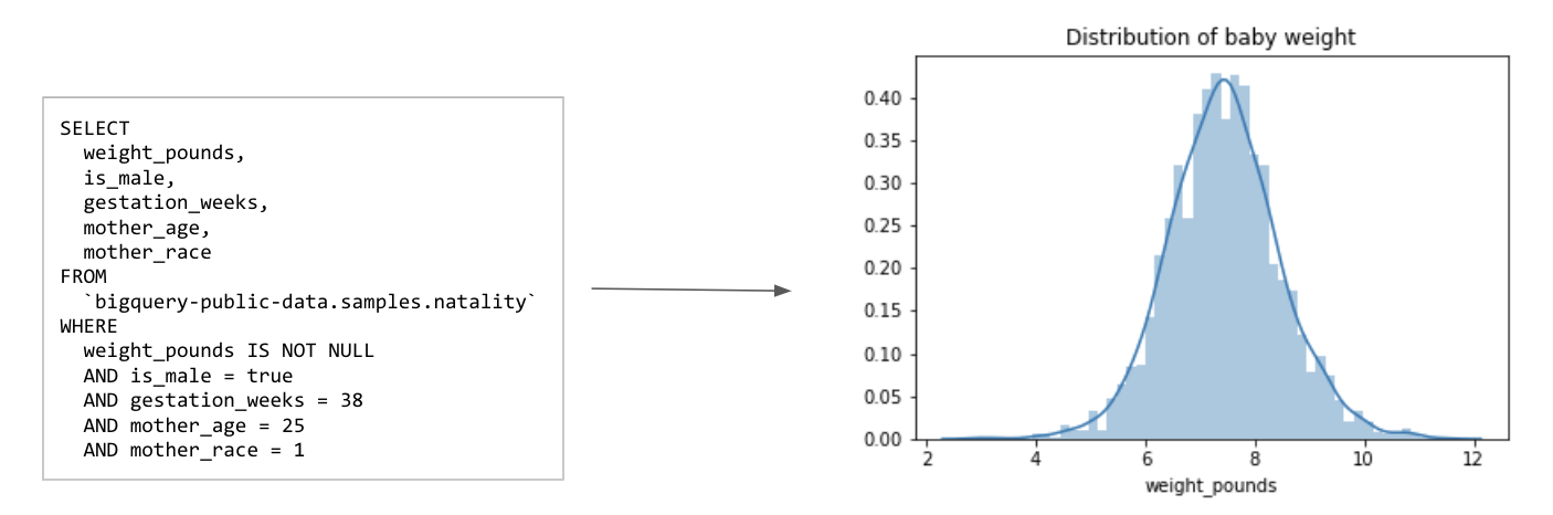
Figure 3-3. Given a specific set of inputs (for example, male babies born to 25-year-old mothers at 38 weeks) takes a range of values, approximately following a normal distribution centered at 7.5 lbs.
However, notice the width of the distribution – even though the distribution peaks at 7.5 pounds, there is a non-trivial likelihood (actually 33%) that a given baby is less than 6.5 pounds or more than 8.5 pounds! The width of this distribution indicates the irreducible error inherent to the problem of predicting baby weight. Indeed, the best root mean square error we can obtain on this problem, if we frame it as a regression problem, is the standard deviation of the distribution seen in Figure 3-3!
If we frame this as a regression problem, we’d have to state the prediction result as 7.5 +/- 1.0 (or whatever the standard deviation is). Yet, the width of the distribution will vary for different combinations of inputs, and so learning the width is another machine learning problem in and of itself. For example, at the 36th week, for mothers of the same age, the standard deviation is 1.16 pounds. Quantiles regression tries to do exactly this, but in a non-parametric way.
By reframing the problem, we train the model as a multi-class classification which learns a discrete probability distribution for the given training examples. These discretized predictions are more flexible in terms of capturing uncertainty and better able to approximate the complex target than a regression model. Of course, care has to be taken here – classification models can be hugely uncalibrated (such as the model being overly confident and wrong). At inference time, the model then predicts a collection of probabilities corresponding to these potential outputs. That is, we obtain a discrete probability density function giving the relative likelihood of any specific weight.
Note
TIP: Had the distribution been multimodal (with multiple peaks), the case for reframing the problem as a classification would be even stronger. However, it is helpful to realize that because of the law of large numbers, as long as you capture all of the relevant inputs, many of the distributions you will encounter on large datasets will be bell-shaped, although other distributions are possible. The wider the bell curve, and the more this width varies at different values of inputs, the more important it is to capture uncertainty and the stronger the case for reframing the regression problem as a classification one.
Changing the objective
In some scenarios, reframing a classification task as a regression could be beneficial. For example, suppose we had a large movie database with customer ratings on a scale from 1 to 5, for all movies that the user had watched and rated. Our task is to build a machine learning model which will be used to serve recommendations to our users.
Viewed as a classification task, we could consider building a model that takes as input a user_id, along with that user’s previous video watches and ratings, and predicts which movie from our database to recommend next. However, it is possible to reframe this problem as a regression. Instead of the model having a categorical output corresponding to a movie in our database, our model could instead carry out multi-task learning, with the model learning a number of key characteristics (such as income, customer segment, and so on) of users who are likely to watch a given movie.
Reframed as a regression task, the model now predicts the user-space representation for a given movie. To serve recommendations, we choose the set of movies that are closest to the known characteristics of a user. In this way, instead of the model providing the probability that a user will like a movie as in a classification, we would get a cluster of movies that have been watched by users like this user.
By reframing the classification problem of recommending movies to be a regression of user characteristics, we gain the ability to easily adapt our recommendation model to recommend trending videos, or classic movies, or documentaries without having to train a separate classification model each time.
This type of model approach is also useful when the numerical representation has an intuitive interpretation; for example, a latitude and longitude pair can be used instead of urban area predictions. Suppose we wanted to predict which city will experience the next viral outbreak or which New York neighborhood will have a real estate pricing surge. It could be easier to predict the latitude and longitude and choose the city or neighborhood closest to that location, rather than predicting the city or neighborhood itself.
Tradeoffs and Alternatives
There is rarely just one way to frame a problem, and it is helpful to be aware of any trade-offs or alternatives of a given implementation. For example, bucketizing the output values of a regression is an approach to reframing the problem as a classification task. Another approach is multi-task learning that combines both tasks (classification and regression) into a single model using multiple prediction heads. With any reframing technique being aware of data limitations or the risk of introducing label bias is important.
Bucketized outputs
An approach to reframing a regression task as a classification is by bucketizing the output values. For example, if our model is to be used to indicate when a baby might need critical care upon birth, the categories in Table 3-1 could be sufficient.
| High birthweight | More than 8.8 lbs |
| Average birthweight | Between 5.5 lbs and 8.8 lbs |
| Low birthweight | Between 3.31 lbs and 5.5 lbs |
| Very low birthweight | Less than 3.31 lbs |
Table 3-1. Bucketized Outputs for Babyweight
Our regression model now becomes a multi-class classification. Intuitively, it is easier to predict one out of four possible categorical cases than to predict a single value from the continuum of real numbers. Just as it would be easier to predict a binary 0 vs 1 target for is_underweight instead of four separate categories high_weight vs avg_weight vs low_weight vs very_low_weight. By using categorical outputs, our model is penalized less for getting close to the actual output value since we’ve essentially changed the output label to a range of values instead of a single real number.
In the notebook accompanying this section we train both a regression and a multi-class classification model. The regression model achieves an RMSE of 1.3 on the validation set while the classification model has an accuracy of 67%. Accurately comparing these two models is difficult since one evaluation metric is RMSE and the other is accuracy. In the end, the design decision is governed by the use case. If medical decisions are based on bucketed values, then our model should be a classification using those buckets. However, if a more precise prediction of baby weight is needed, then it makes sense to use the regression model.
Other ways of capturing uncertainty
There are other ways to capture uncertainty in regression. A simple approach is to carry out quantile regression. For example, instead of predicting just the mean, we can estimate the conditional 10th, 20th, 30th, …, 90th percentile of what needs to be predicted. Quantile regression is an extension of linear regression. Reframing, on the other hand, can work with more complex machine learning models.
Another, more sophisticated approach, is to use a framework like TensorFlow Probability to carry out regression. However, we have to explicitly model the distribution of the output. For example, if the output is expected to be normally distributed around a mean that’s dependent on the inputs, the model’s output layer would be:
tfp.layers.DistributionLambda(lambda t: tfd.Normal(loc=t, scale=1))
On the other hand, if we know the variance increases with the mean, we might be able to model it using the lambda function. Reframing, on the other hand, doesn’t require us to model the posterior distribution.
Note
TIP: When training any machine learning model, the data is key. More complex relationships typically require more training data examples to find those elusive patterns. With that in mind, it is important to consider how data requirements compare for regression or classification models. A common rule of thumb for classification tasks is that you should have 10 times the number of model features for each label category. While, for a regression model, the rule of thumb is 50 times the number of model features. Of course, these numbers are just rough heuristics and not precise. However, the intuition is that regression tasks typically require more training examples. Furthermore, this need for massive data only increases with the complexity of the task. Thus, there could be data limitations which should be considered when considering the type of model used or, in the case of classification, the number of label categories.
Precision of predictions
When thinking of reframing a regression model as a multi-class classification, the width of the bins for the output label governs the precision of the classification model. In the case of our baby weight example, if we needed more precise information from the discrete probability density function, we would need to increase the number of bins of our categorical model. Figure 3-4 shows how the discrete probability distributions would look as either a 4-way or 10-way classification.
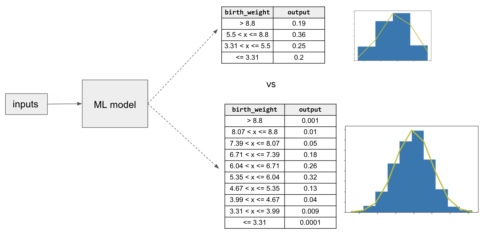
Figure 3-4. The precision of the multi-class classification is controlled by the width of the bins for the label.
The sharpness of the probability density function indicates the precision of the task as a regression. A more sharp p.d.f indicates a smaller standard deviation of the output distribution while a more wide p.d.f. indicate a larger standard deviation and thus more variance. For a very sharp density function, it would be better to stick with a regression model, as shown in Figure 3-5.

Figure 3-5. The precision of the regression is indicated by the sharpness of the probability density function for a fixed set of input values.
Restricting the prediction range
Another reason to reframe the problem is when it is essential to restrict the range of the prediction output. Let’s say, for example, that realistic output values for a regression problem are in the range [3, 20]. If we train a regression model where the output layer is a linear activation function, there is always the possibility that the model predictions will fall outside this range. One way to limit the range of the output is to reframe the problem.
Make the activation function of the last-but-one layer a sigmoid function (which is typically associated with classification) so that it is in the range [0,1] and have the last layer scale these values to the desired range:
MIN_Y =  3
MAX_Y = 20
input_size = 10
inputs = keras.layers.Input(shape=(input_size,))
h1 = keras.layers.Dense(20, 'relu')(inputs)
h2 = keras.layers.Dense(1, 'sigmoid')(h1)  # 0-1 range
output = keras.layers.Lambda(
             lambda y : (y*(MAX_Y-MIN_Y) + MIN_Y))(h2) # scaled
model = keras.Model(inputs, output)
We can verify (see the notebook on GitHub for full code) that this model now emits numbers in the range [3, 20]. Note that because the output is a sigmoid, the model will never actually hit the minimum and maximum of the range, and only get quite close to it. When we trained the model above on some random data, we got values in the range [3.03, 19.99].
Label bias
Warning
Be careful when changing the label and training task of your machine learning model, as it can inadvertently introduce label bias into your solution. Consider again the example of video recommendation we discussed in the Why It Works section.
Recommendation systems like matrix factorization can be reframed in the context of neural networks, both as a regression or classification. One advantage to this change of context is that a neural network framed as a regression or classification model can incorporate many more additional features outside of just the user and item embeddings learned in matrix factorization. So it can be an appealing alternative.
However, it is important to consider the nature of your target label when reframing the problem. For example, suppose we reframed our recommendation model to a classification task which predicts the likelihood a user will click on a certain video thumbnail. This seems like a reasonable reframing since our goal is to provide content a user will select and watch. But be careful. This change of label is not actually in line with our prediction task. By optimizing for user clicks, our model will inadvertently promote click-bait and not actually recommend content of use to the user.
Instead, a more advantageous label would be video watch time, reframing our recommendation as a regression instead. Or perhaps we can modify the classification objective to predict the likelihood that a user will watch at least half the video clip. There is often more than one suitable approach and it is important to consider the problem holistically when framing a solution.
Multi-task Learning
One alternative to reframing is multi-task learning. Instead of trying to choose between regression or classification, do both! Generally speaking, multi-task learning refers to any machine learning model in which more than one loss function is optimized. This can be accomplished in many different ways but the two most common forms of multi-task learning in neural networks is through hard parameter sharing and soft parameter sharing.
Parameter sharing refers to the parameters of the neural network being shared between the different output tasks, such as regression and classification. Hard parameter sharing occurs when the hidden layers of the model are shared between all the output tasks. In soft parameter sharing, each label has its own neural network with its own parameters and the parameters of the different models are encouraged to be similar through some form of regularization. Figure 3-6 shows the typical architecture for hard parameter sharing and short parameter sharing.

Figure 3-6. Two common implementations of multi-task learning are through hard parameter sharing and soft parameter sharing.
In the context here, we could have two heads to our model, one to predict a regression output and another to predict classification output. For example, this paper trains a computer vision model using a classification output of softmax probabilities together with a regression output to predict bounding boxes. They show this approach achieves better performance than related work that trains networks separately for the classification and localization tasks. The idea is that through parameter sharing the tasks are learned simultaneously and the gradient updates from the two loss functions inform both outputs, similar to transfer learning.
Design Pattern 6: Multilabel
The Multilabel design pattern refers to problems where we can assign more than one label to a given training example. For neural networks, this design requires changing the activation function used in the final output layer of your model, and choosing how your application will parse model output. Note that this is different from multiclass classification problems, where a single example is assigned exactly one label from a group of many (> 1) possible classes. You may also hear the Multilabel design pattern referred to as multilabel, multiclass classification since it involves choosing more than one label from a group of more than one possible class. For this pattern we’ll focus primarily on neural networks.
Problem
Often, model prediction tasks involve applying a single classification to a given training example. This prediction is determined from N possible classes where N is greater than 1. In this case, it’s common to use softmax as the activation function for the output layer. Using softmax, the output of your model is an N-element array, where the sum of all the values adds up to 1. Each value indicates the probability that a particular training example is associated with the class at that index.
For example, if your model is classifying images as either cats, dogs, or rabbits, the softmax output might look like this for a given image: [.89, .02, .09]. This means your model is predicting an 89% chance the image is a cat, 2% chance it’s a dog, and 9% chance it’s a rabbit. Because each image can have only 1 possible label in this scenario, you can take the argmax (index of the highest probability) to determine your model’s predicted class. The less common scenario is when each training example can be assigned more than one label, which is what this pattern addresses.
The Multilabel design pattern exists for models trained on all data modalities. For image classification, in the earlier cat, dog, rabbit example, we could instead use training images that each depicted multiple animals, and could therefore have multiple labels. For text models, we can imagine a few scenarios where text can be labeled with multiple tags. Using the dataset of Stack Overflow questions on BigQuery as an example, we could build a model to predict the tags associated with a particular question. As an example, the question “How do I plot a Pandas DataFrame?” could be tagged as “Python,” “Pandas,” and “visualization.” Another multilabel text classification example is a model that identifies toxic comments. For this model, you might want to flag comments with multiple toxicity labels. A comment could therefore be labeled both “hateful” and “obscene.”
This design pattern can also apply to tabular datasets. Imagine a healthcare dataset with various physical characteristics for each patient, like height, weight, age, blood pressure, and more. This data could be used to predict the presence of multiple conditions. For example, a patient could show risk of both heart disease and diabetes.
Solution
If only one label applies to a given example from our dataset, we’d use a softmax activation function in the final output layer of our model. The solution for building models that can assign more than one label to a given training example is to use the sigmoid activation function in your final output layer. Rather than generating an array where all values sum to 1 (as in softmax), each individual value in a sigmoid array is a float between 0 and 1. Building on the image example above, let’s say our training dataset included images with more than one animal. The sigmoid output for an image that contained a cat and a dog, but not a rabbit might look like the following: [.92, .85, .11]. This output means the model is 92% confident the image contains a cat, 85% confident it contains a dog, and 11% confident it contains a rabbit.
A version of this model for 28x28 pixel images with sigmoid output might look like this, using the Keras Sequential API:
model = keras.Sequential([keras.layers.Flatten(input_shape=(28, 28)),keras.layers.Dense(128, activation='relu'),keras.layers.Dense(3, activation='sigmoid')])
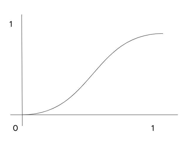
Figure 3-7. A sigmoid function.
Trade Offs
There are several special cases to consider when following the Multilabel design pattern and using sigmoid output. Next we’ll explore how to structure models that have two possible label classes, how to make sense of sigmoid results, and other important considerations for Multilabel models.
Sigmoid output for models with two classes
There are two types of models where the output can belong to two possible classes:
-
Each training example can be assigned only one class. This is also called binary classification, and is a special type of multiclass classification problem.
-
Some training examples could belong to both classes. This is a type of multilabel classification problem.
Figure 3-8–8 shows the distinction between this terminology.
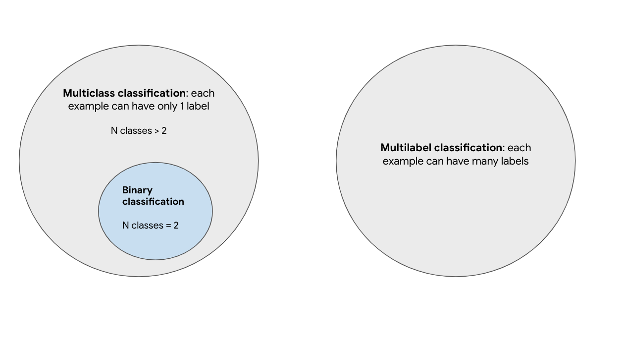
Figure 3-8. –8. Understanding the distinction between multiclass, multilabel, and binary classification problems.
The first case (binary classification) is unique in that it is the only type of multilabel classification problem where you would consider using sigmoid as your activation function. For nearly any other multiclass classification problem (for example, classifying text into 1 of 5 possible categories), you would use softmax. However, when you only have two classes, softmax is redundant. Take for example a model that predicts whether or not a specific transaction is fraudulent. If you used a softmax output in this example, here’s what a fraudulent model prediction might look like:
[.02, .98]
In this example the first index corresponds with “not fraudulent” and the second index corresponds with “fraudulent”. This is redundant because you could also represent this with a single scalar value, and thus use a sigmoid output. The same prediction could be represented as simply .98. Because each input can only be assigned a single class, you can infer from this output of .98 that the model has predicted a 98% chance of fraud and a 2% chance of non-fraud.
Therefore, for binary classification models, it is optimal to use an output shape of 1 with a sigmoid activation function. Models with a single output node are also more efficient, since they will have fewer trainable parameters and will likely train faster. Here is what the output layer of a binary classification model would look like:
keras.layers.Dense(1, activation='sigmoid')
For the second case where a training example could belong to both possible classes and fits into the Multilabel design pattern, you’ll also want to use sigmoid, this time with a 2-element output:
keras.layers.Dense(2, activation='sigmoid')
Which loss function should you use?
Now that you know when to use sigmoid as an activation function in your model, how should you choose which loss function to use with it? For the binary classification case where your model has a 1-element output, use binary cross-entropy loss. In Keras, you provide a loss function when you compile your model:
model.compile(loss='binary_crossentropy', optimizer='adam',metrics=['accuracy'])
Interestingly, you also use binary cross-entropy loss for Multilabel models with sigmoid output. You might be thinking: “Why would I use a loss function with ‘binary’ in the name for a classification task that isn’t binary?” To answer this, let’s see how binary cross-entropy loss works. Binary cross-entropy is a method for comparing two different probability distributions. By choosing a loss function that compares exactly two probability distributions, we’re looking at the difference between what our model predicted and what it should have predicted. If you break a Multilabel problem into smaller pieces, you’ll see that each label prediction in the sigmoid output is in fact its own, mini binary classification problem. For example, if you’re classifying Stack Overflow questions, determining whether a question should be tagged “Pandas” is a separate problem from determining whether it should be tagged “Matplotlib.” Consequently, if your Multilabel model predicts the tag of “Pandas” with high probability, that doesn’t preclude it from also predicting “Matplotlib” with high probability.
Returning to the image classification example where an image could contain any combination of cats, dogs, and rabbits, we can see in Figure 3-9 that this Multilabel problem is essentially three smaller binary classification problems.

Figure 3-9. Understanding the Multilabel pattern by breaking down the problem into smaller binary classification tasks.
Parsing sigmoid results
To extract the predicted label for a model with softmax output, you can simply take the argmax (highest value index) of the output array to get the predicted class. Parsing sigmoid outputs is less straightforward. Instead of taking the class with the highest predicted probability, you need to evaluate the probability of each class in your output layer and consider the probability threshold for your use case. Both of these choices are largely dependent on the end user application of your model.
Note
By threshold, we’re referring to the probability you’re comfortable with for confirming an input belongs to a particular class. For example, if you’re building a model to classify different types of animals in images, you might be comfortable saying an image has a cat even if the model is only 80% confident the image contains a cat. Alternatively, if you’re building a model that’s making healthcare predictions, you’ll likely want the model to be closer to 99% confident before confirming a specific medical condition is present or not. While thresholding is something you’ll need to consider for any type of classification model, it’s especially relevant to the Multilabel design pattern since you’ll need to determine thresholds for each class and they may be different.
To look at a specific example, let’s take the Stack Overflow dataset in BigQuery and use it to build a model that predicts the tags associated with a Stack Overflow question given its title. We’ll limit our dataset to questions that contain only five tags to keep things simple:
SELECTtitle,REPLACE(tags, "|", ",") as tagsFROM`bigquery-public-data.stackoverflow.posts_questions`WHEREREGEXP_CONTAINS(tags,r"(?:keras|tensorflow|matplotlib|pandas|scikit-learn)")
The output layer of our model would look like the following (full code for this section is available in the GitHub repo):
keras.layers.Dense(5, activation='sigmoid')
Let’s take the Stack Overflow question “What is the definition of a non-trainable parameter?” as an input example. Assuming our output indices correspond with the order of tags in our query, an output for that question might look like this:
[.95, .83, .02, .08, .65]
Our model is 95% confident this question should be tagged Keras, and 83% confident it should be tagged TensorFlow. When evaluating model predictions, we’ll need to iterate over every element in the output array and determine how we want to display those results to our end users. If 80% is our threshold for all tags, we’d show keras and tensorflow associated with this question. Alternatively, maybe we want to encourage users to add as many tags as possible and we want to show options for any tag with prediction confidence above 50%.
For examples like this one, where the goal is primarily to suggest possible tags with less emphasis on getting the tag exactly right, a typical rule of thumb is to use n_specific_tag / n_total_examples as a threshold for each class. Here, n_specific_tag is the number of examples with one tag in the dataset (for example, “Pandas”), and n_total_examples is the total number of examples in the training set across all tags. This ensures that the model is doing better than guessing a certain label based on its occurrence in the training dataset.
Note
TIP: For a more precise approach to thresholding, consider using S-Cut or optimizing for your model’s F-measure. Details on both can be found in this paper. Calibrating the per-label probabilities is often helpful as well, especially when there are thousands of labels and you want to consider the top K of them (this is common in search and ranking problems).
As you’ve seen, multilabel models provide more flexibility in how you parse predictions and require you to think carefully about the output for each class.
Dataset considerations
When dealing with single label classification tasks, you can ensure your dataset is balanced by aiming for a relatively equal number of training examples for each class. Building a balanced dataset is more nuanced for the Multilabel design pattern.
Taking the Stack Overflow dataset example, there will likely be many questions tagged as both tensorflow and keras. But there will also be questions about keras that have nothing to do with tensorflow. Similarly, we might see questions about plotting data that are tagged with both matplotlib and pandas, and questions about data pre-processing that are tagged both pandas and scikit-learn. In order for our model to learn what is unique to each tag, we’ll want to ensure the training dataset consists of varied combinations of each tag. If the majority of matplotlib questions in our dataset are also tagged pandas, the model won’t learn to classify matplotlib on its own. To account for this, think about the different relationships between labels that might be present in your model and count the number of training examples that belong to each overlapping combination of labels.
When thinking about relationships between labels in your dataset, you may also encounter hierarchical labels. ImageNet, the popular image classification dataset, contains thousands of labeled images and is often used as a starting point for transfer learning on image models. All of the labels used in ImageNet are hierarchical, meaning all images have at least one label, and many images have more specific labels that are part of a hierarchy. Here’s an example of one label hierarchy in ImageNet:
animal → invertebrate → arthropod → arachnid → spider
Depending on the size and nature of your dataset, here are two common approaches for handling hierarchical labels:
-
Use a flat approach and put every label in the same output array regardless of hierarchy, making sure you have enough examples of each “leaf node” label.
-
Use the Cascade design pattern: Build one model to identify higher level labels. Based on the high level classification, send the example to a separate model for a more specific classification task. For example, we might have an initial model that labels images as “Plant,” “Animal,” or “Person.” Depending on which labels the first model applies, we’ll send the image to different model(s) to apply more granular labels like “succulent” or “barbary lion.”
The flat approach is more straightforward than following the Cascade design pattern since it only requires one model. However, this might cause the model to lose information about more detailed label classes since there will naturally be more training examples with the higher level labels in your dataset.
Inputs with overlapping labels
The Multilabel design pattern is also useful in cases where input data occasionally has overlapping labels. Let’s take an image model that’s classifying clothing items for a catalog as an example. If you have multiple people labeling each image in the training dataset, one labeler may label an image of a skirt as “maxi skirt,” while another identifies it as “pleated skirt.” Both are correct. However, if you build a multi-class classification model on this data, passing it multiple examples of the same image with different labels, you’ll likely encounter situations where your model labels similar images differently when making predictions. Ideally you want a model that labels this image as both “maxi skirt” and “pleated skirt” as seen in Figure 3-10 below, rather than sometimes predicting only one of these labels.
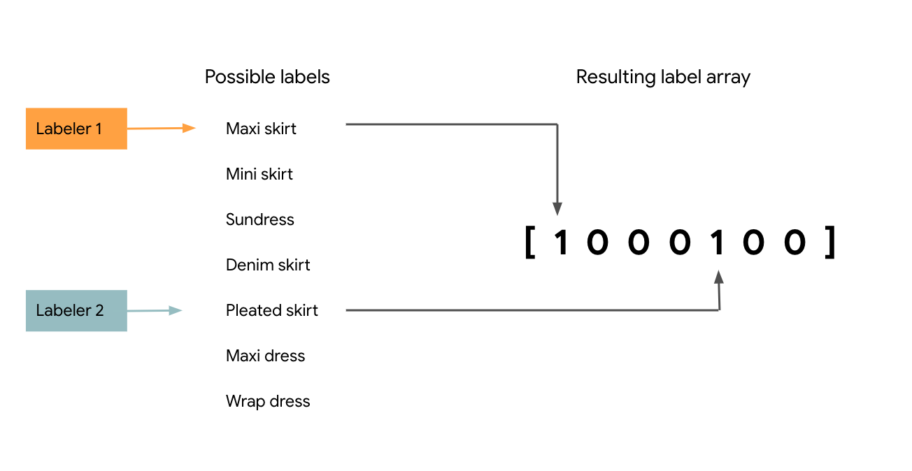
Figure 3-10. Using input from multiple labelers to create overlapping labels in cases where multiple descriptions of an item are correct.
The Multilabel design pattern solves this by allowing you to associate both overlapping labels with an image. In cases with overlapping labels where you have multiple labelers evaluating each image in your training dataset, you can choose the maximum number of labels you’d like labelers to assign to a given image, and then take the most commonly chosen tags to associate with an image during training. The threshold for “most commonly chosen tags” will depend on your prediction task and the number of human labelers you have. For example, if you have 5 labelers evaluating every image and 20 possible tags for each image, you might encourage labelers to give each image 3 tags. From this list of 15 label “votes” per image, you could then choose the 2–3 with the most votes from your labelers. When evaluating this model, take note of the average prediction confidence your model returns for each label and use this to iteratively improve your dataset and label quality.
One versus rest
Another technique for handling Multilabel classification is to train multiple binary classifiers instead of one multilabel model. This approach is called one versus rest. In the case of the Stack Overflow example where you want to tag questions as TensorFlow, Python, and Pandas, you’d train an individual classifier for each of these three tags: Python or not, TensorFlow or not, and so forth. Then you’d choose a confidence threshold and tag the original input question with tags from each binary classifier above some threshold.
The benefit of one versus rest is that you can use it with model architectures that can only do binary classification, like SVMs. It may also help with rare categories since the model will be performing only one classification task at a time on each input, and it is possible to apply the Rebalancing design pattern. The disadvantage of this approach is the added complexity of training many different classifiers, requiring you to build your application in a way that generates predictions from each of these models rather than having just one.
To summarize, use the Multilabel design pattern when your data falls into any of the following classification scenarios:
-
A single training example can be associated with mutually exclusive labels
-
A single training example can have many hierarchical labels
-
Labelers describe the same item in different ways, and each interpretation is accurate
When implementing a Multilabel model, ensure combinations of overlapping labels are well represented in your dataset, and consider the threshold values you’re willing to accept for each possible label in your model. Using a sigmoid output layer is the most common approach for building models that can handle multilabel classification. Additionally, sigmoid output can also be applied to binary classification tasks where a training example can have only one out of two possible labels.
Design Pattern 7: Ensembles
The Ensemble design pattern refers to techniques in machine learning that combine multiple machine learning models and aggregate their results to make predictions. Ensembles can be an effective means to improve performance and produce predictions that are better than any single model.
Problem
Suppose we’ve trained our baby weight prediction model, engineering special features and adding additional layers to our neural network so that the error on our training set is nearly zero. Excellent, you say! However, when we look to use our model in production at the hospital or evaluate performance on the hold out test set, our predictions are all wrong. What happened? And, more importantly, how can we fix it?
No machine learning model is perfect. To better understand where and how your model is wrong, the error of an ML model can be broken down into three parts: the irreducible error, the error due to bias and the error due to variance. The irreducible error is the inherent error in the model resulting from noise in the dataset, the framing of the problem, or bad training examples, like measurement errors or confounding factors. Just as the name implies, we can’t do much about irreducible error.
The other two, the bias and the variance, are referred to as the reducible error and here is where we can influence our model’s performance. In short, the bias is the model’s inability to learn enough about the relationship between the model’s features and labels, while the variance captures the model’s inability to generalize on new, unseen examples. A model with high bias oversimplifies the relationship and is said to be underfit. A model with high variance has learned too much about the training data and is said to be overfit. Of course, the goal of any ML model is to have low bias and low variance but, in practice, it is hard to achieve both. This is known as the bias-variance tradeoff. You can’t have your cake and eat it too. For example, increasing model complexity decreases bias but increases variance, while decreasing model complexity decreases variance but introduces more bias.
Recent work suggests that when using modern machine learning techniques such as large neural networks with high capacity, this behavior is valid only up to a point. In observed experiments, there is an “interpolation threshold” beyond which very high capacity models are able to achieve zero training error as well as low error on unseen data. Of course, you need much larger datasets in order to avoid overfitting on high capacity models.
Is there a way to mitigate this bias-variance tradeoff on small- and medium- scale problems?
Solution
Ensemble methods are meta-algorithms which combine several machine learning models as a technique to decrease the bias and/or variance and improve model performance. Generally speaking, the idea is that combining multiple models helps to improve the machine learning results. By building several models, with different inductive biases, and aggregating their outputs, we hope to get a model with better performance. In this section we’ll discuss some commonly used Ensemble methods, including bagging, boosting, and stacking.
Bagging
Bagging (short for bootstrap aggregating) is a type of parallel ensembling method and it is used to address high-variance in machine learning models. The bootstrap part of bagging refers to the datasets used for training the ensemble members. Specifically, if there are k sub-model then there are k separate datasets used for training each sub-model of the ensemble. Each dataset is constructed by randomly sampling (with replacement) from the original training dataset. This means there is a high probability that any of the k datasets will be missing some training examples, but also any dataset will likely have repeated training examples. The aggregation takes place on the output of the multiple ensemble model members, either an average in the case of a regression task or a majority vote in the case of classification.
A good example of a bagging Ensemble method is the Random Forest: multiple decision trees are trained on randomly sampled subsets of the entire training data, then the tree predictions are aggregated to produce a prediction, as shown in Figure 3-11.
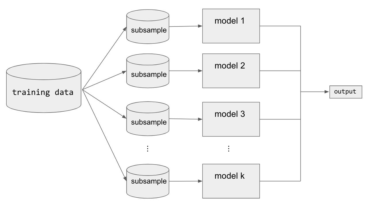
Figure 3-11. Bagging is good for decreasing variance in machine learning model output.
Popular machine learning libraries have implementations of bagging methods. For example, to implement a Random Forest regression in scikit-learn to predict baby weight from our natality dataset:
from sklearn.ensemble import RandomForestRegressor
# Create the model with 50 trees
RF_model = RandomForestRegressor(n_estimators=50,
                                 max_features='sqrt',
                                 n_jobs=-1, verbose = 1)
# Fit on training dataRF_model.fit(X_train, Y_train)
Model averaging as seen in bagging is a powerful and reliable method for reducing model variance. As we’ll see, different Ensemble methods combine multiple sub-models in different ways, sometimes using different models, different algorithms, or even different objective functions. With bagging, the model and algorithms are the same. For example, with Random Forest, the sub-models are all short Decision Trees.
Boosting
Boosting is another Ensemble technique. However, unlike bagging, boosting ultimately constructs an ensemble model with more capacity than the individual member models. For this reason, boosting provides a more effective means of reducing bias than variance. The idea behind boosting is to iteratively build an Ensemble of models where each successive model focuses on learning the examples the previous model got wrong. In short, boosting iteratively improves upon a sequence of weak learners taking a weighted average to ultimately yield a strong learner.
At the start of the boosting procedure, a simple base model f_0 is selected. For a regression task, the base model could just be the average target value; f_0 = np.mean(Y_train). For the first iteration step, the residuals delta_1 are measured and approximated via a separate model. This residual model can be anything, but typically it isn’t very sophisticated; often you’d use a weak learner like a decision tree. The approximation provided by the residual model is then added to the current prediction, and the process continues.
After many iterations the residuals tend towards zero and the prediction gets better and better at modeling the original training dataset. Notice that in Figure 3-12 the residuals for each element of the dataset decreases with each successive iteration.
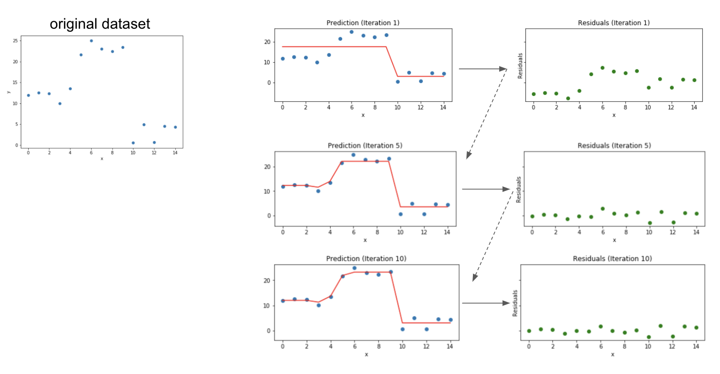
Figure 3-12. Boosting converts weak learners into strong learners by iteratively improving the model prediction.
Some of the more well-known boosting algorithms are AdaBoost, Gradient Boosting Machines and XG Boost and they have easy to use implementations in popular machine learning frameworks like scikit-learn or Tensorflow.
The implementation in scikit-learn is also straightforward:
from sklearn.ensemble import GradientBoostingRegressor
# Create the Gradient Boosting regressor
GB_model = GradientBoostingRegressor(n_estimators=1,
                                     max_depth=1,
                                     learning_rate=1,
                                     criterion='mse')
# Fit on training dataGB_model.fit(X_train, Y_train)
Stacking
Stacking is an Ensemble method which combines the outputs of a collection of models to make a prediction. The initial models, which are typically of different model types, are trained to completion on the full training dataset. Then, a secondary meta-model is trained using the initial model outputs as features. This second meta-model learns how to best combine the outcomes of the initial models to decrease the training error and can be any type of machine learning model.
To implement a Stacking Ensemble, you first train all the members of the ensemble on the training dataset. The following code calls a function fit_model which takes as arguments a model and the training dataset inputs X_train and label Y_train. This way members is a list containing all the trained models in our ensemble. The full code for this example can be found in the code repository for this book.
members = [model_1, model_2, model_3]
# fit and save models
n_members = len(members)
for i in range(n_members):
    # fit model
    model = fit_model(members[i])
    # save model
    filename = 'models/model_' + str(i + 1) + '.h5'
    model.save(filename, save_format='tf')    print('Saved {}
'.format(filename))
These sub-models are incorporated into a larger Stacking ensemble model as individual inputs. Since these input models are trained alongside the secondary ensemble model, we fix the weights of these input models. This can be done by setting layer.trainable to False for the ensemble member models:
for i in range(n_members):
    model = members[i]
    for layer in model.layers:
        # make not trainable
        layer.trainable = False
        # rename to avoid 'unique layer name' issue        layer._name = 'ensemble_' + str(i+1) + '_' + layer.name
We create the ensemble model stitching together the components using the Keras Functional API:
member_inputs = [model.input for model in members]
# concatenate merge output from each model
member_outputs = [model.output for model in members]
merge = layers.concatenate(member_outputs)
hidden = layers.Dense(10, activation='relu')(merge)
ensemble_output = layers.Dense(1, activation='relu')(hidden)
ensemble_model = Model(inputs=member_inputs, outputs=ensemble_output)
# plot graph of ensemble
tf.keras.utils.plot_model(ensemble_model, show_shapes=True, to_file='ensemble_graph.png')
# compile
ensemble_model.compile(loss='mse', optimizer='adam', metrics=['mse'])
In this example, the secondary model is a dense neural network with two hidden layers. Through training, this network learns how to best combine the results of the ensemble members when making predictions.
Why It Works
Model averaging methods like bagging work because typically the individual models that make up the ensemble model will not all make the same errors on the test set. In an ideal situation, each individual model is off by a random amount, so when their results are averaged, the random errors cancel out, and the prediction is closer to the correct answer. In short, there is wisdom in the crowd.
Boosting works well because the model is punished more and more according to the residuals at each iteration step. With each iteration, the ensemble model is encouraged to get better and better at predicting those hard to predict examples. Stacking works because it combines the best of both bagging and boosting. The secondary model can be thought of as a more sophisticated version of model averaging.
Bagging
More precisely, suppose you’ve trained k neural network regression models and average their results to create an ensemble model. If each of the models has error error_i on each example, where error_i is drawn from a zero-mean multivariate normal distribution with variance var and covariance cov, then the ensemble predictor will have error:
ensemble_error = 1./k * np.sum([error_1, error_2,...,error_k])
If the errors error_i are perfectly correlated so that cov = var, then the mean square error of the ensemble model reduces to var. In this case, model averaging doesn’t help at all. On the other extreme, if the errors error_i are perfectly un-correlated, then cov = 0 and the mean square error of the ensemble model is var/k. So, the expected square error decreases linearly with the number k of models in the ensemble1. To summarize, on average the ensemble will perform at least as well as any of the individual models in the ensemble. Furthermore, if the models in the ensemble make independent errors (for example, cov = 0) then the ensemble will perform significantly better. Ultimately, the key to success with bagging is model diversity.
This also explains why bagging is typically less effective for more stable learners like kNN, Naive Bayes, linear models or SVMs since the size of the training set is reduced through bootstrapping. Even when using the same training data neural networks can reach a variety of solutions due to random weight initializations or random mini-batch selection or different hyperparameters, creating models whose errors are partially independent. Thus, model averaging can even benefit neural networks trained on the same dataset. In fact, one recommended solution to fix the high variance of neural networks is to train multiple models and aggregate their predictions.
Boosting
The boosting algorithm works by iteratively improving the model to reduce the prediction error. Each new weak learner corrects for the mistakes of the previous prediction by modeling the residuals delta_i of each step. The final prediction is the sum of the outputs from the base learner and each of the successive weak learners as shown in Figure 3-13.

Figure 3-13. Boosting iteratively builds a strong learner from a sequence of weak learners which model the residual error of the previous iteration.
Thus, the resulting ensemble model becomes successively more and more complex, having more capacity than any one of its members. This also explains why boosting is particularly good for combatting high bias. Recall, the bias is related to the model’s tendency to be underfit. By iteratively focusing on the hard to predict examples, boosting effectively decreases the bias of the resulting model.
Stacking
Stacking can be thought of as an extension of simple model averaging where you train k models to completion on the training dataset, then average the results to determine a prediction. Simple model averaging is similar to bagging but the models in the ensemble could be of different types, while for bagging the models are of the same type. More generally, you could modify the averaging step to take a weighted average, for example, to give more weight to one model in your ensemble over the others, as shown in Figure 3-14.

Figure 3-14. The simplest form of model averaging averages the outputs of two or more different machine learning models. Alternatively, the average could be replaced with a weighted average where the weight might be based on the relative accuracy of the models.
You can think of stacking as a more advanced version of model averaging, where instead of taking an average or weighted average, you train a second machine learning model on the outputs to learn how best to combine the results to the models in your ensemble to produce a prediction as shown in Figure 3-15. This provides all the benefits of decreasing variance as with bagging techniques but also controls for high bias.

Figure 3-15. Stacking is an ensemble learning technique that combines the outputs of several different ML models as the input to a secondary ML model which makes predictions.
Tradeoffs and Alternatives
Ensemble methods have become quite popular in modern machine learning and have played a large part in winning well-known challenges, perhaps most notably the Netflix Prize. There is also a lot of theoretical evidence to back up the success demonstrated on these real-world challenges.
Increased training and design time
One downside to ensemble learning is increased training and design time. For example, for a Stacked Ensemble model, choosing the ensemble member models can require its own level of expertise and poses its own questions: Is it best to reuse the same architectures or encourage diversity? If you do use different architectures, which ones should you use? And how many? Instead of developing a single ML model (which can be a lot of work on its own!) you are now developing k models. You’ve introduced an additional amount of overhead in your model development, not to mention maintenance, inference complexity, and resource usage if the ensemble model is to go into production. This can quickly become impractical as the number of models in the ensemble increases.
Popular machine learning libraries, like scikit-learn and Tensorflow, provide easy to use implementations for many common bagging and boosting methods, like Random Forest, AdaBoost, Gradient Boosting and XGBoost. However, you should carefully consider whether the increased overhead associated with an ensemble method is worth it. Always compare accuracy and resource usage against a linear or DNN model. Note that distilling an ensemble of neural networks can often reduce complexity and improve performance.
Dropout as Bagging
Techniques like Dropout provide a powerful and effective alternative. Dropout is known as a regularization technique in deep learning but can be also understood as an approximation to bagging. Dropout in a neural network randomly (with a prescribed probability ) “turns off” neurons of the network for each mini-batch of training, essentially evaluating a bagged ensemble of exponentially many neural networks. That being said, training a neural network with dropout is not exactly the same as bagging. There are two notable differences. First, in the case of bagging the models are independent, while when training with dropout the models share parameters. Second, in bagging the models are trained to convergence on their respective training set. However, when training with dropout, the ensemble member models would only be trained for a single training step because different nodes are dropped out in each iteration of the training loop.
Decreased model interpretability
Another point to keep in mind is model interpretability. Already in deep learning, effectively explaining why your model makes the predictions it does can be difficult. This problem is compounded with Ensemble models. Consider, for example, decision trees versus the Random Forest. A decision tree ultimately learns boundary values for each feature which guide a single instance to the model’s final prediction. As such, it is easy to explain why a Decision Tree makes the predictions it did. The Random Forest, being an ensemble of many Decision Trees, loses this level of local interpretability.
Choosing the right tool for the problem
It’s also important to keep in mind the bias-variance tradeoff. Some ensemble techniques are better at addressing bias or variance than others. In particular, boosting is adapted for addressing high bias, while bagging is useful for correcting high variance. That being said, as we saw in the section on bagging, combining two models with highly correlated errors will do nothing to help lower the variance. In short, using the wrong ensemble method for your problem won’t necessarily improve performance; it will just add unnecessary overhead.
| Problem | Ensemble solution |
| High bias (underfitting) | Boosting |
| High variance (overfitting) | Bagging |
Other Ensemble methods
We’ve discussed some of the more common Ensemble techniques in machine learning. The list discussed earlier is by no means exhaustive and there are different algorithms that fit with these broad categories. There are also other Ensemble techniques, including many that incorporate a Bayesian approach or that combine neural architecture search and reinforcement learning, like Google’s AdaNet or AutoML techniques. In short, Ensemble methods are techniques which combine multiple machine learning models to improve overall model performance and can be particularly useful when addressing common training issues like high bias or high variance.
Design Pattern 8: Cascade
The Cascade design pattern addresses situations where a machine learning problem can be profitably broken into a series of ML problems. Such a cascade often requires careful design of the ML experiment.
Problem
What happens if you need to predict a value during both usual and unusual activity? The model will learn to ignore the unusual activity because it is rare. If the unusual activity is also associated with abnormal values, then trainability suffers.
For example, suppose we are trying to train a model to predict the likelihood that a customer will return an item that they have purchased. If we train a single model, the resellers’ return behavior will be lost because there are millions of retail buyers (and retail transactions) and only a few thousand resellers. We don’t really know at the time that a purchase is being made whether this is a retail buyer or a reseller. However, by monitoring other marketplaces, we have identified when items bought from us are subsequently being resold, and so our training dataset has a label that identifies a purchase as having been done by a reseller.
One way to solve this problem is to overweight the reseller instances when training the model. This is suboptimal because we need to get the more common retail buyer use case as correct as possible. We do not want to trade off a lower accuracy on the retail buyer use case for a higher accuracy on the reseller use case. However, retail buyers and resellers behave very differently; for example, while retail buyers return items within a week or so, resellers return items only if they are unable to sell it, and so the returns may be after several months. The business decision of stocking inventory is different for likely returns from retail buyers vs. resellers. Therefore, it is necessary to get both types of returns as accurate as possible. Simply overweighting the reseller instances will not work.
An intuitive way to address this problem is by using the Cascade design pattern. We break the problem into four parts:
-
Predicting whether a specific transaction is by a reseller
-
Training one model on sales to retail buyers
-
Training the second model on sales to resellers
-
In production, combining the output of the three separate models to predict return likelihood for every item purchased and the probability that the transaction is by a reseller.
This allows for the possibility of different decisions on items likely to be returned depending on the type of buyer, and ensures that both models #2 and #3 are as accurate as possible on their segment of the training data. Each of these models is relatively easy to train. The first is simply a classifier, and if the unusual activity is extremely rare, we can use the Rebalancing pattern to address it. The next two models are essentially classification models trained on different segments of the training data. The combination is deterministic, since we choose which model to run based on whether the activity belonged to a reseller.
The problem comes during prediction. At prediction time, we don’t have true labels, just the output of the first classification model. Based on the output of the first model, we will have to determine which of the two sales models we invoke. The problem is that we are training on labels, but at inference time, we will have to make decisions based on predictions. And predictions have errors. So, the second and third models will be required to make predictions on data that they might have never seen during training.
As an extreme example, assume that the address that resellers provide is always in an industrial area of the city, whereas retail buyers can live anywhere. If the first (classification) model makes a mistake and a retail buyer is wrongly identified as a reseller, the cancellation prediction model that is invoked will not have the neighborhood where the customer lives in its vocabulary.
How do we train a cascade of models where output of the one model is an input to the following model or determines the selection of subsequent models?
Solution
Any machine learning problem where the output of the one model is an input to the following model or determines the selection of subsequent models is called a Cascade. Special care has to be taken when training a Cascade of ML models.
For example, a machine learning problem that sometimes involves unusual circumstances can be solved by treating it as a Cascade of four machine learning problems:
-
A classification model to identify the circumstance
-
One model trained on unusual circumstances
-
A separate model trained on typical circumstances
-
A model to combine the output of the two separate models, because the output is a probabilistic combination of the two outputs.
This appears, at first glance, to be a specific case of the Ensemble design pattern, but is considered separately because of the special experiment design required when doing a Cascade.
As an example, assume that, in order to estimate the cost of stocking bicycles at stations, we wish to predict the distance between rental and return stations for bicycles in San Francisco. The goal of the model, in other words, is to predict the distance we need to transport the bicycle back to the rental location given features such as the time of day the rental starts, where the bicycle is being rented from, whether the renter is a subscriber or not, etc. The problem is that rentals that are longer than 4 hours involve extremely different renter behavior than shorter rentals, and the stocking algorithm requires both outputs (the probability that the rental is longer than 4 hours and the likely distance the bicycle needs to be transported). However, only a very small fraction of rentals involve such abnormal trips.
One way to solve this problem is to train a classification model to first classify trips based on whether they are Long or Typical (the full code is in the code repository of this book):
CREATE OR REPLACE MODEL mlpatterns.classify_tripsTRANSFORM(trip_type,EXTRACT (HOUR FROM start_date) AS start_hour,EXTRACT (DAYOFWEEK FROM start_date) AS day_of_week,start_station_name,subscriber_type,...)OPTIONS(model_type='logistic_reg',auto_class_weights=True,input_label_cols=['trip_type']) ASSELECTstart_date, start_station_name, subscriber_type, ...IF(duration_sec > 3600*4,'Long', 'Typical') AS trip_typeFROM `bigquery-public-data.san_francisco_bikeshare.bikeshare_trips`
It can be tempting to simply split the training dataset into two parts based on the actual duration of the rental and train the next two models, one on Long rentals and the other on Typical rentals. The problem is that the classification model just discussed will have errors. Indeed, evaluating the model on a held out portion of the San Francisco bicycle data shows that the accuracy of the model is only around 75% (see Figure 3-16). Given this, training a model on a perfect split of the data will lead to tears.

Figure 3-16. The accuracy of a classification model to predict atypical behavior is unlikely to be 100%.
Instead, after training this classification model, we need to use the predictions of this model to create the training dataset for the next set of models. For example, we could create the training dataset for the model to predict the distance of Typical rentals using:
CREATE OR REPLACE TABLE mlpatterns.Typical_tripsASSELECT* EXCEPT(predicted_trip_type_probs, predicted_trip_type)FROMML.PREDICT(MODEL mlpatterns.classify_trips,(SELECTstart_date, start_station_name, subscriber_type, ...,ST_Distance(start_station_geom, end_station_geom) AS distanceFROM `bigquery-public-data.san_francisco_bikeshare.bikeshare_trips`))WHERE predicted_trip_type = 'Typical'AND distance IS NOT NULL
Then, we should use this dataset to train the model to predict distances:
CREATE OR REPLACEMODEL mlpatterns.predict_distance_TypicalTRANSFORM(distance,EXTRACT (HOUR FROM start_date) AS start_hour,EXTRACT (DAYOFWEEK FROM start_date) AS day_of_week,start_station_name,subscriber_type,...)OPTIONS(model_type='linear_reg', input_label_cols=['distance']) ASSELECT*FROM mlpatterns.Typical_trips
Finally, our evaluation, prediction, etc. should take into account that we need to use three trained models, not just one. This is what we term the Cascade design pattern.
In practice, maintaining a Cascade workflow can become hard to keep straight. Rather than train the models individually, it is better to use a pipelines framework as shown in Figure 3-17. The key is to ensure that training datasets for the two downstream models are created each time the experiment is run based on the predictions of upstream models.

Figure 3-17. A pipeline to train the Cascade of models as a single job.
Although we introduced the Cascade pattern as a way of predicting a value during both usual and unusual activity, the Cascade pattern’s solution is capable of addressing a more general situation. The pipeline framework allows us to handle any situation where a machine learning problem can be profitably broken into a series (or cascade) of ML problems. Whenever the output of a machine learning model needs to be fed as the input to another model, the second model needs to be trained on the predictions of the first model. In all such situations, a formal pipeline experimentation framework will be helpful.
Kubeflow Pipelines provides such a framework. Because it works with containers, the underlying machine learning models and glue code can be written in nearly any programming or scripting language. Here, we will wrap the BigQuery SQL models above into Python functions using the BigQuery client library. We could use TensorFlow or scikit-learn or even R to implement individual components.
The pipeline code using Kubeflow Pipelines can be expressed quite simply as (the full code can be found in the code repository of this book):
@dsl.pipeline(name='Cascade pipeline on SF bikeshare',description='Cascade pipeline on SF bikeshare')def cascade_pipeline(project_id = PROJECT_ID):ddlop = comp.func_to_container_op(run_bigquery_ddl,packages_to_install=['google-cloud-bigquery'])c1 = train_classification_model(ddlop, PROJECT_ID)c1_model_name = c1.outputs['created_table']c2a_input =create_training_data(ddlop,PROJECT_ID, c1_model_name, 'Typical')c2b_input = create_training_data(ddlop,PROJECT_ID, c1_model_name, 'Long')c3a_model = train_distance_model(ddlop,PROJECT_ID, c2a_input.outputs['created_table'], 'Typical')c3b_model = train_distance_model(ddlop,PROJECT_ID, c2b_input.outputs['created_table'], 'Long')...
The entire pipeline can be submitted for running, and different runs of the experiment tracked using the Pipelines framework.
Use of a pipeline-experiment framework is strongly suggested whenever you will have chained ML models. Such a framework will ensure that downstream models are retrained whenever upstream models are revised and that you have a history of all the previous training runs.
Tradeoffs and Alternatives
Don’t go overboard with the Cascade design pattern -- unlike many of the design patterns we cover in this book, Cascade is not necessarily a best practice. It adds quite a bit of complexity to your machine learning workflows, and may actually result in poorer performance. Note that a pipeline-experiment framework is definitely best practice, but as much as possible, try to limit a pipeline to a single machine learning problem (ingest, preprocessing, data validation, transformation, training, evaluation, and deployment). Avoid having, as in the Cascade pattern, multiple machine learning models in the same pipeline.
Deterministic inputs
Splitting an ML problem is usually a bad idea, since an ML model can/should learn combinations of multiple factors. For example:
-
If a condition can be known deterministically from the input (holiday shopping vs. weekday shopping), we should just add the condition as one more input to the model.
-
If the condition involves an extrema in just one input (some customers who live nearby vs. far away, with the meaning of near/far needing to be learned from the data), we can use Mixed Input Representation to handle it.
The Cascade design pattern addresses an unusual scenario for which we do not have a categorical input, and for which extreme values need to be learned from multiple inputs.
Single model
The Cascade design pattern should not be used for common scenarios where a single model will suffice. For example, suppose we are trying to learn a customer’s propensity to buy. We may think we need to learn different models for people who have been comparison shopping vs. those who aren’t. We don’t really know who has been comparison shopping, but we can make an educated guess based on the number of visits, how long the item has been in the cart, and so on. This problem does not need the Cascade design pattern because it is common enough (a large fraction of customers will be comparison shopping) that the machine learning model should be able to learn it implicitly in the course of training. For common scenarios, train a single model.
Internal consistency
The Cascade is needed when you need to maintain internal consistency amongst the predictions of multiple models. Note that we are trying to do more than just predict the unusual activity. We are trying to predict returns, considering that there will be some reseller activity also. If the task is only to predict whether or not a sale is by a reseller, we’d use the Rebalancing pattern. The reason to use Cascade is that the imbalanced label output is needed as an input to subsequent models and is useful in and of itself.
Similarly, suppose that the reason we are training the model to predict a customer’s propensity to buy is to make a discounted offer. Whether or not we make the discounted offer, and the amount of discount, will very often depend on whether this customer is comparison shopping or not. Given this, we need internal consistency between the two models (the model for comparison shoppers and the model for propensity to buy). In this case, the Cascade design pattern might be needed.
Pretrained models
The Cascade is also needed when you wish to reuse the output of a pre-trained model as an input into your model. For example, let’s say you are building a model to detect authorized entrants to a building so that you can automatically open the gate. One of the inputs to your model might be the license plate of the vehicle. Instead of using the security photo directly in our model, you might find it simpler to use the output of an Optical Character Recognition (OCR) model. It is critical that you recognize that OCR systems will have errors, and so you should not train your model with perfect license plate information. Instead, you should train the model on the actual output of the OCR system. Indeed, because different OCR models will behave differently and have different errors, it is necessary to retrain the model if you change the vendor of your OCR system.
Reframing instead of Cascade
Note that in our example problem, we were trying to predict the likelihood that an item would be returned, and so this was a classification problem. Suppose instead we wish to predict hourly sales amounts. Most of the time, we will serve just retail buyers, but once in a while (perhaps 4 or 5 times a year), we will have a wholesale buyer.
This is notionally a regression problem of predicting daily sales amounts where we have a confounding factor in the form of wholesale buyers. Reframing the regression problem to be a classification problem of different sales amounts might be a better approach. Although it will involve training a classification model for each sales amount bucket, it avoids the need to get the retail vs. wholesale classification correct.
Regression in rare situations
The Cascade design pattern can be helpful when carrying out regression when some values are much more common than others. For example, you might want to predict the quantity of rainfall from a satellite image. It might be the case that on 99% of the pixels, it doesn’t rain. In such a case, it can be helpful to create a stacked classification model followed by a regression model:
-
First, predict whether or not it is going to rain.
-
For pixels where the model predicts rain is not likely, predict a rainfall amount of zero.
-
Train a regression model to predict the rainfall amount on pixels where the model predicts that rain is likely.
It is critical to realize that the classification model is not perfect, and so the regression model has to be trained on the pixels that the classification model predicts as likely to be raining (and not just on pixels that correspond to rain in the labeled dataset). For complementary solutions to this problem, also see the discussion on the Rebalancing design pattern and the Reframing design pattern.
Design Pattern 9: Neutral Class
In many classification situations, creating a Neutral class can be helpful. For example, instead of training a binary classifier that outputs the probability of an event, train a 3-class classifier that outputs disjoint probabilities for Yes, No, and Maybe. Disjoint here means that the classes do not overlap. A training pattern can belong to only one class, and so there is no overlap between Yes and Maybe, for example. The Maybe in this case is the Neutral class.
Problem
Imagine that we are trying to create a model that provides guidance on pain relievers. There are two choices: ibuprofen and acetaminophen2 and it turns out in our historical dataset that acetaminophen tends to be prescribed preferentially to patients at risk of stomach problems, and ibuprofen tends to be prescribed preferentially to patients at risk of liver damage. Beyond that, things tend to be quite random; some physicians default to acetaminophen and others to ibuprofen.
Training a binary classifier on such a dataset will lead to poor accuracy because the model will need to get the essentially arbitrary cases correct.
Solution
Imagine a different scenario. Suppose the electronic record that captures the doctors’ prescriptions also asks them whether the alternate pain medication would be acceptable. If the doctor prescribes acetaminophen, the application asks the doctor whether the patient can use ibuprofen if they already have it in their medicine cabinet.
Based on the answer to the second question, we have a Neutral class. The prescription might still be written as “acetaminophen,” but the record captures that the doctor was Neutral for this patient. Note that this fundamentally requires us to design the data collection appropriately -- we can not manufacture a Neutral class after-the-fact. We have to correctly design the machine learning problem. Correct design, in this case, starts with how we pose the problem in the first place.
If all we have is a historical dataset, we would need to get a labeling service involved. We could ask the human labelers to validate the doctors’ original choice and answer the question of whether an alternate pain medication would be acceptable.
Why It Works
We can explore the mechanism by which this works by simulating the mechanism involved with a synthetic dataset. Then, we will show that something akin to this also happens in the real-world with marginal cases.
Synthetic data
Let’s create a synthetic dataset of length N where 10 percent of the data represents patients with a history of jaundice. Since they are at risk of liver damage, their correct prescription is ibuprofen (the full code is in GitHub):
    jaundice[0:N//10] = True
    prescription[0:N//10] = 'ibuprofen'
Another 10 percent of the data will represent patients with a history of stomach ulcers; since they are at risk of stomach damage, their correct prescription is acetaminophen:
    ulcers[(9*N)//10:] = True
    prescription[(9*N)//10:] = 'acetaminophen'
The remaining patients will be arbitrarily assigned to either medication. Naturally, this random assignment will cause the overall accuracy of a model trained on just two classes to be low. In fact, we can calculate the upper bound on the accuracy. Because 80% of the training examples have random labels, the best that the model can do is to guess half of them correctly. So, the accuracy on that subset of the training examples will be 40%. The remaining 20% of the training have systematic labels, and an ideal model will learn this, so we expect that overall accuracy can be at best 60%.
Indeed training a model using scikit-learn as follows, we get an accuracy of 0.56:
    ntrain = 8*len(df)//10 # 80% of data for training
    lm = linear_model.LogisticRegression()
    lm = lm.fit(df.loc[:ntrain-1, ['jaundice', 'ulcers']],
                df[label][:ntrain])
    acc = lm.score(df.loc[ntrain:, ['jaundice', 'ulcers']],
                df[label][ntrain:])
If we create 3 classes, and put all the randomly assigned prescriptions into that class, we get, as expected, perfect (100%) accuracy. The purpose of the synthetic data was to illustrate that, provided there is random assignment at work, the Neutral Class design pattern can help us avoid losing model accuracy because of arbitrarily-labeled data.
In the real world
In real-world situations, things may not be precisely random as in the synthetic dataset, but the arbitrary assignment paradigm still holds. For example, one minute after a baby is born, the baby is assigned an “Apgar score”, a number between 1 and 10, with 10 being a baby that has come through the birthing process perfectly.
Consider a model that is trained to predict whether or not a baby will come through the birthing process healthily, or will require immediate attention (the full code is in GitHub):
CREATE OR REPLACE MODEL mlpatterns.neutral_2classes OPTIONS(model_type='logistic_reg', input_label_cols=['health']) AS SELECTIF(apgar_1min >= 9, 'Healthy', 'NeedsAttention') AS health,plurality, mother_age, gestation_weeks, ever_born FROM `bigquery-public-data.samples.natality` WHERE apgar_1min <= 10
We are thresholding the Apgar score at 9 and treating babies whose Apgar score is 9 or 10 as healthy, and babies whose Apgar score is 8 or lower as requiring attention. The accuracy of this binary classification model when trained on the natality dataset and evaluated on held-out data is 0.56.
Yet, assigning an Apgar score involves a number of relatively subjective assessments and whether a baby is assigned 8 or 9 often reduces to matters of physician preference. Such babies are neither perfectly healthy, nor do they need serious medical intervention. What if we create a Neutral class to hold these “marginal” scores? This requires creating 3 classes, with an Apgar score of 10 defined as healthy, scores of 8-9 defined as Neutral, and lower scores defined as requiring attention:
CREATE OR REPLACE MODEL mlpatterns.neutral_3classes
OPTIONS(model_type='logistic_reg', input_label_cols=['health']) AS
SELECT   IF(apgar_1min = 10, 'Healthy',
     IF(apgar_1min >= 8, 'Neutral', 'NeedsAttention')) AS health,
  plurality,
  mother_age,
  gestation_weeks,
  ever_born
FROM `bigquery-public-data.samples.natality`
WHERE apgar_1min <= 10
This model achieves an accuracy of 0.79 on a held out evaluation dataset, much higher than the 0.56 that was achieved with 2 classes.
Tradeoffs and Alternatives
The Neutral class design pattern is one to keep in mind at the beginning of a machine learning problem. Collect the right data, and you can avoid a lot of sticky problems down the line. Here are a few situations where having a Neutral class can be helpful.
When human experts disagree
The Neutral class is helpful in dealing with disagreements among human experts. Suppose we have human labelers to whom we show patient history and ask them what medication they would prescribe. We might have a clear signal for acetaminophen in some cases, a clear signal for ibuprofen in other cases, and a huge swath of cases for which human labelers disagree. The Neutral class provides a way to deal with such cases.
In the case of human labeling (unlike with the historical dataset of actual doctor actions where a patient was seen by only one doctor), every pattern is labeled by multiple experts. Therefore, we know a priori which cases humans disagree about. It might seem far simpler to simply discard such cases, and simply train a binary classifier. After all, it doesn’t matter what the model does on the Neutral cases. This has two problems:
-
False confidence tends to affect the acceptance of the model by human experts. A model that outputs a Neutral determination is often more acceptable to experts than a model that is wrongly confident in cases where the human expert would have chosen the alternative.
-
If we are training a Cascade of models, then downstream models will be extremely sensitive to the neutral classes. If we continue to improve this model, downstream models could change dramatically from version-to-version.
Another alternative is to use the agreement among human labelers as the weight of a pattern during training. Thus, if 5 experts agree on a diagnosis, the training pattern gets a weight of 1, while if the experts are split 3-2, the weight of the pattern might be only 0.6. This allows us to train a binary classifier, but overweight the classifier towards the “sure” cases. The drawback to this approach is that when the probability output by the model is 0.5, it is unclear whether it is because this reflects a situation where there was insufficient training data, or whether it is a situation where human experts disagree. Using a Neutral class to capture areas of disagreement allows us to disambiguate the two situations.
Customer satisfaction
The need for a Neutral class also arises with models that attempt to predict customer satisfaction. If the training data consists of survey responses where customers grade their experience on a scale of 1–10, it might be helpful to bucket the ratings into 3 categories: 1–4 as bad, 8–10 as good, and 5–7 is Neutral. If, instead, we attempt to train a binary classifier by thresholding at 6, the model will spend too much effort trying to get essentially neutral responses correct.
As a way to improve Embeddings
Suppose we are creating a pricing model for flights and wish to predict whether or not a customer will buy a flight at a certain price. To do this, we can look at historical transactions of flight purchases and abandoned shopping carts. However, suppose many of our transactions also include purchases by consolidators and travel agents – these are people who have contracted fares, and so the fares for them were not actually set dynamically. In other words, they don’t pay the currently displayed price.
We could throw away all the non-dynamic purchases and train the model only on customers who made the decision to buy or not buy based on the price being displayed. However, such a model will miss all the information held in the destinations that the consolidator or travel agent was interested in at various times – this will affect things like how airports and hotels are embedded. One way to retain that information while not affecting the pricing decision is to use a Neutral class for these transactions.
Reframing with Neutral class
Suppose we are training an automated trading system that makes trades based on whether it expects a security to go up or down in price. Because of stock market volatility and the speed with which new information is reflected in stock prices, trying to trade on small predicted ups and downs is likely to lead to high trading costs and poor profits over time.
In such cases, it is helpful to consider what the end-goal is. The end-goal of the ML model is not to predict whether a stock will go up or down. We will be unable to buy every stock that we predict will go up, and unable to sell stocks that we don’t hold.
The better strategy might be to buy call options3 for the ten stocks that are most likely to go up more than 5% over the next six months, and buy put options for stocks that are most likely to go down more than 5% over the next six months.
The solution, then, is to create a training dataset consisting of three classes:
-
Stocks that went up more than 5% – Call
-
Stocks that went down more than 5% – Put
-
The remaining stocks are in the Neutral category.
Rather than train a regression model on how much stocks will go up, we can now train a classification model with these three classes and pick the most confident predictions from our model.
Design Pattern 10: Rebalancing
The Rebalancing design pattern provides various approaches for handling datasets that are inherently imbalanced. By this we mean datasets where one label makes up the majority of the dataset, leaving far fewer examples of other labels.
This design pattern does not address scenarios where a dataset lacks representation for a specific population or real-world environment. Cases like this can often only be solved by additional data collection. The Rebalancing design pattern primarily addresses how to build models with datasets where few examples exist for a specific class or classes.
Problem
Machine learning models learn best when they are given a similar number of examples for each label class in a dataset. Many real world problems, however, are not so neatly balanced. Take for example a fraud detection use case, where you are building a model to identify fraudulent credit card transactions. Fraudulent transactions are much rarer than regular transactions, and as such, there is less data on fraud cases available to train a model. The same is true for other problems like detecting whether someone will default on a loan, identifying defective products, predicting the presence of a disease given medical images, filtering spam emails, flagging error logs in a software application, and more.
Imbalanced datasets apply to many types of models, including binary classification, multiclass classification, multilabel classification, and regression. In regression cases, imbalanced datasets refer to data with outlier values that are either much higher or lower than the median in your dataset.
A common pitfall in training models with imbalanced label classes is relying on misleading accuracy values for model evaluation. If you train a fraud detection model and only 5% of your dataset contains fraudulent transactions, chances are your model will train to 95% accuracy without any modifications to the dataset or underlying model architecture. While this 95% accuracy number is technically correct, there’s a good chance your model is guessing the majority class (in this case, non-fraud) for each example. As such, it’s not learning anything about how to distinguish the minority class from other examples in your dataset.
To avoid leaning too much on this misleading accuracy value, it’s worth looking at the model’s confusion matrix to see accuracy for each class. The confusion matrix for a poorly performing model trained on an imbalanced dataset often looks something like Figure 3-18.
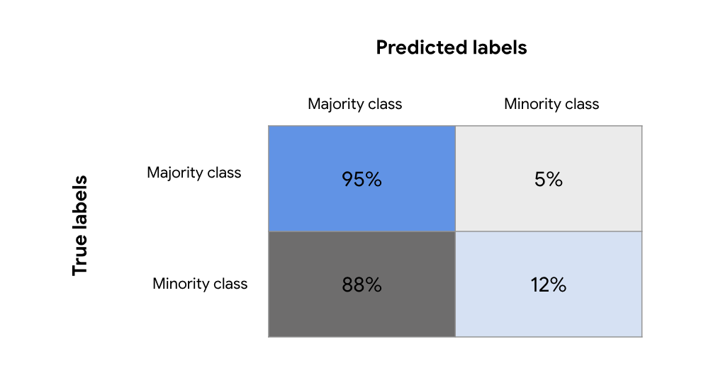
Figure 3-18. Confusion matrix for a model trained on an imbalanced dataset without dataset or model adjustments.
In this example, the model correctly guesses the majority class 95% of the time, but only guesses the minority class correctly 12% of the time. Typically, the confusion matrix for a high performing model has percentages close to 100 down the diagonal.
Solutions
First, since accuracy can be misleading on imbalanced datasets, it’s important to choose an appropriate evaluation metric when building your model. Then, there are various techniques you can employ for handling inherently imbalanced datasets at both the dataset and model level. Downsampling changes the balance of your underlying dataset, while weighting changes how your model handles certain classes. Upsampling duplicates examples from your minority class, and often involves applying augmentations to generate additional samples. We’ll also look at approaches for reframing your problem: changing it to a regression task, analyzing your model’s error values for each example, or clustering.
Choosing an evaluation metric
For imbalanced datasets like the one in our fraud detection example, it’s best to use metrics like precision, recall, or F-measure to get a complete picture of how your model is performing. Precision measures the percentage of positive classifications that were correct out of all positive predictions made by the model. Conversely, recall measures the proportion of actual positive examples that were identified correctly by the model. The biggest difference between these two metrics is the denominator used to calculate them. For precision, the denominator is the total number of positive class predictions made by your model. For recall, it is the number of actual positive class examples present in your dataset.
A perfect model would have both precision and recall of 1.0, but in practice these two measures are often at odds with each other. The F-measure is a metric that ranges from 0 to 1 and takes both precision and recall into account. It is calculated as:
2 * (precision * recall / (precision + recall))
Let’s return to the fraud detection use case to see how each of these metrics plays out in practice. For this example, let’s say our test set contains a total of 1,000 examples, 50 of which should be labeled as fraudulent transactions. For these examples, our model predicts 930 / 950 non-fraudulent examples correctly, and 15 / 50 fraudulent examples correctly. We can visualize these results in Figure 3-19:
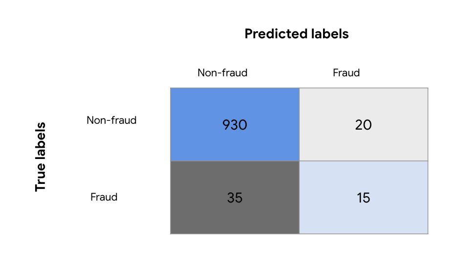
Figure 3-19. sample predictions for a fraud detection model.
In this case our model’s precision is 15 / 35 (42%), recall is 15 / 50 (30%), and F-measure is 35%. These do a much better job capturing our model’s inability to correctly identify fraudulent transactions compared to accuracy, which is 945 / 1000 or 94.5%. Therefore, for models trained on imbalanced datasets, metrics other than accuracy are preferred. In fact, accuracy may even go down when optimizing for these metrics, but that is ok since precision, recall, and F-score are a better indication of model performance in this case.
Note that, when evaluating models trained on imbalanced datasets, we need to use unsampled data when calculating success metrics. This means that no matter how you modify your dataset for training per the solutions we’ll outline below, you should leave your test set as is so it provides an accurate representation of the original dataset. In other words, your test set should have roughly the same class balance as your original dataset. For the example above, that would be 5% fraud / 95% non-fraud.
If you are looking for a metric that captures the performance of the model across all thresholds, average precision-recall is a more informative metric than Area Under the Curve (AUC) for model evaluation. This is because average precision-recall places more emphasis on how many predictions the model got right out of the total number it assigned to the positive class. This gives more weight to the positive class, which is important for imbalanced datasets. The area under the ROC curve, on the other hand, treats both classes equally and is less sensitive to model improvements, which isn’t optimal in situations with imbalanced data.
Downsampling
Downsampling is a solution for handling imbalanced datasets by changing the underlying dataset, rather than the model. With downsampling, you decrease the number of examples from the majority class used during model training. To see how this works, let’s take a look at the synthetic fraud detection dataset on Kaggle.4 Each example in the dataset contains various information about the transaction, including the transaction type, the amount of the transaction, and the account balance both before and after the transaction took place. The dataset contains 6.3 million examples, only 8,000 of which are fraudulent transactions. That’s a mere 0.1% of the entire dataset.
While a large dataset can often improve a model’s ability to identify patterns, it’s less helpful when the data is significantly imbalanced. If we train a model on this entire dataset (6.3M rows) without any modifications, chances are we’ll see a misleading accuracy of 99.9% as a result of the model randomly guessing the non-fraudulent class each time. We can solve for this by removing a large chunk of the majority class from the dataset.
We’ll take all 8k of the fraudulent examples and set them aside to use when training the model. Then, we’ll take a small, random sample of the non-fraudulent transactions. We’ll then combine with our 8k fraudulent examples, re-shuffle the data, and use this new, smaller dataset to train a model. Here’s how we could implement this with Pandas:
data = pd.read_csv('fraud_data.csv')
# Split into separate dataframes for fraud / not fraud
fraud = data[data['isFraud'] == 1]
not_fraud = data[data['isFraud'] == 0]
# Take a random sample of non fraud rows
not_fraud_sample = not_fraud.sample(random_state=2, frac=.005)
# Put it back together and shuffle
df = pd.concat([not_fraud_sample,fraud])df = shuffle(df, random_state=2)
Following this, our dataset would contain 25% fraudulent transactions, much more balanced than the original dataset with only 0.1% in the minority class. It’s worth experimenting with the exact balance used when downsampling. Here we used a 25/75 split, but different problems might require closer to a 50/50 split to achieve decent accuracy.
Downsampling is usually combined with the Ensemble pattern, following these steps:
-
Downsample the majority class and use all the instances of the minority class
-
Train a model and add to the ensemble
-
Repeat
During inference, take the median output of the ensemble models.
We discussed a classification example here, but downsampling can also be applied to regression models where you’re predicting a numerical value. In this case, taking a random sample of majority class samples will be more nuanced since the majority “class” in your data includes a range of values rather than a single label.
Weighted classes
Another approach to handling imbalanced datasets is to change the weight your model gives to examples from each class. Note that this is a different use of the term “weight” than the weights (or parameters) learned by your model during training, which you cannot set manually. By weighting classes, you tell your model to treat specific label classes with more importance during training. You’ll want your model to assign more weight to examples from the minority class. Exactly how much importance your model should give to certain examples is up to you, and is a parameter you can experiment with.
In Keras, you can pass a class_weights parameter to your model when you train it with fit(). class_weights is a dict, mapping each class to the weight Keras should assign to examples from that class. But how should you determine the exact weights for each class? The class weight values should relate to the balance of each class in your dataset. For example, if the minority class accounts for only 0.1% of the dataset, a reasonable conclusion is that our model should treat examples from that class with 1000x more weight than the majority class. In practice, it’s common to divide this weight value by 2 for each class so that the average weight of an example is 1.0. Therefore, given a dataset 0.1% of values representing the minority class, we could calculate the class weights with the following code:
num_minority_examples = 1num_majority_examples = 999total_examples = num_minority_examples + num_majority_examplesminority_class_weight = 1/(num_minority_examples/total_examples)/2majority_class_weight = 1/(num_majority_examples/total_examples)/2# Pass the weights to Keras in a dict# Thekey is the index of each classkeras_class_weights = {0: majority_class_weight, 1: minority_class_weight}
We’d then pass these weights to our model during training:
model.fit(
    train_data,
    train_labels,
    class_weight=keras_class_weights)
In BigQuery ML, you can set AUTO_CLASS_WEIGHTS = True in the OPTIONS block when creating your model to have different classes weighted based on their frequency of occurrence in the training data.
While it can be helpful to follow a heuristic of class balance for setting class weights, the business application of a model might also dictate the class weights you choose to assign. For example, let’s say we have a model classifying images of defective products. If the cost of shipping a defective product is 10 times that of incorrectly classifying a normal product, we would choose 10 as the weight for our minority class.
Upsampling
Another common technique for handling imbalanced datasets is upsampling. With upsampling, you over-represent your minority class by both replicating minority class examples and generating additional, synthetic examples. This is often done in combination with downsampling the majority class. This approach – combining downsampling and upsampling – was proposed in 2002 and referred to as Synthetic Minority Over-sampling Technique (SMOTE). SMOTE provides an algorithm that constructs these synthetic examples by analyzing the feature space of minority class examples in the dataset and then generates similar examples within this feature space using a nearest neighbors approach. Depending on how many similar data points you choose to consider at once (also referred to as the number of nearest neighbors), the SMOTE approach randomly generates a new minority class example between these points.
Let’s look at the Pima Indian Diabetes Dataset to see how this works at a high level. 34% of this dataset contains examples of patients who had diabetes, so we’ll consider this our minority class. Table 3-1 shows a subset of columns for two minority class examples:
Table 3-1. A subset of features for two training examples from the minority class (has Diabetes) in the Pima Indian Diabetes Dataset.
| Glucose | BloodPressure | SkinThickness | BMI |
| 148 | 72 | 35 | 33.6 |
| 183 | 64 | 0 | 23.3 |
A new, synthetic example based on these two actual examples from the dataset might look like Table 3-2, calculating by the midpoint between each of these column values:
Table 3-2. A synthetic example generated from the two minority training examples above using the SMOTE approach.
| Glucose | BloodPressure | SkinThickness | BMI |
| 165.5 | 68 | 17.5 | 28.4 |
The SMOTE technique refers primarily to tabular data, but similar logic can be applied to image datasets. For example, if you’re building a model to distinguish between Bengal and Siamese cats and only 10% of your dataset contains images of Bengals, you can generate additional variations of the Bengal cats in your dataset through image augmentation using the Keras ImageDataGenerator class. With a few parameters, this class will generate multiple variations of the same image by rotating, cropping, adjusting brightness, and more.
Tradeoffs and Alternatives
There are a few other alternative solutions for building models with inherently imbalanced datasets, including reframing the problem and handling cases of anomaly detection. We’ll also explore several important considerations for imbalanced datasets: overall dataset size, the optimal model architectures for different problem types, and explaining minority class prediction.
Reframing and Cascade
Reframing your problem is another approach for handling imbalanced datasets. First, you might consider switching your problem from classification to regression or vice versa utilizing the techniques described in the Reframing design pattern section and training a Cascade of models. For example, let’s say you have a regression problem where the majority of your training data falls within a certain range, with a few outliers. Assuming you care about predicting outlier values, you could convert this to a classification problem by bucketing the majority of the data in one bucket and the outliers in another.
Imagine we’re building a model to predict baby weight using the BigQuery natality dataset. Using Pandas, we can create a histogram of a sample of the baby weight data to see the weight distribution:
SELECT
  weight_pounds
FROM
  `bigquery-public-data.samples.natality`
LIMIT 10000df.plot(kind='hist')
Figure 3-20 shows the resulting histogram.
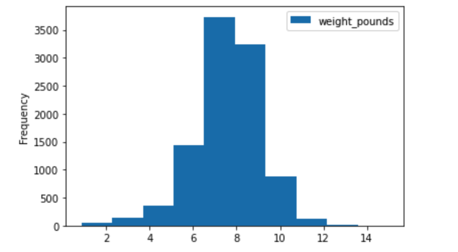
Figure 3-20. A histogram depicting the distribution of baby weight for 10,000 examples in the BigQuery natality dataset.
If we count the number of babies weighing 3 lbs in the entire dataset, there are approximately 96,000 (.06% of the data). Babies weighing 12 lbs make up only .05% of the dataset. To get good regression performance over the entire range, we can combine downsampling with the Reframing and Cascade design patterns. First, we’ll split the data into three buckets: “underweight,” “average,” and “overweight.” We can do that with the following query:
SELECT
  CASE
    WHEN weight_pounds < 5.5 THEN "underweight"
    WHEN weight_pounds > 9.5 THEN "overweight"
  ELSE
  "average"
END
  AS weight,
  COUNT(*) AS num_examples,
  round(count(*) / sum(count(*)) over(), 4) as percent_of_dataset
FROM
  `bigquery-public-data.samples.natality`
GROUP BY  1
Table 3-3 shows the results:
Table 3-3. The percentage of each weight class present in the natality dataset.
| weight | num_examples | percent_of_dataset |
| Average | 123781044 | 0.8981 |
| Underweight | 9649724 | 0.07 |
| Overweight | 4395995 | 0.0319 |
For demo purposes, we’ll take 100,000 examples from each class to train a model on an updated, balanced dataset:
SELECT
  is_male,
  gestation_weeks,
  mother_age,
  weight_pounds,
  weight
FROM (
  SELECT
    *,
    ROW_NUMBER() OVER (PARTITION BY weight ORDER BY RAND()) AS row_num
  FROM (
    SELECT
      is_male,
      gestation_weeks,
      mother_age,
      weight_pounds,
      CASE
        WHEN weight_pounds < 5.5 THEN "underweight"
        WHEN weight_pounds > 9.5 THEN "overweight"
      ELSE
      "average"
    END
      AS weight,
    FROM
      `bigquery-public-data.samples.natality`
    LIMIT
      4000000) )
WHERE  row_num < 100000
We can save the results of that query to a table, and with a more balanced dataset we can now train a classification model to label babies as “underweight,” “average,” or “overweight”:
CREATE OR REPLACE MODEL
  `project.dataset.baby_weight_classification` OPTIONS(model_type='logistic_reg',
    input_label_cols=['weight']) AS
SELECT
  is_male,
  weight_pounds,
  mother_age,
  gestation_weeks,
  weight
FROM  `project.dataset.baby_weight`
Another approach is to use the Cascade pattern, training three separate regression models for each class. Then, we can use our multi-design pattern solution by passing our initial classification model an example, and using the result of that classification to decide which regression model to send the example to for numeric prediction.
Anomaly detection
There are two approaches to handling regression models for imbalanced datasets:
-
Use the model’s error on a prediction as a signal
-
Cluster incoming data, and compare the distance of each new data point to existing clusters
To better understand each solution, let’s say we’re training a model on data collected by a sensor to predict temperature in the future. In this case we’d need the model output to be a numerical value.
For the first approach – using error as a signal – after training a model we would then compare the model’s predicted value with the actual value for the current point in time. If there was a significant difference between the predicted and actual current value, we could flag the incoming data point as an anomaly. Of course, this requires a model trained with good accuracy on enough historical data to rely on its quality for future predictions. The main caveat for this approach is that it requires you to have new data readily available, so that you can compare the incoming data with the model’s prediction. As a result, it works best for problems involving streaming or time-series data.
In the second approach – clustering data – you start by building a model with a clustering algorithm, a modeling technique that organizes your data into clusters. Clustering is an unsupervised learning method, meaning it looks for patterns in your dataset without any knowledge of ground truth labels. A common clustering algorithm is k-means, which we can implement with BigQuery ML. The following shows how to train a k-means model on the BigQuery natality dataset using three features:
CREATE OR REPLACE MODEL
  `project-name.dataset-name.baby_weight` OPTIONS(model_type='kmeans',
    num_clusters=4) AS
SELECT
  weight_pounds,
  mother_age,
  gestation_weeks
FROM
  `bigquery-public-data.samples.natality`LIMIT 10000
The resulting model will cluster our data into four groups. Once the model has been created, we can then generate predictions on new data and look at that prediction’s distance from existing clusters. If the distance is high, we can flag the data point as an anomaly. To generate a cluster prediction on our model, we can run the following query passing it a made-up average example from the dataset:
SELECT
  *
FROM
  ML.PREDICT (MODEL `project-name.dataset-name.baby_weight`,
    (
    SELECT
      7.0 as weight_pounds,
      28 as mother_age,
      40 as gestation_weeks
     )  )
The query results in Table 3-4 show us the distance between this data point and the model’s generated clusters, called centroids.
Table 3-4. The distance between our average weight example data point and each of the clusters generated by our k-means model.
| CENTROID_ID | NEAREST_CENTROIDS_DISTANCE.CENTROID_ID | NEAREST_CENTROIDS_DISTANCE.DISTANCE |
| 4 | 4 | 0.29998627812137374 |
| 1 | 1.2370167418282159 | |
| 2 | 1.376651161584178 | |
| 3 | 1.6853517159990536 |
This example clearly fits into centroid 4, as seen by the small distance (.29).
We can compare this to the results we get if we send an outlier, underweight example to the model, as shown in Table 3-5.
Table 3-5. The distance between our underweight example data point and each of the clusters generated by our k-means model.
| CENTROID_ID | NEAREST_CENTROIDS_DISTANCE.CENTROID_ID | NEAREST_CENTROIDS_DISTANCE.DISTANCE |
| 3 | 3 | 3.061985789261998 |
| 4 | 3.3124603501734966 | |
| 2 | 4.330205096751425 | |
| 1 | 4.658614918595627 |
Here, the distance between this example and each centroid is quite large. We could then use these high distance values to conclude that this data point might be an anomaly. This unsupervised clustering approach is especially useful if you don’t know the labels for your data in advance. Once you’ve generated cluster predictions on enough examples, you could then build a supervised learning model using the predicted clusters as labels.
Number of minority class examples available
While the minority class in our first fraud detection example only made up 0.1% of the data, the dataset was large enough that we still had 8,000 fraudulent data points to work with. For datasets with even fewer examples of the minority class, downsampling may make the resulting dataset too small for a model to learn from. There isn’t a hard and fast rule for determining how many examples is too few to use downsampling, since it largely depends on your problem and model architecture. A general rule of thumb is that if you only have hundreds of examples of the minority class, you might want to consider a solution other than downsampling for handling dataset imbalance.
It’s also worth noting that the natural effect of removing a subset of your majority class is losing some information stored in those examples. This might slightly decrease your model’s ability to identify the majority class, but often the benefits of downsampling still outweigh this.
Combining different techniques
The downsampling and class weight techniques described above can be combined for optimal results. To do this, start by downsampling your data until you find a balance that works for your use case. Then, based on the label ratios for the rebalanced dataset, use the method described in the weighted classes section to pass new weights to your model. Combining these approaches can be especially useful when you have an anomaly detection problem and care most about predictions for your minority class. For example, if you’re building a fraud detection model, you’re likely much more concerned about the transactions your model flags as “fraud” rather than the ones it flags as “non-fraud.” Additionally, as mentioned by SMOTE, the approach of generating synthetic examples from the minority class is often combined with removing a random sample of examples from the minority class.
Downsampling is also often combined with the Ensemble design pattern. Using this approach, instead of entirely removing a random sample of your majority class, you use different subsets of it to train multiple models and then ensemble those models. To illustrate this, let’s say we have a dataset with 100 minority class examples and 1000 majority examples. Rather than removing 900 examples from our majority class to perfectly balance the dataset, we’d randomly split the majority examples into 10 groups with 100 examples each. We’d then train 10 classifiers, each with the same 100 examples from our minority class and 100 different, randomly selected values from our majority class. The bagging technique illustrated in Figure 3-11 would work well for this approach.
In addition to combining these data-centric approaches, you can also adjust the threshold for your classifier to optimize for precision or recall depending on your use case. If you care more that your model is correct whenever it makes a positive class prediction, optimize your prediction threshold for recall. This can apply in any situation where you want to avoid false positives. Alternatively, if it is more costly to miss a potential positive classification even when you might get it wrong, optimize your model for recall.
Choosing a model architecture
Depending on your prediction task, there are different model architectures to consider when solving problems with the Rebalancing design pattern. If you’re working with tabular data and building a classification model for anomaly detection, research has shown that decision tree models perform well on these types of tasks. Tree-based models also work well on problems involving small and imbalanced datasets. XGBoost, Scitkit-learn, and TensorFlow all have methods for implementing decision tree models.
We can implement a binary classifier in XGBoost with the following code:
# Build the model
model = xgb.XGBClassifier(
    objective='binary:logistic'
)
# Train the model
model.fit(
    train_data,
    train_labels)
You can use downsampling and class weights in each of these frameworks to further optimize your model using the Rebalancing design pattern. For example, to add weighted classes to our XGBClassifier above, we’d add a scale_pos_weight parameter, calculated based on the balance of classes in our dataset.
If you’re detecting anomalies in time-series data, LSTM models work well for identifying patterns present in sequences. Clustering models are also an option for tabular data with imbalanced classes. For imbalanced datasets with image input, use deep learning architectures with downsampling, weighted classes, upsampling, or a combination of these techniques. For text data, however, generating synthetic data is less straightforward and it’s best to rely on downsampling and weighted classes.
Regardless of the data modality you’re working with, it’s useful to experiment with different model architectures to see which performs best on your imbalanced data.
Importance of explainability
When building models for flagging rare occurrences in data such as anomalies, it’s especially important to understand how your model is making predictions. This can both verify that the model is picking up on the correct signals to make its predictions, and help explain the model’s behavior to end users. There are a few tools available to help you interpret your models and explain predictions, including: the open source framework SHAP, the What-If Tool, and Explainable AI on Google Cloud.
Model explanations can take many forms, one of which is called attribution values. Attribution values tell you how much each feature in your model influenced the model’s prediction. Positive attribution values mean a particular feature pushed our model’s prediction up, and negative attribution values mean the feature pushed our model’s prediction down. The higher the absolute value of an attribution, the bigger impact it had on our model’s prediction. In image and text models, attributions can show you the pixels or words that signaled your model’s prediction most. For tabular models, attributions provide numerical values for each feature, indicating its overall effect on the model’s prediction.
After training a TensorFlow model on the synthetic fraud detection dataset from Kaggle and deploying it to Explainable AI on Google Cloud, let’s take a look at some examples of instance-level attributions. In Figure 3-21, we see two example transactions that our model correctly identified as fraud, along with their feature attributions.
Figure 3-21. Feature attributions from Explainable AI for two correctly classified fraudulent transactions.
In the first example where the model predicted a 99% chance of fraud, the old balance at the origin account before the transaction was made was the biggest indicator of fraud. In the second example, our model was 89% confident in its prediction of fraud with the amount of the transaction identified as the biggest signal of fraud. However, the balance at the origin account made our model less confident in its prediction of fraud and explains why the prediction confidence is slightly lower by ten percentage points.
Explanations are important for any type of machine learning model, but we can see how they are especially useful for models following the Rebalancing design pattern. When dealing with imbalanced data, it’s important to look beyond our model’s accuracy and error metrics to verify that it’s picking up on meaningful signals in our data.
Summary
This chapter looked at different ways to represent a prediction task through the lens of model architecture and model output. Thinking about how you’ll apply your model can guide your decision on the type of model to build, and how to format your output for prediction. With this in mind, we started with the Reframing design pattern, which explores changing your problem from a regression to classification task (or vice versa) to improve the quality of your model. You can do this by re-formatting the label column in your data. Next we explored the Multilabel design pattern, which addresses cases where an input to your model can be associated with more than one label. To handle this case, use the sigmoid activation function on your output layer with binary cross entropy loss.
Whereas the Reframing and Multilabel patterns focus on formatting model output, the Ensemble design pattern addresses model architecture and includes various methods for combining multiple models to improve upon machine learning results from a single model. Specifically, the Ensemble pattern includes bagging, boosting, and stacking – all different techniques for aggregating multiple models into one ML system. The Cascade design pattern is also a model-level approach, and involves breaking a machine learning problem into several smaller problems. Unlike Ensemble models, the Cascade pattern requires outputs from an initial model to be inputs into downstream models. Because of the complexity Cascade models can create, you should only use it when you have a scenario where the initial classification labels are disparate and equally important.
Next we looked at the Neutral Class design pattern, which addresses problem representation at the output level. This pattern improves a binary classifier by adding a third “neutral” class. This is useful in cases where you want to capture arbitrary or less polarizing classifications that don’t fall into either of the distinct binary categories. Finally, the Rebalancing design pattern provides solutions for cases where you have an inherently imbalanced dataset. This pattern proposes using downsampling, weighted classes, or specific reframing techniques to solve for datasets with imbalanced label classes.
Chapters 2 and 3 focused on the initial steps for structuring your machine learning problem, specifically formatting input data, model architecture options, and model output representation. In the next chapter, we’ll navigate the next step in the machine learning workflow – design patterns for training models.
1 c.f. For the explicit computation of these values see Chap. 7 of Deep Learning by Goodfellow et al., MIT Press, 2015.
2 This is just an example being used for illustrative purposes; please don’t take this as medical advice!
3 See https://en.wikipedia.org/wiki/Option_(finance) for a primer on call and put options.
4 Find this dataset on Kaggle: https://www.kaggle.com/ntnu-testimon/paysim1. The dataset was generated based on the PaySim research proposed in this paper: E. A. Lopez-Rojas , A. Elmir, and S. Axelsson. “PaySim: A financial mobile money simulator for fraud detection”. In: The 28th European Modeling and Simulation Symposium-EMSS, Larnaca, Cyprus. 2016