Chapter 4. Patterns That Modify Model Training
Machine learning models are usually trained iteratively, and this iterative process is informally called the training loop. In this chapter, we discuss what the typical training loop looks like, and catalog a number of situations in which you might want to do something different.
Typical Training Loop
Machine learning models can be trained using different types of optimization. Decision trees are often built node-by-node based on an information gain measure. In genetic algorithms, the model parameters are represented as genes, and the optimization method involves techniques that are based on evolutionary theory. However, the most common approach to determining the parameters of machine learning models is gradient descent.
Stochastic Gradient Descent
On large datasets, gradient descent is applied to mini batches of the input data to train everything from linear methods and neural networks to deep neural networks (DNNs) and support vector machines (SVMs). This is called Stochastic Gradient Descent (SGD), and extensions of SGD (such as Adam and Adagrad) are the de facto optimizers used in modern-day machine learning frameworks.
Because SGD requires training to take place iteratively on small batches of the training dataset, training a machine learning model happens in a loop. SGD finds a minimum, but is not a closed form solution, and so we have to detect whether the model convergence has happened. Because of this, the error (called the loss) on the training dataset has to be monitored. Overfitting can happen if the model complexity is higher than can be afforded by the size and coverage of the dataset. Unfortunately, you cannot know whether the model complexity is too high for a particular dataset until you actually train that model on that dataset. Therefore, evaluation needs to be done within the training loop, and error metrics on a withheld split of the training data, called the validation dataset, have to be monitored as well. Because the training and validation datasets have been used in the training loop, it is necessary to withhold yet another split of the training dataset, called the testing dataset, to report the actual error metrics that could be expected on new and unseen data. This evaluation is carried out at the end.
Keras Training Loop
The typical training loop in Keras looks like this:
model = keras.Model(...)
model.compile(optimizer=keras.optimizers.Adam(),
              loss=keras.losses.categorical_crossentropy(),
              metrics=['accuracy'])
history = model.fit(x_train, y_train,
                    batch_size=64,
                    epochs=3,
                    validation_data=(x_val, y_val))
results = model.evaluate(x_test, y_test, batch_size=128))
model.save(...)
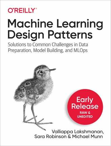
Here, the model uses the Adam optimizer to carry out stochastic gradient descent on the cross entropy over the training dataset, and reports out the final accuracy obtained on the testing dataset. The model fitting loops over the training dataset three times (each traversal over the training dataset is termed an epoch) with the model seeing batches consisting of 64 training examples at a time. At the end of every epoch, the error metrics are calculated on the validation dataset and added to the history. At the end of the fitting loop, the model is evaluated on the testing dataset, saved, and potentially deployed for serving, as shown in Figure 4-1.
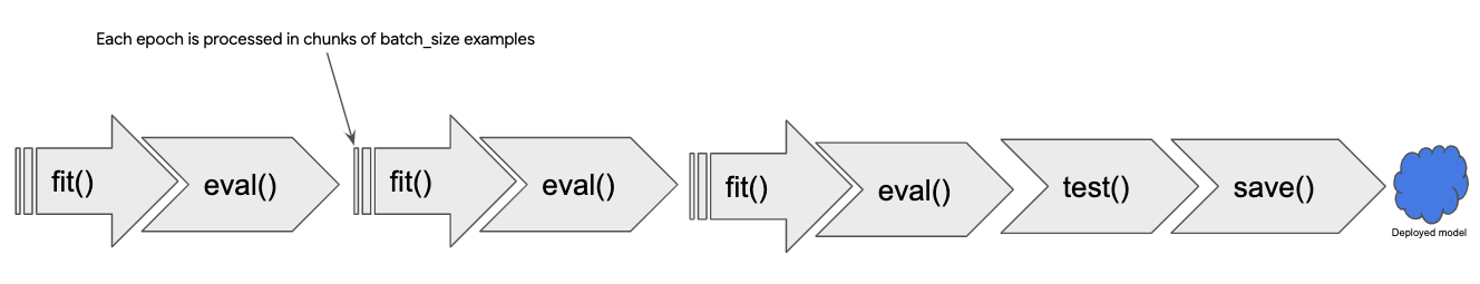
Figure 4-1. A typical training loop consisting of 3 epochs. Each epoch is processed in chunks of batch_size examples. At the end of the third epoch, the model is evaluated on the testing dataset, and saved for potential deployment as a web service.
Instead of using the prebuilt fit() function, we could also write a custom training loop that iterates over the batches explicitly, but we will not need to do this for any of the design patterns discussed in this chapter.
Training Design Patterns
The design patterns covered in this chapter all have to do with modifying the typical training loop in some way. In Useful Overfitting, we forego the use of a validation or testing dataset because we want to intentionally overfit on the training dataset. In Checkpoints, we store the full state of the model periodically, so that we have access to partially trained models. When we use checkpoints, we usually also use Virtual Epochs, wherein we decide to carry out the inner loop of the fit(), not on the full training dataset but on a fixed number of training examples. In Transfer Learning, we take part of a previously trained model, freeze the weights, and incorporate these non-trainable layers into a new model that solves the same problem, but on a smaller dataset. In Distribution Strategy, the training loop is carried out at scale over multiple workers, often with caching, hardware acceleration, and parallelization. Finally, in Hyperparameter Tuning, the training loop is itself inserted into an optimization method to find the optimal set of model hyperparameters.
Design Pattern 11: Useful Overfitting
Useful Overfitting is a design pattern where we forgo the use of generalization mechanisms because we want to intentionally overfit on the training dataset. In situations where overfitting can be beneficial, this design pattern recommends that we carry out machine learning without regularization, dropout, or a validation dataset for early stopping.
Problem
The goal of a machine learning model is to generalize and make reliable predictions on new, unseen data. If your model overfits the training data (for example, continues to decrease the training error beyond the point at which validation error starts to increase), then its ability to generalize suffers and so do your future predictions. Introductory machine learning textbooks advise avoiding overfitting by using early stopping and regularization techniques.
Consider, however, a situation of simulating the behavior of physical or dynamical systems like those found in climate science, computational biology, or computational finance. In such systems, the time dependence of observations can be described by a mathematical function or set of partial differential equations (PDEs). Although the equations that govern many of these systems can be formally expressed, they don’t have a closed-form solution. Instead, classical numerical methods have been developed to approximate solutions to these systems. Unfortunately, for many real-world applications these methods can be too slow to be used in practice.
Consider the situation shown in Figure 4-2. Observations collected from the physical environment are used as inputs (or initial starting conditions) for a physics-based model that carries out iterative, numerical calculations to calculate the precise state of the system. Suppose all the observations have a finite number of possibilities (for example, temperature will be between 60C and 80C in increments of 0.01C). It is then possible to create a training dataset for the machine learning system consisting of the complete input space and calculate the labels using the physical model.
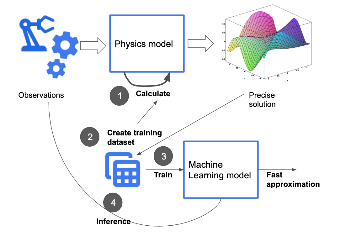
Figure 4-2. One situation when it is acceptable to overfit is when the entire domain space of observations can be tabulated, and a physical model capable of computing the precise solution is available.
The ML model needs to learn this precisely calculated and non-overlapping lookup table of inputs to outputs. Splitting such a dataset into a training dataset and an evaluation dataset is counterproductive because we would then be expecting the model to learn parts of the input space it will not have seen in the training dataset.
Solution
In this scenario, there is no “unseen” data that needs to be generalized to, since all possible inputs have been tabulated. When building a machine learning model to learn such a physics model or dynamical system, there is no such thing as overfitting. The basic machine learning training paradigm is slightly different. Here, there is some physical phenomenon that you are trying to learn which is governed by an underlying partial differential equation or system of partial differential equations. Machine learning merely provides a data-driven approach to approximate the precise solution and concepts like overfitting must be reevaluated.
For example, a ray-tracing approach is used to simulate the satellite imagery that would result from the output of numerical weather prediction models. This involves calculating how much of a solar ray gets absorbed by the predicted hydrometeors (rain, snow, hail, ice pellets, and so on) at each atmospheric level. There is a finite number of possible hydrometeor types and a finite number of heights that the numerical model predicts. So the ray-tracing model has to apply optical equations to a large, but finite set of inputs.
The equations of radiative transfer govern the complex dynamical system of how electromagnetic radiation propagates in the atmosphere and forward radiative transfer models are an effective means of inferring the future state of satellite images. However, classical numerical methods to compute the solutions to these equations can take tremendous computational effort and are too slow to use in practice.
Enter machine learning. It is possible to use machine learning to build a model that approximates solutions to the forward radiative transfer model, see Figure 4-3. This ML approximation can be made close enough to the solution of the model that was originally achieved by using more classical methods. The advantage is that inference using the learned ML approximation (which needs to just calculate a closed formula) takes only a fraction of the time required to carry out ray tracing (which would require numerical methods). At the same time, the training dataset is too large (multiple terabytes) and too unwieldy to use as a lookup table in production.
Figure 4-3. Architecture for using a neural network to model the solution of a partial differential equation to solve for I(r,t,n).
There is an important difference between training an ML model to approximate the solution to a dynamical system like this and training an ML model to predict baby weight based on natality data collected over the years. Namely, the dynamical system is a set of equations governed by the laws of electromagnetic radiation – there is no unobserved variable, no noise, and no statistical variability. For a given set of inputs, there is only one precisely calculable output. There is no overlap between different examples in the training dataset. For this reason, we can toss out concerns about generalization. We want our ML model to fit the training data as perfectly as possible, to “overfit.”
This is counter to the typical approach of training an ML model where considerations of bias, variance, and generalization error play an important role. Traditional training says that it is possible for a model to learn the training data “too well,” and that training your model so that the train loss function is equal to zero is more of a red flag than cause for celebration. Overfitting of the training dataset in this way causes the model to give misguided predictions on new, unseen data points. The difference here is that we know in advance there won’t be unseen data, thus the model is approximating a solution to a PDE over the full input spectrum. If your neural network is able to learn a set of parameters where the loss function is zero, then that parameter set determines the actual solution of the PDE in question.
Why It Works
If all possible inputs can be tabulated, then as shown by the dotted curve in Figure 4-4, an overfit model will still make the same predictions as the “true” model if all possible input points are trained for. So overfitting is not a concern. We have to take care that inferences are made on rounded off values of the inputs, with the rounding determined by the resolution with which the input space was gridded.
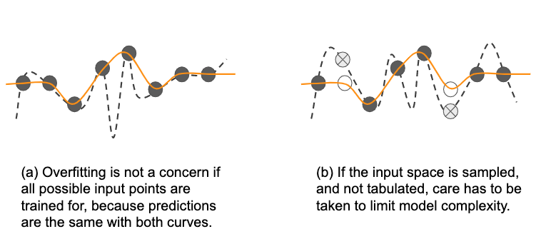
Figure 4-4. Overfitting is not a concern if all possible input points are trained for, because predictions are the same with both curves.
Is it possible to find a model function that gets arbitrarily close to the true labels? One bit of intuition as to why this works comes from the Uniform Approximation Theorem of deep learning, which, loosely put, states that any function (and its derivatives) can be approximated by a neural network with at least one hidden layer and any “squashing” activation function, like sigmoid. This means that no matter what function we are given, so long as it’s relatively well behaved, there exists a neural network with just one hidden layer that approximates that function as closely as we want.1
Deep learning approaches to solving differential equations or complex dynamical systems aim to represent a function defined implicitly by a differential equation, or system of equations, using a neural network.
Overfitting is useful when the following two conditions are met:
-
There is no noise, so the labels are accurate for all instances.
-
You have the complete dataset at your disposal (you have all the examples there are). In this case, overfitting becomes interpolating the dataset.
Tradeoffs and Alternatives
We introduced overfitting as being useful when the set of inputs can be exhaustively listed, and the accurate label for each set of inputs can be calculated. If the full input space can be tabulated, overfitting is not a concern because there is no unseen data. However, the Useful Overfitting design pattern is useful beyond this narrow use case. In many real-world situations, even if one or more of these conditions has to be relaxed, the concept that overfitting can be useful remains valid.
Interpolation and chaos theory
The machine learning model essentially functions as an approximation to a lookup table of inputs to outputs. If the lookup table is small, just use it as a lookup table! There is no need to approximate it by a machine learning model. An ML approximation is useful in situations where the lookup table will be too large to effectively use. It is when the lookup table is too unwieldy that it becomes better to treat it as the training dataset for a machine learning model that approximates the lookup table.
Note that we assumed that the observations would have a finite number of possibilities. For example, we posited that temperature would be measured in 0.01C increments and lie between 60C and 80C. This will be the case if the observations are made by digital instruments. If this is not the case, the ML model is needed to interpolate between entries in the lookup table.
Machine learning models interpolate by weighting unseen values by the distance of these unseen values from training examples. Such interpolation works only if the underlying system is not chaotic. In chaotic systems, even if the system is deterministic, small differences in initial conditions can lead to dramatically different outcomes. Nevertheless, in practice, each specific chaotic phenomenon has a specific resolution threshold beyond which it is possible for models to forecast it over short time periods. Therefore, provided the lookup table is fine-grained enough and the limits of resolvability are understood, useful approximations can result.
Monte Carlo methods
In reality, tabulating all possible inputs might not be possible, and you might take a Monte Carlo approach of sampling the input space to create the set of inputs, especially where not all possible combinations of inputs are physically possible.
In such cases, overfitting is technically possible (see Figure 4-5, where the unfilled circles are approximated by wrong estimates shown by crossed circles).

Figure 4-5. If the input space is sampled, not tabulated, then you need to take care to limit model complexity.
However, even here, you can see that the ML model will be interpolating between known answers. The calculation is always deterministic, and it is only the input points that are subject to random selection. Therefore, these known answers do not contain noise, and because there are no unobserved variables, errors at unsampled points will be strictly bounded by the model complexity. Here, the overfitting danger comes from model complexity and not from fitting to noise. Overfitting is not as much of a concern when the size of the dataset is larger than the number of free parameters. Therefore, using a combination of low-complexity models and mild regularization provides a practical way to avoid unacceptable overfitting in the case of Monte Carlo selection of the input space.
Data-driven discretizations
Although deriving a closed form solution is possible for some PDEs, determining solutions using numerical methods is more common. Numerical methods of PDEs are already a deep field of research, and there are many books, courses, and journals devoted to the subject. One common approach is to use finite difference methods, similar to Runge-Kutta methods for solving ordinary differential equations. This is typically done by discretizing the differential operator of the PDE and finding a solution to the discrete problem on a spatio-temporal grid of the original domain. However, when the dimension of the problem becomes large, this mesh-based approach fails dramatically due to the curse of dimensionality because the mesh spacing of the grid must be small enough to capture the smallest feature size of the solution. So, to achieve 10x higher resolution of an image requires 10,000x more compute power, because the mesh grid must be scaled in four dimensions accounting for space and time.
However, it is possible to use machine learning (rather than Monte Carlo methods) to select the sampling points, to create data-driven discretizations of PDEs. In the paper, "Learning data-driven discretizations for PDEs“, Bar-Sinai et al. demonstrate the effectiveness of this approach. The authors use a low-resolution grid of fixed points to approximate a solution via a piecewise polynomial interpolation using standard finite-difference methods as well as one obtained from a neural network. The solution obtained from the neural network vastly outperforms the numeric simulation in minimizing the absolute error, in some places achieving a 10^2 order of magnitude improvement. While increasing the resolution requires substantially more compute power using finite-difference methods, the neural network is able to maintain high performance only marginal additional cost. Techniques like the Deep Galerkin Method can then use deep learning to provide a mesh-free approximation of the solution to the given PDE. In this way, solving the PDE is reduced to a chained optimization problem (see the Cascade design pattern in Chapter 3).
Unbounded domains
The Monte Carlo and data-driven discretization methods both assume that sampling the entire input space, even if imperfectly, is possible. That’s why the ML model was treated as aninterpolation between known points.
Generalization and the concern of overfitting become difficult to ignore whenever we are unable to sample points in the full domain of the function -- for example, for functions with unbounded domains or projections along a time axis into the future. In these settings, it is important to consider overfitting, underfitting, and generalization error. In fact, it’s been shown that although techniques like the Deep Galerkin Method do well on regions that are well sampled, a function that is learned this way does not generalize well on regions outside the domain that were not sampled in the training phase. This can be problematic for using ML to solve PDEs that are defined on unbounded domains, since it would be impossible to capture a representative sample for training.
Overfitting a batch
In practice, training neural networks requires a lot of experimentation, and a practitioner must make many choices, from the size and architecture of the network to the choice of the learning rate, weight initializations, or other hyperparameters.
Overfitting on a small batch is a good sanity check both for the model code as well as the data input pipeline. Just because the model compiles and the code runs without errors doesn’t mean you’ve computed what you think you have or that the training objective is configured correctly. A complex enough model should be able to overfit on a small enough batch of data, assuming everything is set up correctly. So, if you’re not able to overfit a small batch with any model, it’s worth rechecking your model code, input pipeline, and loss function for any errors or simple bugs. Overfitting on a batch is a useful technique when training and troubleshooting neural networks.
You can test your Keras model code in this way using the tf.data.Dataset you’ve written for your input pipeline. For example, if your training data input pipeline is called trainds, we’ll use .batch(...) to pull a single batch of data. You can find the full code for this example in the repository accompanying this book.
BATCH_SIZE = 256
single_batch = trainds.batch(BATCH_SIZE).take(1)
Then, when training the model, instead of calling the full trainds Dataset inside the .fit method, use the single batch that we created:
model.fit(single_batch.repeat(),
          validation_data=evalds,
          …)
Note that we apply the .repeat() so that we won’t run out of data when training on that single batch. This ensures that we take the one batch over and over again while training. Everything else (the validation dataset, model code, engineered features, and so on) remains the same.
Note
TIP Rather than choose an arbitrary sample of the training dataset, we recommend that you overfit on a small dataset each of whose examples has been carefully verified to have correct labels. Design your neural network architecture such that it is able to learn this batch of data precisely and get to zero loss. Then take the same network and train it on the full training dataset.
TIP Overfitting goes beyond just a batch. From a more holistic perspective, overfitting follows the general advice commonly given with regards to deep learning and regularization. The best fitting model is a large model that has been properly regularized. In short, if your deep neural network isn’t capable of overfitting your training dataset, you should be using a bigger one. Then, once you have a large model that overfits the training set, you can apply regularization to improve the validation accuracy, even though training accuracy may decrease.
Design Pattern 12: Checkpoints
In Checkpoints, we store the full state of the model periodically, so that we have partially trained models available. These partially trained models can serve as the final model (in the case of early stopping) or as the starting points for continued training (in the cases of machine failure and fine-tuning).
Problem
The more complex a model is (for example, the more layers and nodes a neural network has), the larger the dataset that is needed to train it effectively. This is because more complex models tend to have more tunable parameters. As model sizes increase, the time it takes to fit one batch of examples also increases. As the data size increases (and assuming batch sizes are fixed), the number of batches also increases. Therefore, in terms of computational complexity, this double whammy means that training will take a long time.
At the time of writing, training an English to German translation model on a state-of-the-art Tensor Processing Unit (TPU) pod on a relatively small dataset takes about two hours. On real datasets of the sort used to train smart devices, the training can take several days.
When we have training that takes this long, the chances of machine failure are uncomfortably high. If there is a problem, we’d like to be able to resume from an intermediate point, instead of from the very beginning.
Solution
At the end of every epoch, we can save the model state. Then, if the training loop is interrupted for any reason, we can go back to the saved model state and restart. However, when doing this, we have to make sure to save the intermediate model state, not just the model. What does that mean?
Once training is complete, we save or export the model so that we can deploy it for inference. An exported model does not contain the entire model state, just the information necessary to create the prediction function. For a decision tree, for example, this would be the final rules for each intermediate node and the predicted value for each of the leaf nodes. For a linear model, this would be the final values of the weights and biases. For a fully connected neural network, we’d also need to add the activation functions and the weights of the hidden connections.
What data on model state do we need when restoring from a checkpoint that an exported model does not contain? An exported model does not contain which epoch and batch number the model is currently processing, which is obviously important in order to resume training. But there is more information that a model training loop can contain. In order to carry out gradient descent effectively, the optimizer might be changing the learning rate on a schedule. This learning rate state is not present in an exported model. Additionally, there might be stochastic behavior in the model, such as dropout. This is not captured in the exported model state either. Models like recurrent neural networks incorporate history of previous input values. In general, the full model state can be many times the size of the exported model.
Saving the full model state so that model training can resume from a point is called checkpointing, and the saved model files are called checkpoints. How often should we checkpoint? The model state changes after every batch because of gradient descent. So, technically, if we don’t want to lose any work, we should checkpoint after every batch. However, checkpoints are huge and this I/O would add considerable overhead. Instead, model frameworks typically provide the option to checkpoint at the end of every epoch. This is a reasonable tradeoff between never checkpointing and checkpointing after every batch.
To checkpoint a model in Keras, provide a callback to the fit() method:
checkpoint_path = '{}/checkpoints/taxi'.format(OUTDIR)
cp_callback = tf.keras.callbacks.ModelCheckpoint(checkpoint_path,
                                                 save_weights_only=False,
                                                 verbose=1)
history = model.fit(x_train, y_train,
                    batch_size=64,
                    epochs=3,
                    validation_data=(x_val, y_val))
                    verbose=2, Design Pattern  2=one line per epoch
                    callbacks=[cp_callback])
With checkpointing added, the training looping becomes what is shown in Figure 4-6.

Figure 4-6. Checkpointing saves the full model state at the end of every epoch.
Why It Works
TensorFlow and Keras automatically resume training from a checkpoint if checkpoints are found in the output path. To start training from scratch, therefore, you have to start from a new output directory (or delete previous checkpoints from the output directory). This works because enterprise-grade machine learning frameworks honor the presence of checkpoint files.
Even though checkpoints are designed primarily to support resilience, the availability of partially trained models opens up a number of other use cases. This is because the partially trained models are usually more generalizable than the models created in later iterations. A good intuition of why this occurs can be obtained from the TensorFlow playground as shown in Figure 4-7.
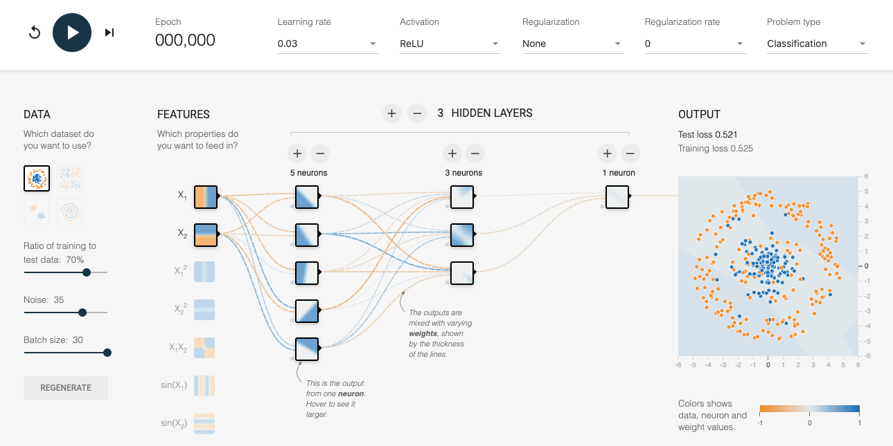
Figure 4-7. Starting point of the spiral classification problem. You can get to this setup by opening up this link in a web browser.
In the playground, we are trying to build a classifier to distinguish between blue dots and orange dots (if you are reading this in the print book, please do follow along by navigating to the link in a web browser). The two input features are x1 and x2, which are the coordinates of the points. Based on these features, the model needs to output the probability that the point is blue. The model starts with random weights and the background of the dots shows the model prediction for each coordinate point. As you can see, because the weights are random, the probability tends to hover near the center value for all the pixels.
Starting the training by clicking on the arrow at the top-left of the image, we see the model slowly start to learn with successive epochs, as shown in Figure 4-8.

Figure 4-8. What the model learns as training progresses. The graphs at the top are the training loss and validation error, while the images show how the model at that stage would predict the color of a point at each coordinate in the grid.
We see the first hint of learning in panel Figure 4-8(b), and see that the model has learned the high-level view of the data by Figure 4-8(c). From then on, the model is adjusting the boundaries to get more and more of the blue points into the center region while keeping the orange points out. This helps, but only up to point. By the time we get to Figure 4-8(e), the adjustment of weights is starting to reflect random perturbations in the training data, and these are counterproductive on the validation dataset.
We can therefore break the training into three phases. In the first phase, between stages (a) and (c), the model is learning high-level organization of the data. In the second phase, between stages and (c) and (e), the model is learning the details. By the time we get to stage (f), we are in the third phase, where the model is overfitting. A partially trained model from the end of phase 1 or from phase 2 has some advantages precisely because it has learned the high-level organization but is not caught up in the details.
Tradeoffs and Alternatives
Besides providing resilience, saving intermediate checkpoints also allows us to implement early stopping and fine tuning capabilities.
Early stopping
In general, the longer you train, the lower the loss on the training dataset. However, at some point, the error on the validation dataset might stop decreasing. If you are starting to overfit to the training dataset, the validation error might even start to increase, as shown in Figure 4-9.
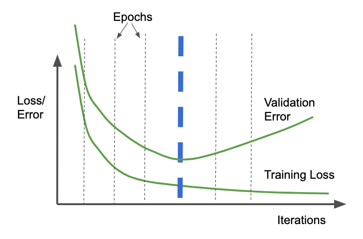
Figure 4-9. Typically, the training loss continues to drop the longer you train, but once overfitting starts, the validation error on a withheld dataset starts to go up.
In such cases, it can be helpful to look at the validation error at the end of every epoch and stop the training process when the validation error is more than that of the previous epoch. In Figure 4-9, this will be at the end of the fourth epoch, shown by the thick dashed line. This is called early stopping.
Note
TIP Had we been checkpointing at the end of every batch, we might have been able to capture the true minimum which might have been a bit before or after the epoch boundary. See the Virtual Epochs design pattern for a more frequent way to checkpoint.
If we are checkpointing much more frequently, it can be helpful if early stopping isn’t overly sensitive to small perturbations in the validation error. Instead, we can apply early stopping only after the validation error doesn’t improve for more than N checkpoints.
Checkpoint selection
While early stopping can be implemented by stopping the training as soon as the validation error starts to increase, we recommend training longer and choosing the optimal run as a post-processing step. The reason we suggest training well into phase 3 (see the preceding “Why It Works” section for an explanation of the three phases of the training loop) is that it is not uncommon for the validation error to increase for a bit and then start to drop again. This is usually because the training initially focuses on more common scenarios (phase 1), and then starts to home in on the rarer situations (phase 2). Because rare situations may be imperfectly sampled between the training and validation datasets, occasional increases in the validation error during the training run are to be expected in phase 2. In addition, there are situations endemic to big models where deep double descent is expected, and so it is essential to train a bit longer just in case.
In our example, instead of exporting the model at the end of the training run, we will load up the fourth checkpoint and export our final model from there instead. This is called checkpoint selection, and in TensorFlow, it can be achieved using BestExporter.
Regularization
Instead of using early stopping or checkpoint selection, it can be helpful to try to add L2 regularization to your model so that the validation error does not increase and so that the model never gets into phase 3. Instead, both the training loss and the validation error should plateau, as shown in Figure 4-10. We term such a training loop (where both training and validation metrics reach a plateau) a well-behaved training loop.
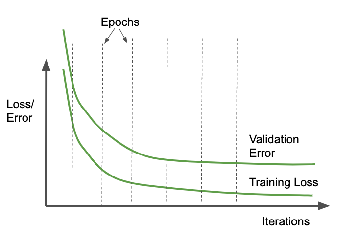
Figure 4-10. In the ideal situation, validation error does not increase. Instead, both the training loss and validation error plateau.
If early stopping is not carried out, and only the training loss is used to decide convergence, then we can avoid having to set aside a separate testing dataset. Even if we are not doing early stopping, displaying the progress of the model training can be helpful, particularly if the model takes a long time to train. Although the performance and progress of the model training is normally monitored on the validation dataset during the training loop, it is for visualization purposes only. Since we don’t have to take any action based on metrics being displayed, we can carry out visualization on the test dataset.
The reason that using regularization might be better than early stopping is that regularization allows you to use the entire dataset to change the weights of the model whereas early stopping requires you to waste 10-20% of your dataset purely to decide when to stop training. Other methods to limit overfitting (such as dropout and using models with lower complexity) are also good alternatives to early stopping. In addition, recent research indicates that double descent happens in a variety of machine learning problems, and therefore it is better to train longer rather than risk a suboptimal solution by stopping early.
Two splits
Isn’t the advice in the regularization section in conflict with the advice in the previous sections on early stopping or checkpoint selection? Not really.
We recommend that you split your data into two parts: a training dataset and an evaluation dataset. The evaluation dataset plays the part of the test dataset during experimentation (where there is no validation dataset) and plays the part of the validation dataset in production (where there is no test dataset).
The larger your training dataset, the more complex a model you can use, and the more accurate a model you can get. Using regularization rather than early stopping or checkpoint selection allows you to use a larger training dataset. In the experimentation phase (when you are exploring different model architectures, training techniques, and hyperparameters), we recommend that you turn off early stopping and train with larger models (See also the Useful Overfitting pattern). This is to ensure that the model has enough capacity to learn the predictive patterns. During this process, monitor error convergence on the training split. At the end of experimentation, you can use the evaluation dataset to diagnose how well your model does on data it has not encountered during training.
When training the model to deploy in production, you will need to prepare to be able to do continuous evaluation and model retraining. Turn on early stopping or checkpoint selection and monitor the error metric on the evaluation dataset. Choose between early stopping and checkpoint selection depending on whether you need to control cost (in which case you would choose early stopping) or want to prioritize model accuracy (in which case you would choose checkpoint selection).
Fine tuning
In a well-behaved training loop, gradient descent behaves such that you get to the neighborhood of the optimal error quickly on the basis of the majority of your data, and then slowly converge towards the lowest error by optimizing on the corner cases.
Now, imagine that you need to periodically retrain the model on fresh data. You typically want to emphasize the fresh data, not the corner cases from last month. You are often better off resuming your training, not from the last checkpoint, but the checkpoint marked by the blue line in Figure 4-11. This corresponds to the start of phase 2 in our discussion of the phases of model training described in the earlier “Why It Works” section. This helps ensure that you have a general method that you are able to then fine-tune for a few epochs on just the fresh data.
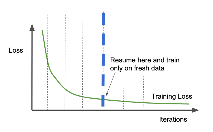
Figure 4-11. Resume from a checkpoint from before the training loss starts to plateau. Train only on fresh data for subsequent iterations.
When you resume from the checkpoint marked by the thick dashed vertical line, you will be on the 4th epoch and so the learning rate will be quite low. Therefore, the fresh data will not dramatically change the model. However, the model will behave optimally (in the context of the larger model) on the fresh data because you will have sharpened it on this smaller dataset. This is called fine tuning. Fine tuning is also discussed in the Transfer Learning design pattern.
Warning
Fine tuning only works as long as you are not changing the model architecture.
It is not necessary to always start from an earlier checkpoint. In some cases, the final checkpoint (that is used to serve the model) can be used as a warm start for another model training iteration. Still, starting from an earlier checkpoint tends to provide better generalization.
Redefining an epoch
Machine learning tutorials often have code like this:
model.fit(X_train, y_train,
          batch_size=100,
          epochs=15)
This code assumes that you have a dataset that fits in memory, and consequently that your model can iterate through 15 epochs without running the risk of machine failure. Both these assumptions are unreasonable — ML datasets range into terabytes, and when training can last hours, the chances of machine failure are high.
To make the preceding code more resilient, supply a tf.dataset (not just a numpy array) because the tf.dataset is an out-of-memory dataset. It provides iteration capability and lazy loading. The code is now as follows:
cp_callback = tf.keras.callbacks.ModelCheckpoint(...)
history = model.fit(trainds,
                    validation_data=evalds,
                    epochs=15,
                    batch_size=128,
                    callbacks=[cp_callback])
However, using epochs on large datasets remains a bad idea. Epochs may be easy to understand, but the use of epochs leads to bad effects in real-world ML models. Too see why, imagine that you have a training dataset with 1 million examples. It can be tempting to simply go through this dataset 15 times (for example) by setting the number of epochs to 15. There are several problems with this:
-
The number of epochs is an integer, but the difference in training time between processing the dataset 14.3 times and 15 times can be hours. If the model has converged after having seen 14.3 million examples, you might want to exit and not waste the computational resources necessary to process 0.7 million more examples.
-
You checkpoint once per epoch and waiting 1 million examples between checkpoints might be way too long. For resilience, you might want to checkpoint more often.
-
Datasets grow over time. If you get 100,000 more examples and you train the model and get a higher error, is it because you need to do an early stop or is the new data corrupt in some way? You can’t tell because the prior training was on 15 million examples and the new one is on 16.5 million examples.
-
In distributed, parameter-server training (See Distribution Strategy) with data parallelism and proper shuffling, the concept of an epoch is not clear anymore. Because of potentially straggling workers, you can only instruct the system to train on some number of mini-batches.
Steps per epoch
Instead of training for 15 epochs, we might decide to train for 143,000 steps where the batch_size is 100:
NUM_STEPS = 143000
BATCH_SIZE = 100
NUM_CHECKPOINTS = 15
cp_callback = tf.keras.callbacks.ModelCheckpoint(...)
history = model.fit(trainds,
                    validation_data=evalds,
                    epochs=NUM_CHECKPOINTS,
                    steps_per_epoch=NUM_STEPS // NUM_CHECKPOINTS,
                    batch_size=BATCH_SIZE,
                    callbacks=[cp_callback])
Each step involves weight updates based on a single mini-batch of data and this allows us to stop at 14.3 epochs. This gives us much more granularity, but we have to define an “epoch” as 1/15th of the total number of steps:
steps_per_epoch=NUM_STEPS // NUM_CHECKPOINTS,
This is so that we get the right number of checkpoints. It works as long as we make sure to repeat the trainds infinitely:
trainds = trainds.repeat()
The repeat() is needed because we no longer set num_epochs, so the number of epochs defaults to one. Without the repeat(), the model will exit once the training patterns are exhausted after reading the dataset once.
Retraining with more data
What happens when we get 100,000 more examples? Easy! We add it to our data warehouse but do not update the code. Our code will still want to process 143,000 steps and it will get to process that much data, except that 10% of the examples it sees are newer. If the model converges, great. If it doesn’t, we know that these new data points are the issue because we are not training longer than we were before. By keeping the number of steps constant, we have been able to separate out the effects of new data from training on more data.
Once we have trained for 143,000 steps, we restart the training and run it a bit longer (say, 10,000 steps) and as long as the model continues to converge, we keep training it longer. Then, we update the number 143,000 in the code above (in reality, it will be a parameter to the code) to reflect the new number of steps.
This all works fine, until you want to do hyperparameter tuning. When you do hyperparameter tuning, you will want to want to change the batch size. Unfortunately, if you change the batch size to 50, you will find yourself training for half the time because we are training for 143,000 steps, and each step is only half as long as before. Obviously, this is no good.
Virtual epochs
The answer is to keep the total number of training examples shown to the model (not number of steps, see Figure 4-12) constant:
NUM_TRAINING_EXAMPLES = 1000 * 1000
STOP_POINT = 14.3
TOTAL_TRAINING_EXAMPLES = int(STOP_POINT * NUM_TRAINING_EXAMPLES)
BATCH_SIZE = 100
NUM_CHECKPOINTS = 15
steps_per_epoch = (TOTAL_TRAINING_EXAMPLES //
                   (BATCH_SIZE*NUM_CHECKPOINTS))
cp_callback = tf.keras.callbacks.ModelCheckpoint(...)
history = model.fit(trainds,
                    validation_data=evalds,
                    epochs=NUM_CHECKPOINTS,
                    steps_per_epoch=steps_per_epoch,
                    batch_size=BATCH_SIZE,
                    callbacks=[cp_callback])
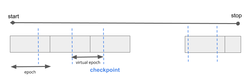
Figure 4-12. Defining a virtual epoch in terms of the desired number of steps between checkpoints.
When you get more data, first train it with the old settings, then increase the number of examples to reflect the new data, and finally change the STOP_POINT to reflect the number of times you have to traverse the data to attain convergence.
This is now safe even with hyperparameter tuning (discussed later in this chapter) and retains all the advantages of keeping the number of steps constant.
Design Pattern 13: Transfer Learning
In Transfer Learning, we take part of a previously trained model, freeze the weights, and incorporate these non-trainable layers into a new model that solves a similar problem, but on a smaller dataset.
Problem
Training custom ML models on unstructured data requires extremely large datasets, which are not always readily available. Consider the case of a model identifying whether an x-ray of an arm contains a broken bone. To achieve high accuracy, you’ll need hundreds of thousands of images if not more. Before your model learns what a broken bone looks like, it needs to first learn to make sense of the pixels, edges, and shapes that are part of the images in your dataset. The same is true for models trained on text data. Let’s say we’re building a model that takes descriptions of patient symptoms and predicts the possible conditions associated with those symptoms. In addition to learning which words differentiate a cold from pneumonia, the model also needs to learn basic language semantics and how the sequence of words creates meaning. For example, the model would need to not only learn to detect the presence of the word fever, but that the sequence no fever carries a very different meaning than high fever.
To see just how much data is required to train high accuracy models, we can look at ImageNet, a database of over 14 million labeled images. ImageNet is frequently used as a benchmark for evaluating machine learning frameworks on various hardware. For example, according to Stanford’s DAWNBench model benchmarking suite, TensorFlow 2 (in 2020) took just over two and a half minutes to reach 93% accuracy on Imagenet when trained on a GPU. With more training time, models can reach even higher accuracy on ImageNet. However, this is largely due to ImageNet’s size. Most organizations with specialized prediction problems don’t have nearly as much data available.
Because use cases like the image and text examples described above involve particularly specialized data domains, it’s also not possible to use a general-purpose model to successfully identify bone fractures or diagnose diseases. A model that is trained on ImageNet might be able to label an x-ray image as x-ray or medical imaging but is unlikely to be able to label it as a broken femur. Because such models are often trained on a wide variety of high level label categories, we wouldn’t expect them to understand conditions present in the images that are specific to our dataset. To handle this, we need a solution that allows us to build a custom model using only the data we have available and with the labels that we care about.
Solution
With the Transfer Learning design pattern, we can take a model that has been trained on the same type of data for a similar task and apply it to a specialized task using our own custom data. By “same type of data,” we mean the same data modality – images, text, and so forth. Beyond just the broad category like images, it is also ideal to use a model that has been pre-trained on the same types of images. For example, use a model that has been pre-trained on photographs if you are going to use it for photograph classification and a model that has been pre-trained on remotely sensed imagery if you are going to use it to classify satellite images. By similar task, we’re referring to the problem being solved. To do transfer learning for image classification, for example, it is better to start with a model that has been trained for image classification, rather than object detection.
Continuing with the example, let’s say we’re building a binary classifier to determine whether an image of an x-ray contains a broken bone. We only have 200 images of each class: broken and not broken. This isn’t enough to train a high quality model from scratch, but it is sufficient for transfer learning. To solve this with transfer learning, we’ll need to find a model that has already been trained on a large dataset to do image classification. We’ll then remove the last layer from that model, freeze the weights of that model, and continue training using our 400 x-ray images. We’d ideally find a model trained on a dataset with similar images to our x-rays, like images taken in a lab or another controlled condition. However, we can still utilize transfer learning if the datasets are different, so long as the prediction task is the same. In this case we’re doing image classification.
We can use transfer learning for many prediction tasks in addition to image classification, so long as there is an existing pre-trained model that matches the task you’d like to perform on your dataset. For example, transfer learning is also frequently applied in image object detection, image style transfer, image generation, text classification, machine translation, and more.
Note
Transfer learning works because it lets us stand on the shoulders of giants, utilizing models that have already been trained on extremely large, labeled datasets. We’re able to use transfer learning thanks to years of research and work others have put into creating these datasets for us, which has advanced the state-of-the-art in transfer learning. One example of such a dataset is the ImageNet project, started in 2006 by Fei-Fei Li and published in 2009. ImageNet2 has been essential to the development of transfer learning, and paved the way for other large datasets like COCO and Open Images.
The idea behind transfer learning is that you can utilize the weights and layers from a model trained in the same domain as your prediction task. In most deep learning models, the final layer contains the classification label or output specific to your prediction task. With transfer learning, we remove this layer, freeze the model’s trained weights, and replace the final layer with the output for our specialized prediction task before continuing to train. We can see how this works in Figure 4-13.
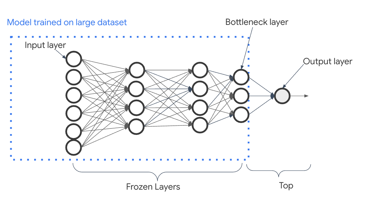
Figure 4-13. Transfer learning involves training a model on a large dataset. The “top” of the model (typically, just the output layer) is removed and the remaining layers have their weights frozen. The last layer of the remaining model is called the bottleneck layer.
Typically, the penultimate layer of the model (the layer before the model’s output layer) is chosen as the bottleneck layer. Next we’ll explain the bottleneck layer, along with different ways to implement transfer learning in TensorFlow.
Bottleneck layer
In relation to an entire model, the bottleneck layer represents the input (typically an image or text document) in the lowest dimensionality space. More specifically, when we feed data into our model, the first layers see this data nearly in its original form. To see how this works, let’s continue with a medical imaging example, but this time we’ll build a model with a colorectal histology dataset to classify the histology images into one of eight categories.
To explore the model we are going to use for transfer learning, let’s load the VGG model architecture pre-trained on the ImageNet dataset:
vgg_model_withtop = tf.keras.applications.VGG19(include_top=True,weights='imagenet',)
Notice that we’ve set include_top=True, which means we’re loading the full VGG model including the output layer. For ImageNet, the model classifies images into 1000 different classes, so the output layer is a 1000-element array. Let’s look at the output of model.summary() to understand which layer will be used as the bottleneck. For brevity, we’ve left out some of the middle layers here:
Model: "vgg19"_________________________________________________________________Layer (type) Output Shape Param #=================================================================input_3 (InputLayer) [(None, 224, 224, 3)] 0_________________________________________________________________block1_conv1 (Conv2D) (None, 224, 224, 64) 1792…more layers here..._________________________________________________________________block5_conv3 (Conv2D) (None, 14, 14, 512) 2359808_________________________________________________________________block5_conv4 (Conv2D) (None, 14, 14, 512) 2359808_________________________________________________________________block5_pool (MaxPooling2D) (None, 7, 7, 512) 0_________________________________________________________________flatten (Flatten) (None, 25088) 0_________________________________________________________________fc1 (Dense) (None, 4096) 102764544_________________________________________________________________fc2 (Dense) (None, 4096) 16781312_________________________________________________________________predictions (Dense) (None, 1000) 4097000=================================================================Total params: 143,667,240Trainable params: 143,667,240Non-trainable params: 0_________________________________________________________________
As you can see, the VGG model accepts images as a 224x224x3 pixel array. This 128-element array is then passed through successive layers (each of which may change the dimensionality of the array) until it is flattened into a 25088x1-dimensional array in the layer called flatten. Finally, it is fed into the output layer, which returns a 1000-element array (for each class in ImageNet). In this example, we’ll choose the block5_pool layer as the bottleneck layer when we adapt this model to be trained on our medical histology images. The bottleneck layer produces a 7x7x512-dimensional array, which is a low dimensional representation of the input image. It has retained enough of the information from the input image to be able to classify it. When we apply this model to our medical image classification task, we hope that the information distillation will be sufficient to successfully carry out classification on our dataset.
The histology dataset comes with images as (150,150,3) dimensional arrays. This 150x150x3 representation is the highest dimensionality. To use the VGG model with our image data, we can load it with the following:
vgg_model = tf.keras.applications.VGG19(include_top=False,weights='imagenet',input_shape=((150,150,3)))vgg_model.trainable = False
By setting include_top=False, we’re specifying that the last layer of VGG we want to load is the bottleneck layer. The input_shape we passed in matches the input shape of our histology images. A summary of the last few layers of this updated VGG model looks like the following:
block5_conv3 (Conv2D) (None, 9, 9, 512) 2359808_________________________________________________________________block5_conv4 (Conv2D) (None, 9, 9, 512) 2359808_________________________________________________________________block5_pool (MaxPooling2D) (None, 4, 4, 512) 0=================================================================Total params: 20,024,384Trainable params: 0Non-trainable params: 20,024,384_________________________________________________________________
The last layer is now our bottleneck layer. You may notice that the size of block5_pool is (4,4,512) whereas before it was (7,7,512). This is because we instantiated VGG with an input_shape parameter to account for the size of the images in our dataset. It’s also worth noting that setting include_top=False is hardcoded to use block5_pool as the bottleneck layer, but if you want to customize this you can load the full model and delete any additional layers you don’t want to use.
Before this model is ready to be trained, we’ll need to add a few layers on top, specific to our data and classification task. It’s also important to note that because we’ve set trainable=False, there are 0 trainable parameters in the current model.
Note
TIP As a general rule of thumb, the bottleneck layer is typically the last, lowest dimensionality, flattened layer before a flattening operation.
Because they both represent features in reduced dimensionality, bottleneck layers are conceptually similar to embeddings. For example, in an autoencoder model with an encoder-decoder architecture, the bottleneck layer is an embedding. In this case the bottleneck serves as the middle layer of the model, mapping the original input data to a lower-dimensionality representation, which the decoder (the second half of the network) uses to map the input back to its original, higher dimensional representation. To see a diagram of the bottleneck layer in an autoencoder, refer to Figure 2-13 in Chapter 2.
An embedding layer is essentially a lookup table of weights, mapping a particular feature to some dimension in vector space. The main difference is that the weights in an embedding layer can be trained, whereas all the layers leading up to and including the bottleneck layer have their weights frozen. In other words, the entire network up to and including the bottleneck layer is non-trainable, and the weights in the layers after the bottleneck are the only trainable layers in the model.
Note
It’s also worth noting that pre-trained embeddings can be used in the Transfer Learning design pattern. When you build a model that includes an embedding layer, you can either utilize an existing (pre-trained) embedding lookup, or train your own embedding layer from scratch.
To summarize, transfer learning is a solution you can employ to solve a similar problem on a smaller dataset. Transfer learning always makes use of a bottleneck layer with non-trainable, frozen weights. Embeddings are a type of data representation. Ultimately, it comes down to purpose. If the purpose is to train a similar model, you would use transfer learning. Consequently, if the purpose is to represent an input image more concisely, you would use an embedding. The code might be exactly the same.
Implementing transfer learning
You can implement transfer learning in Keras using one of these two methods:
-
Loading a pre-trained model on your own, removing the layers after the bottleneck, and adding a new final layer with your own data and labels
-
Using a pre-trained TensorFlow Hub module as the foundation for your transfer learning task
Let’s start by looking at how to load and use a pre-trained model on your own. For this we’ll build on the VGG model example we introduced earlier. Note that VGG is a model architecture, whereas ImageNet is the data it was trained on. Together, these make up the pre-trained model we’ll be using for transfer learning. Here, we’re using transfer learning to classify colorectal histology images. Whereas the original ImageNet dataset contains 1000 labels, our resulting model will only return eight possible classes that we’ll specify, as opposed to the thousands of labels present in ImageNet.
Note
Loading a pre-trained model and using it to get classifications on the original labels that model was trained on is not transfer learning. Transfer learning is going one step further, replacing the final layers of the model with your own prediction task.
The VGG model we’ve loaded will be our base model. We’ll need to add a few layers to flatten the output of our bottleneck layer, and feed this flattened output into an 8-element softmax array:
global_avg_layer = tf.keras.layers.GlobalAveragePooling2D()feature_batch_avg = global_avg_layer(feature_batch)prediction_layer = tf.keras.layers.Dense(8, activation='softmax')prediction_batch = prediction_layer(feature_batch_avg)
Finally, we can use the Sequential API to create our new transfer learning model as a stack of layers:
histology_model = keras.Sequential([vgg_model,global_avg_layer,prediction_layer])
Let’s take note of the output of model.summary() on our transfer learning model:
_________________________________________________________________Layer (type) Output Shape Param #=================================================================vgg19 (Model) (None, 4, 4, 512) 20024384_________________________________________________________________global_average_pooling2d (Gl (None, 512) 0_________________________________________________________________dense (Dense) (None, 8) 4104=================================================================Total params: 20,028,488Trainable params: 4,104Non-trainable params: 20,024,384_________________________________________________________________
The important piece here is that the only trainable parameters are the ones after our bottleneck layer. In this example, the bottleneck layer is the feature vectors from the VGG model. After compiling this model, we can train it by feeding it our dataset of histology images.
Pretrained embeddings
While we can load a pre-trained model on our own, we can also implement transfer learning by making use of the many pre-trained models available in TF Hub, a library of pre-trained models (called modules). These modules span a variety of data domains and use cases, including classification, object detection, machine translation, and more. In Tensorflow, you can load these modules as a layer, and then add your own classification layer on top.
To see how TF Hub works, let’s build a model that classifies movie reviews as either positive or negative. First, we’ll load a pre-trained embedding model trained on a large corpus of news articles. We can instantiate this model as a hub.KerasLayer:
hub_layer = hub.KerasLayer("https://tfhub.dev/google/tf2-preview/gnews-swivel-20dim/1",input_shape=[], dtype=tf.string, trainable=True)
We can stack additional layers on top of this to build our classifier:
model = keras.Sequential([hub_layer,keras.layers.Dense(32, activation='relu'),keras.layers.Dense(1, activation='sigmoid')])
We can now train this model, passing it our own text dataset as input. The resulting prediction will be a 1-element array indicating whether our model thinks the given text is positive or negative.
Why It Works
To understand why transfer learning works, let’s first look at an analogy. When children are learning their first language, they are exposed to many examples and corrected if they misidentify something. For example, the first time they learn to identify a cat they’ll see their parents point to the cat and say the word cat, and this repetition strengthens pathways in their brain. Similarly, they are corrected when they say cat referring to an animal that is not a cat. When the child then learns how to identify a dog, they don’t need to start from scratch. They can use a similar recognition process to the one they used for the cat, but apply it to a slightly different task. In this way, the child has built a foundation for learning. In addition to learning new things, they have also learned how to learn new things. Applying these learning methods to different domains is roughly how transfer learning works too.
How does this play out in neural networks? In a typical Convolutional Neural Network (CNN), the learning is hierarchical. The first layers learn to recognize edges and shapes present in an image. In the cat example, this might mean the model can identify areas in an image where the edge of the cat’s body meets the background. The next layers in the model begin to understand groups of edges – perhaps that there are two edges that meet towards the top left corner of the image. A CNN’s final layers can then piece together these groups of edges, developing an understanding of different features in the image. In the cat example, the model might be able to identify two triangular shapes towards the top of the image and two oval shapes below them. As humans, we know that these triangular shapes are ears and the oval shapes are eyes.
We can visualize this process in Figure 4-14, from research by Zeller and Fergus on deconstructing CNNs to understand the different features that were activated throughout each layer of the model. For each layer in a 5-layer CNN, this shows an image’s feature map for a given layer alongside the actual image. This lets us see how the model’s perception of an image progresses as it moves throughout the network. Layer 1 and 2 recognize only edges, layer 3 begins to recognize objects, and layers 4-5 can understand focal points within the entire image.
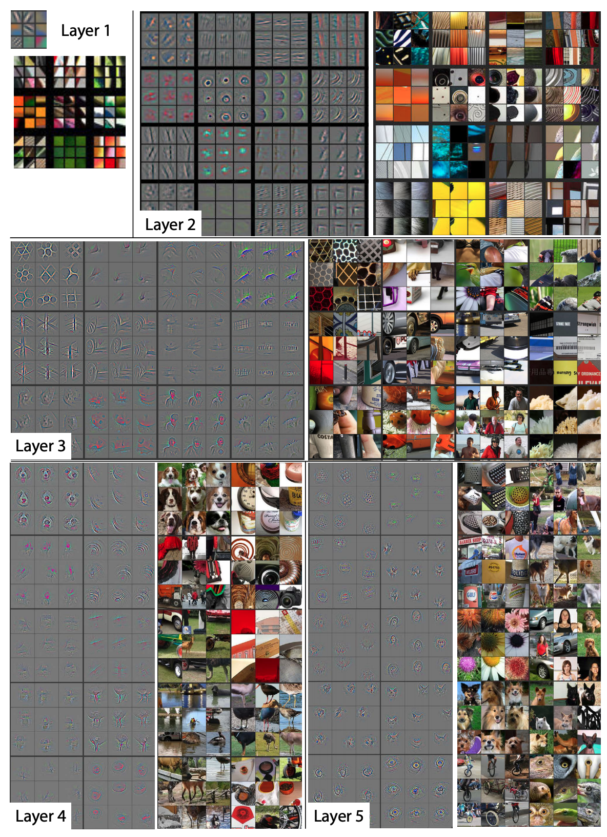
Figure 4-14. Research from Zeiler and Fergus (2013) in deconstructing CNNs helps us visualize how a CNN sees images at each layer of the network.
Remember, though, that to our model these are simply groupings of pixel values. It doesn’t know that the triangular and oval shapes are ears and eyes – it only knows to associate specific groupings of features with the labels it has been trained on. In this way, the model’s process of learning what groupings of features make up a cat isn’t much different from learning the groups of features that are part of other objects, like a table, a mountain, or even a celebrity. To a model these are all just different combinations of pixel values, edges, and shapes.
Tradeoffs and Alternatives
So far, we haven’t discussed methods of modifying the weights of our original model when implementing transfer learning. Here we’ll examine two approaches for this: feature extraction and fine-tuning. We’ll also discuss why transfer learning is primarily focused on image and text models, and look at the relationship between text sentence embeddings and transfer learning.
Fine-tuning vs. feature extraction
Feature extraction describes an approach to transfer learning where you freeze the weights of all layers before the bottleneck layer, and train the following layers on your own data and labels. Another option is instead fine-tuning the weights of the pre-trained model’s layers. With fine-tuning, you can either update the weights of each layer in the pre-trained model, or just a few of the layers right before the bottleneck. Training a transfer learning model using fine-tuning typically takes longer than feature extraction. You’ll notice in our text classification example above, we set trainable=True when initializing our TF Hub layer. This is an example of fine-tuning.
When fine-tuning, it’s common to leave the weights of the model’s initial layers frozen since these layers have been trained to recognize basic features which are often common across many types of images. To fine-tune a MobileNet model, for example, we’d set trainable=False only for a subset of layers in the model, rather than making every layer non-trainable. For example, to fine-tune after the 100th layer, we could run:
base_model = tf.keras.applications.MobileNetV2(input_shape=(160,160,3),include_top=False,weights='imagenet')for layer in base_model.layers[:100]:layer.trainable = False
One recommended approach to determining how many layers to freeze is known as progressive fine-tuning3, and involves iteratively unfreezing layers after every training run to find the ideal number of layers to fine-tune. This works best and is most efficient if you keep your learning rate low (0.001 is common) and the number of training iterations relatively small. To implement progressive fine-tuning, start by unfreezing only the last layer of your transferred model (the layer closest to the output) and calculate your model’s loss after training. Then, one by one unfreeze more layers until you reach the input layer or until the loss starts to plateau. Use this to inform the number of layers to fine-tune.
How should you determine whether to fine-tune or freeze all layers of your pre-trained model? Typically, when you’ve got a small dataset, it’s best to use the pre-trained model as a feature extractor rather than fine-tuning. If you’re re-training the weights of a model that was likely trained on thousands or millions of examples, fine-tuning can cause the updated model to overfit to your small dataset and lose the more general information learned from those millions of examples. Although it depends on your data and prediction task, when we say “small dataset” here we’re referring to datasets with hundreds or a few thousand training examples.
Another factor to take into account when deciding whether to fine-tune is how similar your prediction task is to that of the original pre-trained model you’re using. When the prediction task is similar or a continuation of the previous training, as it was in our movie review sentiment analysis model, fine-tuning can produce higher accuracy results. When the task is different or the datasets are significantly different, it’s best to freeze all the layers of the pre-trained model instead of fine-tune them. Table 4-1 summarizes the key points.4
Table 4-1. Criteria to help choose between feature extraction and fine tuning.
| Criterion | Feature extraction | Fine tuning |
| How large is the dataset? | Small | Large |
| Is your prediction task the same as that of the pre-trained model? | Different tasks | Same task, or similar task with same class distribution of labels |
| Budget for training time and computational cost | Low | High |
In our text example, the pre-trained model was trained on a corpus of news text but our use case was sentiment analysis. Because these tasks are different, we should use the original model as a feature extractor rather than fine-tune it. An example of different prediction tasks in an image domain might be using our MobileNet model trained on ImageNet as a basis for doing transfer learning on a dataset of medical images. Although both tasks involve image classification, the nature of the images in each dataset are very different.
Focus on image and text models
You may have noticed that all of the examples in this section focused on image and text data. This is because transfer learning is primarily for cases where you can apply a similar task to the same data domain. Models trained with tabular data, however, cover a potentially infinite number of possible prediction tasks and data types. You could train a model on tabular data to predict how you should price tickets to your event, whether or not someone is likely to default on loan, your company’s revenue next quarter, the duration of a taxi trip, and so forth. The specific data for these tasks is also incredibly varied, with the ticket problem depending on information about artists and venues, the loan problem on personal income, and the taxi duration on urban traffic patterns. For these reasons, there are inherent challenges in transferring the learnings from one tabular model to another.
Although transfer learning is not yet as common on tabular data as it is for image and text domains, a new model architecture called TabNet presents novel research in this area. Most tabular models require significant feature engineering when compared with image and text models. TabNet employs a technique that first uses unsupervised learning to learn representations for tabular features, and then fine-tunes these learned representations to produce predictions. In this way, TabNet automates feature engineering for tabular models.
Embeddings of words vs. sentences
In our discussion of text embeddings so far, we’ve referred mostly to word embeddings. Another type of text embedding is sentence embeddings. Where word embeddings represent individual words in vector space, sentence embeddings do similar but with entire sentences. Consequently, word embeddings are context agnostic. Let’s see how this plays out with the following sentence:
“I’ve left you fresh baked cookies on the left side of the kitchen counter.”
Notice that the word left appears twice in that sentence, first as a verb and then as an adjective. If we were to generate word embeddings for this sentence, we’d get a separate array for each word. With word embeddings, the array for both instances of the word left would be the same. Using sentence-level embeddings, however, we’d get a single vector to represent the entire sentence. There are several approaches for generating sentence embeddings – from averaging a sentence’s word embeddings to training a supervised learning model on a large corpus of text to generate the embeddings.
How does this relate to transfer learning? The latter method – training a supervised learning model to generate sentence-level embeddings – is actually a form of transfer learning. This is the approach used by Google’s Universal Sentence Encoder (available in TF Hub) and BERT. These methods differ from word embeddings in that they go beyond simply providing a weight lookup for individual words. Instead, they have been built by training a model on a large dataset of varied text to understand the meaning conveyed by sequences of words. In this way, they are designed to be transferred to different natural language tasks and can thus be used to build models that implement transfer learning.
Design Pattern 14: Distribution Strategy
In Distribution Strategy, the training loop is carried out at scale over multiple workers, often with caching, hardware acceleration, and parallelization.
Problem
These days, it’s common for large neural networks to have millions of parameters and be trained on massive amounts of data. In fact, it’s been shown that increasing the scale of deep learning, with respect to the number of training examples, the number of model parameters, or both, drastically improves model performance. However, as the size of models and data increases, the computation and memory demands increase proportionally, making the time it takes to train these models one of the biggest problems of deep learning.
GPUs provide a substantial computational boost and bring the training time of modestly sized deep neural networks within reach. However, for very large models trained on massive amounts of data, individual GPUs aren’t enough to make the training time tractible. For example, at the time of writing, training ResNet-50 on the benchmark ImageNet dataset for 90 epochs on a single NVIDIA M40 GPU requires 10^18 single precision operations and takes 14 days. As AI is being used more and more to solve problems within complex domains, and open source libraries like Tensorflow and PyTorch make building deep learning models more accessible, large neural networks comparable to ResNet-50 have become the norm.
This is a problem. If it takes two weeks to train your neural network, then you have to wait two weeks before you can iterate on new ideas or experiment with tweaking the settings. Furthermore, for some complex problems like medical imaging, autonomous driving, or language translation, it’s not always feasible to break the problem down into smaller components or work with only a subset of the data. It’s only with the full scale of the data that you can assess whether things work or not.
Training time translates quite literally to money. In the world of serverless machine learning, rather than buying your own expensive GPU, it is possible to submit training jobs via a cloud service where you are charged for training time. The cost of training a model, whether it is to pay for a GPU or to pay for a serverless training service, quickly adds up.
Is there a way to speed up the training of these large neural networks?
Solution
One way to accelerate training is through distribution strategies in the training loop. There are different distribution techniques but the common idea is to split the effort of training the model across multiple machines. There are two ways this can be done: data parallelism and model parallelism. In data parallelism, computation is split across different machines and different workers train on different subsets of the training data. In model parallelism, the model is split and different workers carry out the computation for different parts of the model. In this section we’ll focus on data parallelism and show implementations in TensorFlow using the tf.distribute.Strategy library. We’ll discuss model parallelism in the section on Tradeoffs and Alternatives.
To implement data parallelism, there must be a method in place for different workers to compute gradients and share that information to make updates to the model parameters. This ensures that all workers are consistent and each gradient step works to train the model. Broadly speaking, data parallelism can be carried out either synchronously or asynchronously.
Synchronous training
In synchronous training, the workers train on different slices of input data in parallel and the gradient values are aggregated at the end of each training step. This is performed via an all-reduce algorithm. This means that each worker, typically a GPU, has a copy of the model on device and, for a single Stochastic Gradient Descent (SGD) step, a mini-batch of data is split amongst each of the separate workers. Each device performs a forward pass with their portion of the mini-batch and computes gradients for each parameter of the model. These locally computed gradients are then collected from each device and aggregated (for example, averaged) to produce a single gradient update for each parameter. A central server holds the most current copy of the model parameters and performs the gradient step according to the gradients received from the multiple workers. Once the model parameters are updated according to this aggregated gradient step, the new model is sent back to the workers along with another split of the next mini-batch and the process repeats. Figure 4-15 shows a typical all-reduce architecture for synchronous data distribution.

Figure 4-15. In synchronous training each worker holds a copy of the model and computes gradients using a slice of the training data mini-batch.
As with any parallelism strategy, this introduces additional overhead to manage timing and communication between workers. Large models could cause I/O bottlenecks as data is passed from the CPU to the GPU during training and slow networks could also cause delays.
In Tensorflow, tf.distribute.MirroredStrategy supports synchronous distributed training across multiple GPUs on the same machine. Each model parameter is mirrored across all workers and stored as a single conceptual variable called MirroredVariable. During the all-reduce step, all gradient tensors are made available on each device. This helps to significantly reduce the overhead of synchronization. There are also various other implementations for the all-reduce algorithm available, many of which use NVIDIA NCCL.
To implement this mirrored strategy in Keras, you first create an instance of the mirrored distribution strategy, and then move the creation and compiling of the model inside the scope of that instance. The following code shows how to use MirroredStrategy when training a 3-layer neural network:
mirrored_strategy = tf.distribute.MirroredStrategy()with mirrored_strategy.scope():model = tf.keras.Sequential([tf.keras.layers.Dense(32, input_shape=(5,)),tf.keras.layers.Dense(16, activation='relu'),tf.keras.layers.Dense(1)])model.compile(loss='mse', optimizer='sgd')
By creating the model inside this scope, the parameters of the model are created as mirrored variables instead of regular variables. When it comes to fitting the model on the dataset, everything is performed exactly the same as before. The model code stays the same! Wrapping the model code in the distribution strategy scope is all you need to do to enable distributed training. The MirroredStrategy handles replicating the model parameters on the available GPUs, aggregating gradients, and more. To train or evaluate the model we just call .fit or .evaluate as usual:
model.fit(train_dataset, epochs=2)model.evaluate(train_dataset)
During training, each batch of the input data is divided equally among the multiple workers. For example, if you are using two GPUs, then a batch size of 10 will be split among the two GPUs with each receiving 5 training examples each step.
There are also other synchronous distribution strategies within Keras such as CentralStorageStrategy and MultiWorkerMirroredStrategy. MultiWorkerMirroredStrategy enables the distribution to be spread not just on GPUs on a single machine, but on multiple machines. In CentralStorageStrategy the model variables are not mirrored, instead they are placed on the CPU and operations are replicated across all local GPUs. So the variable updates only happen in one place.
When choosing between different distribution strategies, the best option depends on your computer topology and how fast the CPUs and GPUs can communicate with each other. Table 4-2 summarizes how the different strategies described here compare on these criteria.
Table 4-2. Choosing between distribution strategies depends on your computer topology and how fast the CPUs and GPUs can communicate with each other
| Faster CPU-GPU connection | Faster GPU-GPU connection | |
| One machine with multiple GPUs |
CentralStorageStrategy
|
MirroredStrategy
|
| Multiple machines with multiple GPUs |
MultiWorkerMirroredStrategy
|
|
Asynchronous training
In asynchronous training, the workers train on different slices of the input data independently, and the model weights and parameters are updated asynchronously, typically through a parameter server architecture. This means that no one worker waits for updates to the model from any of the other workers. In the parameter-server architecture there is a single parameter server which manages the current values of the model weights, as in Figure 4-16.
As with synchronous training, a mini-batch of data is split amongst each of the separate workers for each SGD step. Each device performs a forward pass with their portion of the mini-batch and computes gradients for each parameter of the model. Those gradients are sent to the parameter server which performs the parameter update and then sends the new model parameters back to the worker with another split of the next mini-batch.
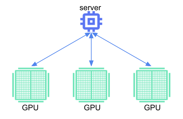
Figure 4-16. In asynchronous training, each worker performs a gradient descent step with a split of the mini-batch. No one worker waits for updates to the model from any of the other workers.
The key difference between synchronous and asynchronous training is that the parameter server does not do an all-reduce. Instead, it computes the new model parameters periodically based on whichever gradient updates it received since the last computation. Typically, asynchronous distribution achieves higher throughput than synchronous training because a slow worker doesn’t block the progression of training steps. If a single worker fails, the training continues as planned with the other workers while that worker reboots. As a result, some splits of the mini-batch may be lost during training, making it too difficult to accurately keep track of how many epochs of data have been processed. This is one reason why we typically specify virtual epochs when training large distributed jobs instead of epochs; see the Checkpoints design pattern in this chapter for a discussion of Virtual Epochs.
In addition, since there is no synchronization between the weight updates, it is possible that one worker updates the model weights based on stale model state. However, in practice this doesn’t seem to be a problem. Typically, large neural networks are trained for multiple epochs and these small discrepancies become negligible in the end.
In Keras, ParameterServerStrategy implements asynchronous parameter server training on multiple machines. When using this distribution, some machines are designated as workers and some are held as parameter servers. The parameter servers hold each variable of the model and computation is performed on the workers, typically GPUs.
The implementation is similar to that of other distribution strategies in Keras. For example in your code, you would just replace MirroredStrategy() with ParameterServerStrategy().
Note
TIP Another distribution strategy supported in Keras worth mentioning is OneDeviceStrategy. This strategy will place any variables created in its scope on the specified device. This strategy is particularly useful as a way to test your code before switching to other strategies which actually distribute to multiple devices/machines.
Synchronous and asynchronous training each have their advantages and disadvantages and choosing between the two often comes down to hardware and network limitations.
Synchronous training is particularly vulnerable to slow devices or poor network connection because training will stall waiting for updates from all workers. This means synchronous distribution is preferable when all devices are on a single host and there are fast devices (for example, TPUs or GPUs) with strong links. On the other hand, asynchronous distribution is preferable if there are many low-power or unreliable workers. If a single worker fails or stalls in returning a gradient update, it won’t stall the training loop. The only limitation is I/O constraints.
Why It Works
Large, complex neural networks require massive amounts of training data to be effective. Distributed training schemes drastically increase the throughput of data processed by these models and can effectively decrease training times from weeks to hours. Sharing resources between workers and parameter server tasks leads to a dramatic increase in data throughput. Figure 4-17 compares the throughput of training data, in this case images, with different distribution setups. Most notable is that throughput increases with the number of worker nodes and, even though parameter servers perform tasks not related to the computation done on the GPUs workers, splitting the workload among more machines is the most advantageous strategy.
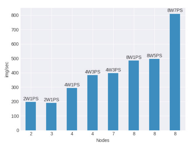
Figure 4-17. Comparison of throughput between different distribution setups. Here, 2W1PS indicates 2 workers and 1 parameter server.5
In addition, data parallelization decreases time to convergence during training. In a similar study, it was shown that increasing workers leads to minimum loss much faster. Figure 4-18 compares the time to minimum for different distribution strategies. As the number of workers increases, the time to minimum training loss dramatically decreases showing nearly a 5x speed up with 8 workers as opposed to just 1.
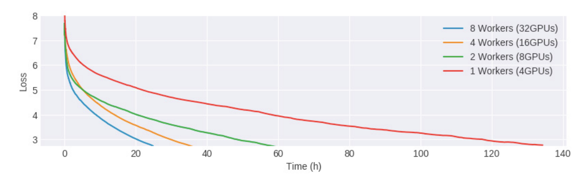
Figure 4-18. As the number of GPUs increases, the time to convergence during training decreases.6
Tradeoffs and Alternatives
In addition to data parallelism there are other aspects of distribution to consider, such as model parallelism, other training accelerators, such as TPUs, and other considerations, such as I/O limitations and batch size.
Model parallelism
In some cases the neural network is so large it cannot fit in the memory of a single device; for example, Google’s Neural Machine Translation has billions of parameters. In order to train models this big, they must be split up over multiple devices, as shown in Figure 4-19. This is called model parallelism. By partitioning parts of a network and their associated computations across multiple cores, the computation and memory workload is distributed across multiple devices. Each device operates over the same mini-batch of data during training, but carrying out computations related only to their separate components of the model.
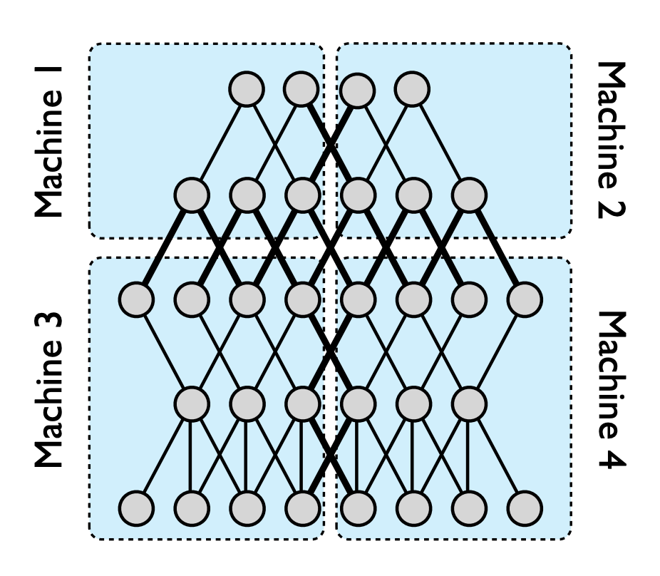
Figure 4-19. Model parallelism partitions the model over multiple devices7.
ASICs for better performance at lower cost
Another way to speed up the training process is by accelerating the underlying hardware such as by using Application Specific Integrated Circuits (ASICs). In machine learning, this refers to hardware components designed specifically to optimize performance on the types of large matrix computations at the heart of the training loop. TPUs in Google Cloud are ASICs that can be used for both model training and making predictions. Similarly, Microsoft Azure offers the Azure FPGA (Field-Programmable Gate Array) which is also a custom machine learning chip like the ASIC except that it can be reconfigured over time. These chips are able to vastly minimize the time-to-accuracy when training large, complex neural network models. A model that takes two weeks to train on GPUs can converge in hours on TPUs.
There are other advantages to using custom machine learning chips. For example, as accelerators (GPUs, FPGAs, TPUs, and so on) have gotten faster, I/O has become a significant bottleneck in ML training. Many training processes waste cycles waiting to read and move data to the accelerator, and in waiting for gradient updates to carry out all-reduce. TPU pods have high-speed interconnect so we tend to not worry about communication overhead within a pod (a pod consists of thousands of TPUs). In addition, there is lots of memory available on-disk which means that it is possible to preemptively fetch data and make less frequent calls to the CPU. As a result, you should use much higher batch sizes to take full advantage of high-memory, high-interconnect chips like TPUs.
In terms of distributed training, TPUStrategy allows you to run distributed training jobs on TPUs. Under the hood, TPUStrategy is the same MirroredStrategy although TPUs have their own implementation of the all-reduce algorithm.
Using the TPUStategy is similar to using the other distribution strategies in Tensorflow. One difference is you must first set up a TPUClusterResolver which points to the location of the TPUs. TPUs are currently available to use for free in Google Colab, and there you don’t need to specify any arguments for tpu_address.
cluster_resolver = tf.distribute.cluster_resolver.TPUClusterResolver(tpu=tpu_address)tf.config.experimental_connect_to_cluster(cluster_resolver)tf.tpu.experimental.initialize_tpu_system(cluster_resolver)tpu_strategy = tf.distribute.experimental.TPUStrategy(cluster_resolver)
Choosing a batch size
Another important factor to consider is batch size. Particular to synchronous data parallelism, when the model is particularly large, it’s better to decrease the total number of training iterations because each training step requires the updated model to be shared among different workers, causing a slow down for transfer time. Thus, it’s important to increase the mini-batch size as much as possible so that the same performance can be met with fewer steps.
However, it has been shown that very large batch sizes adversely affect the rate at which stochastic gradient descent converges as well as the quality of the final solution. Figure 4-20 shows that increasing the batch size alone ultimately causes the top-1 validation error to increase. In fact, they argue that linearly scaling the learning rate as a function of the large batch size is necessary to maintain a low validation error while decreasing the time of distributed training.
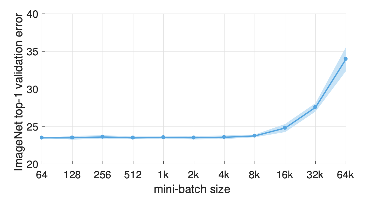
Figure 4-20. Large batch sizes have been shown to adversely affect the quality of the final trained model8.
Thus, setting the minibatch size in the context of distributed training is a complex optimization space of its own, as it affects both statistical accuracy (generalization) and hardware efficiency (utilization) of the model. Related work, focusing on this optimization, introduces a layerwise adaptive large batch optimization technique called LAMB, which has been able to reduce BERT training time from 3 days to just 76 minutes.
Minimizing I/O waits
GPUs and TPUs can process data much faster than CPUs, and when using distributed strategies with multiple accelerators, I/O pipelines can struggle to keep up, creating a bottleneck to more efficient training. Specifically, before a training step finishes, the data for the next step is not available for processing. This is shown in Figure 4-21. The CPU handles the input pipeline: reading data from storage, preprocessing, and sending to the accelerator for computation. As distributed strategies speed up training, more than ever it becomes necessary to have efficient input pipelines to fully utilize the computing power available.
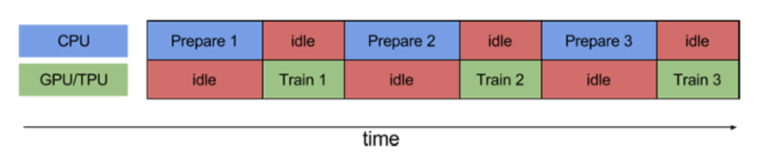
Figure 4-21. With distributed training on multiple GPU/TPUs available, it is necessary to have efficient input pipelines.
This can be achieved in a number of ways, including using optimized file formats like TFRecords and building data pipelines using the Tensorflow tf.data API. The tf.data API makes it possible to handle large amounts of data and has built in transformations useful for creating flexible, efficient pipelines. For example, tf.data.Dataset.prefetch overlaps the preprocessing and model execution of a training step so that while the model is executing training step N, the input pipeline is reading and preparing data for training step N + 1, as shown in Figure 4-22.
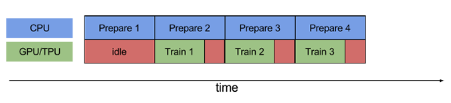
Figure 4-22. Prefetching overlaps preprocessing and model execution, so that while the model is executing one training step, the input pipeline is reading and preparing data for the next.
Design Pattern 15: Hyperparameter Tuning
In Hyperparameter Tuning, the training loop is itself inserted into an optimization method to find the optimal set of model hyperparameters.
Problem
In machine learning, model training involves finding the optimal set of breakpoints (in the case of decision trees), weights (in the case of neural networks), or support vectors (in the case of support vector machines). We term these model parameters. However, in order to carry out model training and find the optimal model parameters, we often have to hardcode a variety of things. For example, we might decide that the maximum depth of a tree will be 5 (in the case of decision trees), or that the activation function will be ReLU (for neural networks) or choose the set of kernels that we will employ (in SVMs). These parameters are called hyperparameters.
Model parameters refer to the weights and biases learned by your model. You do not have direct control over model parameters, since they are largely a function of your training data, model architecture, and many other factors. In other words, you cannot manually set model parameters. Your model’s weights are initialized with random values and then optimized by your model as it goes through training iterations. Hyperparameters, on the other hand, refer to any parameters that you, as a model builder, can control. They include values like learning rate, number of epochs, number of layers in your model, and more.
Manual Tuning
Because you can manually select the values for different hyperparameters, your first instinct might be a trial and error approach to finding the optimal combination of hyperparameter values. This might work for models that train in seconds or minutes, but it can quickly get expensive on larger models that require significant training time and infrastructure. Imagine you are training an image classification model that takes hours to train on GPUs. You settle on a few hyperparameter values to try and then wait for the results of the first training run. Based on these results you tweak the hyperparameters, train the model again, compare the results with the first run, and then settle on the best hyperparameter values by looking at the training run with the best metrics.
There are a few problems with this approach. First, you’ve spent nearly a day and many compute hours on this task. Second, there’s no way of knowing if you’ve arrived at the optimal combination of hyperparameter values. You’ve only tried two different combinations, and because you changed multiple values at once you don’t know which parameter had the biggest influence on performance. Even with additional trials, using this approach will quickly use up your time and compute resources and may not yield the most optimal hyperparameter values.
Note
We’re using the term trial here to refer to a single training run with a set of hyperparameter values.
Grid search and combinatorial explosion
A more structured version of the trial-and-error approach described earlier is known as grid search. When implementing hyperparameter tuning with grid search, we choose a list of possible values we’d like to try for each hyperparameter we want to optimize. For example, in Scikit-Learn’s RandomForestRegressor() model, let’s say we want to try the following combination of values for the model’s max_depth and n_estimators hyperparameters:
grid_values = {'max_depth': [5, 10, 100],'n_estimators': [100, 150, 200]}
Using grid search, we’d try every combination of the specified values, and then use the combination that yielded the best evaluation metric on our model. Let’s see how this works on a random forest model trained on the Boston housing dataset, which comes pre-installed with Scikit-learn. The model will predict the price of a house based on a number of factors. We can run grid search by creating an instance of the GridSearchCV class, and training the model passing it the values we defined earlier:
from sklearn.ensemble importRandomForestRegressorfrom sklearn.datasets import load_bostonX, y = load_boston(return_X_y=True)housing_model = RandomForestRegressor()grid_search_housing = GridSearchCV(housing_model, param_grid=grid_vals, scoring='max_error')grid_search_housing.fit(X, y)
Note that the scoring parameter here is the metric we want to optimize. In the case of this regression model, we want to use the combination of hyperparameters that results in the lowest error for our model. To get the best combination of values from the grid search, we can run grid_search_housing.best_params_. This returns the following:
{'max_depth': 100, 'n_estimators': 150}
We’d want to compare this to the error we’d get training a random forest regressor model without hyperparameter tuning, using Scikit-learn’s default values for these parameters. This grid search approach works okay on the small example we’ve defined above, but with more complex models we’d likely want to optimize more than two hyperparameters, each with a wide range of possible values. Eventually, grid search will lead to combinatorial explosion – as we add additional hyperparameters and values to our grid of options, the number of possible combinations we need to try and the time required to try them all increases significantly.
Another problem with this approach is that no logic is being applied when choosing different combinations. Grid search is essentially a brute force solution, trying every possible combination of values. Let’s say that after a certain max_depth value, our model’s error increases. The grid search algorithm doesn’t learn from previous trials, so it wouldn’t know to stop trying max_depth values after a certain threshold. It will simply try every value you provide no matter the results.
Note
Scikit-learn supports an alternative to grid search called RandomizedSearchCV which implements random search. Instead of trying every possible combination of hyperparameters from a set, you determine the number of times you’d like to randomly sample values for each hyperparameter. To implement random search in Scikit-learn, we’d create an instance of RandomizedSearchCV and pass it a dict similar to grid_values above, specifying ranges instead of specific values. Random search runs faster than grid search since it doesn’t try every combination in your set of possible values, but it is very likely that the optimal set of hyperparameters will not be among the ones randomly selected.
For robust hyperparameter tuning, we need a solution that scales, and learns from previous trials to find an optimal combination of hyperparameter values.
Solution
The keras-tuner library implements Bayesian optimization to do hyperparameter search directly in Keras. To use keras-tuner, we define our model inside a function that takes a hyperparameter argument, here called hp. We can then use hp throughout the function wherever we want to include a hyperparameter, specifying the hyperparameter’s name, data type, the value range we’d like to search, and how much to increment it each time we try a new one.
Instead of hardcoding the hyperparameter value when we define a layer in our Keras model, we define it using a hyperparameter variable. Here we want to tune the number of neurons in the first hidden layer of our neural network:
keras.layers.Dense(hp.Int('first_hidden', 32, 256, step=32), activation='relu')
first_hidden is the name we’ve given this hyperparameter, 32 is the minimum value we’ve defined for it, 256 is the maximum, and 32 is the amount we should increment this value by within the range we’ve defined. If we were building an MNIST classification model, the full function that we’d pass to keras-tuner might look like the following:
def build_model(hp):model = keras.Sequential([keras.layers.Flatten(input_shape=(28, 28)),keras.layers.Dense(hp.Int('first_hidden', 32, 256, step=32), activation='relu'),keras.layers.Dense(hp.Int('second_hidden', 32, 256, step=32), activation='relu'),keras.layers.Dense(10, activation='softmax')])model.compile(optimizer=tf.keras.optimizers.Adam(hp.Float('learning_rate', .005, .01, sampling='log')),loss='sparse_categorical_crossentropy',metrics=['accuracy'])return model
The keras-tuner library supports many different optimization algorithms. Here, we’ll instantiate our tuner with Bayesian optimization and optimize for validation accuracy:
import kerastuner as kttuner = kt.BayesianOptimization(build_model,objective='val_accuracy',max_trials=10)
The code to run the tuning job looks similar to training our model with fit(). As this runs, we’ll be able to see the values for the three hyperparameters that were selected for each trial. When the job completes, we can see the hyperparameter combination that resulted in the best trial. In Figure 4-23, we can see the example output for a single trial run using keras-tuner.
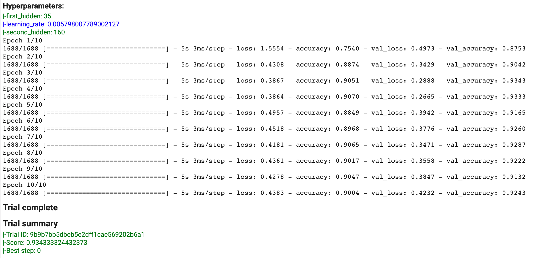
Figure 4-23. output for one trial run of hyperparameter tuning with keras-tuner. At the top we can see the hyperparameters selected by the tuner, and in the summary section we see the resulting optimization metric.
In addition to the examples shown here, there is additional functionality provided by keras-tuner that we haven’t covered. You can use it to experiment with different numbers of layers for your model by defining an hp.Int() parameter within a loop, and you can also provide a fixed set of values for a hyperparameter instead of a range. For more complex models, this hp.Choice() parameter could be used to experiment with different types of layers, like BasicLSTMCell and BasicRNNCell. keras-tuner runs in any environment where you can train a Keras model.
Why It Works
Although grid and random search are more efficient than a trial and error approach to hyperparameter tuning, they quickly become expensive for models requiring significant training time or having a large hyperparameter search space.
Since both machine learning models themselves and the process of hyperparameter search are optimization problems, it would follow that we would be able to use an approach that learns to find the optimal hyperparameter combination within a given range of possible values just like our models learn from training data.
We can think of hyperparameter tuning as an outer optimization loop (see Figure 4-24) where the inner loop consists of typical model training. Even though we depict neural networks as the model whose parameters are being optimized, this solution is applicable to other types of machine learning models.
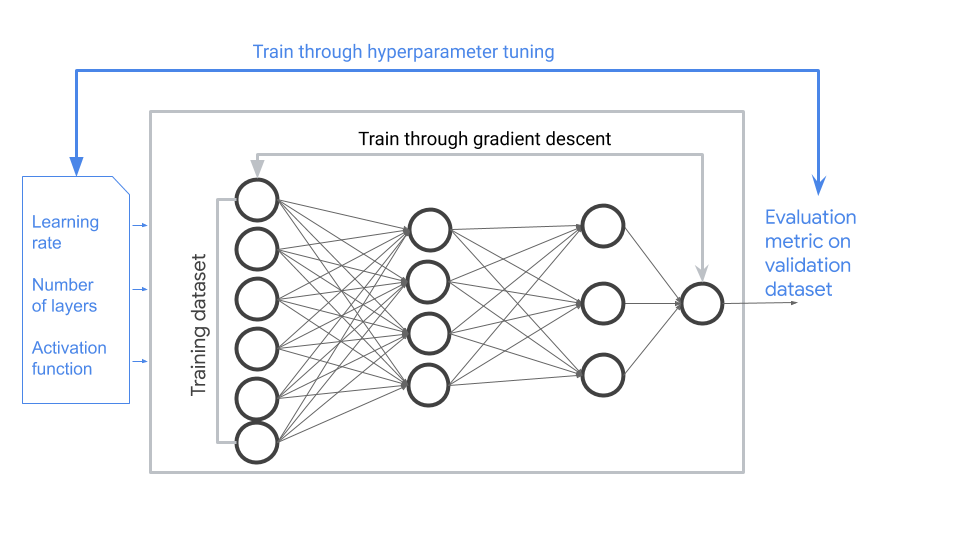
Figure 4-24. Hyperparameter tuning can be thought of as an outer optimization loop.
Non-linear optimization
The hyperparameters that need to be tuned fall into two groups: those related to model architecture and those related to model training. Model architecture hyperparameters, like the number of layers in your model or the number of neurons per layer, control the mathematical function that underlies the machine learning model. Parameters related to model training, like the number of epochs, learning rate, and batch size, control the training loop and often have to do with the way that the gradient descent optimizer works. Taking both these types of parameters into consideration, it is clear that the overall model function with respect to these hyperparameters is, in general, not differentiable.
The inner training loop is differentiable and the search for optimal parameters can be carried out through stochastic gradient descent. A single step of a machine learning model trained through stochastic gradient might take only a few milliseconds. On the other hand, a single trial in the hyperparameter tuning problem involves training a complete model on the training dataset and might take several hours. Moreover, the optimization problem for the hyperparameters will have to be solved through non-linear optimization methods that apply to non-differentiable problems.
Once we decide that we are going to use non-linear optimization methods, our choice of metric becomes wider. This metric will be evaluated on the validation dataset and does not have to be the same as the training loss. For a classification model, your optimization metric might be accuracy, and you’d therefore want to find the combination of hyperparameters that leads to the highest model accuracy even if the loss is binary cross entropy. For a regression model, you might want to optimize median absolute error even if the loss is squared error. In that case you’d want to find the hyperparameters that yield the lowest mean squared error. This metric can even be chosen based on business goals. For example, we might choose to maximize expected revenue or minimize losses due to fraud.
Bayesian optimization
Bayesian optimization is a technique for optimizing black-box functions, originally developed in the 1970s by Jonas Mockus. The technique has been applied to many domains, and was first applied to hyperparameter tuning in 2012. Here we’ll focus on Bayesian optimization as it relates to hyperparameter tuning. In this context, a machine learning model is our black-box function, since ML models produce a set of outputs from inputs we provide without requiring us to know the internal details of the model itself. The process of training our ML model is referred to as calling the objective function.
The goal of Bayesian optimization is to directly train our model as few times as possible since doing so is costly. Remember that each time we try a new combination of hyperparameters on our model, we need to run through our model’s entire training cycle. This might seem trivial with a small model like the Scikit-learn one we trained above, but for many production models the training process requires significant infrastructure and time.
Instead of training our model each time we try a new combination of hyperparameters, Bayesian optimization defines a new function that emulates our model but is much cheaper to run. This is referred to as the surrogate function – the inputs to this function are your hyperparameter values and the output is your optimization metric. The surrogate function is called much more frequently than the objective function, with the goal of finding an optimal combination of hyperparameters before completing a training run on your model. With this approach, more compute time is spent choosing the hyperparameters for each trial as compared with grid search. However, because this is significantly cheaper than running our objective function each time we try different hyperparameters, the Bayesian approach of using a surrogate function is preferred. Common approaches to generate the surrogate function include a Gaussian Process or a tree-structured Parzen estimator.
So far we’ve touched on the different pieces of Bayesian optimization, but how do they work together? First, we must choose the hyperparameters we want to optimize and define a range of values for each hyperparameter. This part of the process is manual, and will define the space in which our algorithm will search for optimal values. We’ll also need to define our objective function, which is the code that calls our model training process. From there, Bayesian optimization develops a surrogate function to simulate our model training process and uses that function to determine the best combination of hyperparameters to run on our model. It is only once this surrogate arrives at what it thinks is a good combination of hyperparameters that we do a full training run (trial) on our model. The results of this are then fed back to the surrogate function and the process is repeated for the number of trials we’ve specified.
Tradeoffs and Alternatives
Genetic algorithms are an alternative to Bayesian methods for hyperparameter tuning, but they tend to require many more model training runs than Bayesian methods. We’ll also show you how to use a managed service for hyperparameter tuning optimization on models built with a variety of ML frameworks.
Fully managed hyperparameter tuning
The keras-tuner approach may not scale to large machine learning problems because we’d like the trials to happen in parallel, and the likelihood of machine error and other failure increases as the time for model training stretches into the hours. Hence, a fully-managed, resilient approach that provides black-box optimization is useful for hyperparameter tuning. An example of a managed service that implements Bayesian optimization is the hyperparameter tuning service provided by Google Cloud AI Platform. This service is based on Vizier, the black-box optimization tool used internally at Google.
The underlying concepts of the Cloud service work similarly to keras-tuner: you specify each hyperparameter’s name, type, range, and scale, and these values are referenced in your model training code. We’ll show you how to run hyperparameter tuning in AI Platform using a PyTorch model trained on the BigQuery natality dataset to predict a baby’s birth weight.
The first step is to create a config.yaml file specifying the hyperparameters you want the job to optimize, along with some other metadata on your job. One benefit of using the Cloud service is that you can scale your tuning job by running it on GPUs or TPUs and spreading it across multiple parameter servers. In this config file, you also specify the total number of hyperparameter trials you want to run and how many of these trials you want to run in parallel. The more you run in parallel, the faster your job will run. However, the benefit of running fewer trials in parallel is that the service will be able to learn from the results of each completed trial to optimize the next ones.
For our model, a sample config file that makes use of GPUs might look like the following. In this example, we’ll tune three hyperparameters – our model’s learning rate, the optimizer’s momentum value, and the number of neurons in our model’s hidden layer. We also specify our optimization metric. In this example our goal will be to minimize our model’s loss on our validation set:
trainingInput:scaleTier: BASIC_GPUparameterServerType: large_modelworkerCount: 9parameterServerCount: 3hyperparameters:goal: MINIMIZEmaxTrials: 10maxParallelTrials: 5hyperparameterMetricTag: val_errorenableTrialEarlyStopping: TRUEparams:- parameterName: lrtype: DOUBLEminValue: 0.0001maxValue: 0.1scaleType: UNIT_LINEAR_SCALE- parameterName: momentumtype: DOUBLEminValue: 0.0maxValue: 1.0scaleType: UNIT_LINEAR_SCALE- parameterName: hidden-layer-sizetype: INTEGERminValue: 8maxValue: 32scaleType: UNIT_LINEAR_SCALE
Note
Instead of using a config file to define these values, you can also do this using the AI Platform Python API.
In order to do this, we’ll need to add an argument parser to our code that will specify the arguments we defined in the file above, and then refer to these hyperparameters where they appear throughout our model code.
Next, we’ll build our model using PyTorch’s nn.Sequential API with the SGD optimizer. Since our model predicts baby weight as a float, this will be a regression model. We specify each of our hyperparameters using the args variable, which contains the variables defined in our argument parser:
import torch.nn asnnmodel = nn.Sequential(nn.Linear(num_features, args.hidden_layer_size),nn.ReLU(),nn.Linear(args.hidden_layer_size, 1))optimizer = torch.optim.SGD(model.parameters(), lr=args.lr, momentum=args.momentum)
At the end of our model training code we’ll create an instance of HyperTune(), and tell it the metric we’re trying to optimize. This will report the resulting value of our optimization metric after each training run. It’s important that whichever optimization metric we choose is calculated on our test or validation datasets, and not our training dataset:
import hypertunehpt = hypertune.HyperTune()val_mse = 0num_batches = 0criterion = nn.MSELoss()with torch.no_grad():for i, (data, label)in enumerate(validation_dataloader):num_batches += 1y_pred = model(data)mse = criterion(y_pred, label.view(-1,1))val_mse += mse.item()avg_val_mse = (val_mse / num_batches)hpt.report_hyperparameter_tuning_metric(hyperparameter_metric_tag='val_mse',metric_value=avg_val_mse,global_step=epochs)
Once we’ve submitted our training job to AI Platform we can monitor logs in the Cloud console. After each trial completes, you’ll be able to see the values chosen for each hyperparameter and the resulting value of your optimization metric, as seen in Figure 4-25.
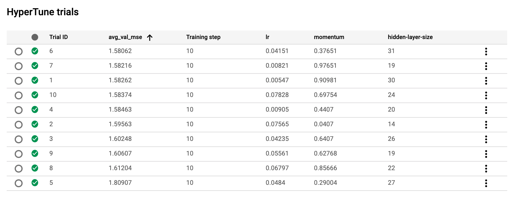
Figure 4-25. A sample of the HyperTune summary in the AI Platform console. This is for a PyTorch model optimizing 3 model parameters, with the goal of minimizing mean squared error on the validation dataset.
By default, AI Platform Training will use Bayesian optimization for your tuning job, but you can also specify if you’d like to use grid or random search algorithms instead. The Cloud service also optimizes your hyperparameter search across training jobs. If we run another training job similar to the one above, but with a few tweaks to our hyperparameters and search space, it’ll use the results of our last job to efficiently choose values for the next set of trials.
We’ve shown a PyTorch example here, but you can use AI Platform Training for hyperparameter tuning in any machine learning framework by packaging your training code and providing a setup.py file that installs any library dependencies.
Genetic algorithms
We’ve explored various algorithms for hyperparameter optimization: manual search, grid search, random search, and Bayesian optimization. Another less common alternative is a genetic algorithm, which is roughly based on Charles Darwin’s evolutionary theory of natural selection. This theory, also known as “survival of the fittest,” posits that the highest performing (“fittest”) members of a population will survive and pass their genes to future generations, while less fit members will not. Genetic algorithms have been applied to different types of optimization problems, including hyperparameter tuning.
As it relates to hyperparameter search, a genetic approach works by first defining a fitness function. This function measures the quality of a particular trial, and can typically be defined by your model’s optimization metric (accuracy, error, and so on). After defining your fitness function, you randomly select a few combinations of hyperparameters from your search space and run a trial for each of those combinations. You then take the hyperparameters from the trials that performed best, and use those values to define your new search space. This search space becomes your new “population” and you use it to generate new combinations of values to use in your next set of trials. You would continue this process, narrowing down the number of trials you run until you’ve arrived at a result that satisfies your requirements.
Because they use the results of previous trials to improve, genetic algorithms are “smarter” than manual, grid, and random search. However, when the hyperparameter search space is large, the complexity of genetic algorithms increases. Rather than using a surrogate function as a proxy for model training like in Bayesian optimization, genetic algorithms require training your model for each possible combination of hyperparameter values. Additionally, at the time of writing, genetic algorithms are less common and there are fewer ML frameworks that support it out of the box for hyperparameter tuning.
Summary
This chapter focused on design patterns that modify the typical SGD training loop of machine learning. We started with looking at the Useful Overfitting pattern, which covered situations where overfitting is beneficial. For example, when using data driven methods like machine learning to approximate solutions to complex dynamical systems or PDEs where the full input space can be covered, overfitting on the training set is the goal. Overfitting is also useful as a technique when developing and debugging ML model architectures. Next we covered model Checkpoints and how to use them when training ML models. In this design pattern, we save the full state of the model periodically during training. These checkpoints can be used as the final model, as in the case of early stopping, or be used as the starting points in the case of training failures or fine tuning.
The Transfer Learning design pattern covered reusing parts of a previously trained model. Transfer learning is a useful way to leverage the learned feature extraction layers of the pre-trained model when your own dataset is limited. It can also be used to fine-tune a pre-trained model that was trained on a large generic dataset to your more specialized dataset. We then discussed the Distribution Strategy design pattern. Training large complex neural networks can take a considerable amount of time. Distribution strategies offer various ways in which the training loop can be modified to be carried out at scale over multiple workers, using parallelization and hardware accelerators.
Lastly, the Hyperparameter Tuning design pattern discussed how the SGD training loop itself can be optimized with respect to model hyperparameters. We saw some useful libraries that can be used to implement hyperparameter tuning for models created with Keras and PyTorch.
The next chapter looks at design patterns related to resilience (to large numbers of requests, spiky traffic, or change management) when placing models into production.
1 It may, of course, not be the case that we can learn the network using gradient descent just because there exists such a neural network (this is why changing the model architecture by adding layers helps – it makes the loss landscape more amenable to SGD).
2 J. Deng, W. Dong, R. Socher, L.-J. Li, K. Li and L. Fei-Fei, ImageNet: A Large-Scale Hierarchical Image Database. IEEE Computer Vision and Pattern Recognition (CVPR), 2009 http://www.image-net.org/papers/imagenet_cvpr09.pdf
3 Progressive fine-tuning was introduced in a paper by Wang and Zhang
4 For more information, see this article.
5 V. Campos et. al., “Distributed training strategies for a computer vision deep learning algorithm on a distributed GPU cluster”, International Conference on Computational Science, ICCS 2017, 12-14 June 2017.
6 V. Campos et. al., “Distributed training strategies for a computer vision deep learning algorithm on a distributed GPU cluster”, International Conference on Computational Science, ICCS 2017, 12-14 June 2017.
7 Jeffrey Dean, et al. “Large Scale Distributed Deep Networks”, NIPS Proceedings, 2012.
8 P. Goyal, et al., “Accurate, Large Minibatch SGD: Training ImageNet in 1 Hour”, 2017.