
Chapter 5. Design Patterns for Resilient Serving
The purpose of a machine learning model is to use it to make inferences on data it hasn’t seen during training. Therefore, once a model has been trained, it is typically deployed into a production environment and used to make predictions in response to incoming requests. Software that is deployed into production environments is expected to be resilient and require little in the way of human intervention to keep it running. The design patterns in this chapter solve problems associated with resilience under different circumstances, as it relates to production ML models.
The Stateless Serving Function design pattern allows the serving infrastructure to scale and handle thousands or even millions of prediction requests per second. The Batch Serving design pattern allows the serving infrastructure to asynchronously handle occasional or periodic requests for millions to billions of predictions. These patterns are useful beyond resilience in that they reduce coupling between creators and users of machine learning models.
The Continued Model Evaluation design pattern handles the common problem of detecting when a deployed model is no longer fit-for-purpose. The Two Phased Prediction design pattern provides a way to address the problem of keeping models sophisticated and performant when they have to be deployed onto distributed devices. The Keyed Predictions design pattern is a necessity to scalably implement several of the design patterns discussed in this chapter.
Design pattern 16: Stateless Serving Function
The Stateless Serving Function design pattern makes it possible for a production ML system to synchronously handle thousands to millions of prediction requests per second. The production ML system is designed around a stateless function that captures the architecture and weights of a trained model.
Problem
Let’s take a text classification model that uses, as its training data, movie reviews from the Internet Movie Database (IMDb). For the initial layer of the model, we will use a pre-trained embedding that maps text to 20-dimensional embedding vectors (for full code, see the serving_function.ipynb notebook in the GitHub repository for this book):
model = tf.keras.Sequential()
embedding = (
        "https://tfhub.dev/google/tf2-preview/gnews-swivel-20dim-with-oov/1")
hub_layer = hub.KerasLayer(embedding, input_shape=[],
                           dtype=tf.string, trainable=True, name='full_text')
model.add(hub_layer)
model.add(tf.keras.layers.Dense(16, activation='relu', name='h1_dense'))
model.add(tf.keras.layers.Dense(1, name='positive_review_logits'))
The embedding layer is obtained from TensorFlow Hub and marked as being trainable, so that we can carry out Fine Tuning (see the Transfer Learning section in Chapter 4) on the vocabulary found in IMDB reviews. The subsequent layers are that of a simple neural network with one hidden layer and an output logits layer. This model can then be trained on the dataset of movie reviews to learn to predict whether or not a review is positive or negative.
Once the model has been trained, we can use it to carry out inferences on how positive a review is:
review1 = 'The film is based on a prize-winning novel.'
review2 = 'The film is fast moving and has several great action scenes.'
review3 = 'The film was very boring. I walked out half-way.'
logits = model.predict(x=tf.constant([review1, review2, review3]))
The result is a 2D array, that might be something like:
[[ 0.6965847]
 [ 1.61773  ]
 [-0.7543597]]
There are several problems with carrying out inferences by calling model.predict() on an in-memory object (or a trainable object loaded into memory) as described above:
-
We have to load the entire Keras model into memory. The text embedding layer, which was set up to be trainable, can be quite large because it needs to store embeddings for the full vocabulary of English words. Deep learning models with many layers can also be quite large.
-
The above architecture imposes limits on the latency that can be achieved because calls to the predict() method have to be sent one-by-one.
-
Even though the data scientist’s programming language of choice is Python, model inference is likely to be invoked by programs written by developers who prefer other languages, or on mobile platforms like Android or iOS which require different languages
-
The model input and output that is most effective for training may not be user-friendly. In our example, the model output was logits because it is better for gradient descent. This is why the second number in the output array is greater than 1. What clients will typically want is the sigmoid of this, so that the output range is 0–1 and can be interpreted in a more user-friendly format as a probability. We will want to carry out this post-processing on the server, so that the client code is as simple as possible. Similarly, the model may have been trained from compressed, binary records, whereas during production, we might want to be able to handle self-descriptive input formats like JSON.
Solution
The solution consists of the following steps:
-
Export the model into a format that captures the mathematical core of the model and programming language agnostic.
-
In the production system, the formula consisting of the “forward” calculations of the model is restored as a stateless function.
-
The stateless function is deployed into a framework that provides a REST endpoint.
Model export
The first step of the solution is to export the model into a format (TensorFlow uses SavedModel, but ONNX is another choice) that captures the mathematical core of the model. The entire model state (learning rate, dropout, short-circuit, etc.) doesn’t need to be saved – just the mathematical formula required to compute the output from the inputs. Typically, the trained weight values are constants in the mathematical formula.
In Keras, this is accomplished by:
model.save('export/mymodel')
The SavedModel format relies on protocol buffers for a platform-neutral, efficient restoration mechanism. In other words, the model.save() method writes the model as a protocol buffer (with the extension .pb) and externalizes the trained weights, vocabularies, and so on into other files in a standard directory structure:
export/.../variables/variables.data-00000-of-00001
export/.../assets/tokens.txt
export/.../saved_model.pb
Inference in Python
In a production system, the model’s formula is restored from the protocol buffer and other associated files as a stateless function that conforms to a specific model signature with input and output variable names and data types.
We can use the TensorFlow saved_model_cli tool to examine the exported files to determine the signature of the stateless function that we can use in serving:
saved_model_cli show --dir ${export_path}
     --tag_set serve --signature_def serving_default
This outputs:
The given SavedModel SignatureDef contains the following input(s):inputs['full_text_input'] tensor_info:dtype: DT_STRINGshape: (-1)name: serving_default_full_text_input:0The given SavedModel SignatureDef contains the following output(s):outputs['positive_review_logits'] tensor_info:dtype: DT_FLOATshape: (-1, 1)name: StatefulPartitionedCall_2:0Method name is: tensorflow/serving/predict
The signature specifies that the prediction method takes a one-element array as input (called full_text_input) that is a string, and outputs one floating point number whose name is positive_review_logits. These names come from the names that we assigned to the Keras layers:
hub_layer = hub.KerasLayer(..., name='full_text')...model.add(tf.keras.layers.Dense(1, name='positive_review_logits'))
Here is how we can obtain the serving function and use it for inference:
serving_fn = tf.keras.models.load_model(export_path).signatures['serving_default']outputs = serving_fn(full_text_input=tf.constant([review1, review2, review3]))logit = outputs['positive_review_logits']
Note how we are using the input and output names from the serving function in the code.
Create web endpoint
The code above can be put into a web application or serverless framework such as Google App Engine, Heroku, AWS Lambda, Azure Functions, Google Cloud Functions, Cloud Run, and so on. What all these frameworks have in common is that they allow the developer to specify a function that needs to be executed. The frameworks take care of autoscaling the infrastructure so as to handle large numbers of prediction requests per second at low-latency.
For example, we can invoke the serving function from within Cloud Functions as follows:
serving_fn = Nonedef handler(request):global serving_fnif serving_fn is None:serving_fn = (tf.keras.models.load_model(export_path).signatures['serving_default'])request_json = request.get_json(silent=True)if request_json and 'review' in request_json:review = request_json['review']outputs = serving_fn(full_text_input=tf.constant([review]))return outputs['positive_review_logits']
Note that we should be careful to define the serving function as a global variable (or a singleton class) so that it isn’t reloaded in response to every request. In practice, the serving function will be reloaded from the export path (on Google Cloud Storage) only in the case of cold starts.
Why It Works
The approach of exporting a model to a stateless function, and deploying the stateless function in a web application framework works because web application frameworks offer autoscaling, can be fully managed, and are language-neutral. They are also familiar to software and business development teams who may not have experience with machine learning. This also has benefits for agile development – ML engineer or data scientist can independently change the model and all the application developer needs to do is change the endpoint they are accessing.
Autoscaling
Scaling web endpoints to millions of requests per second is a well-understood engineering problem. Rather than build services unique to machine learning, we can rely on the decades of engineering work that has gone into building resilient web applications and web servers. Cloud providers know how to autoscale web endpoints efficiently, and with minimal warm-up times.
We don’t even need to write the serving system ourselves. Most modern enterprise machine learning frameworks come with a serving subsystem. For example, TensorFlow provides TensorFlow Serving and PyTorch provides TorchServe. If we use these serving subsystems, we can simply provide the exported file and the software takes care of creating a web endpoint.
Fully managed
Cloud platforms abstract away the managing and installation of components like TensorFlow Serving as well. Thus, on Google Cloud, deploying the serving function as a REST API is as simple as running this command-line program providing the location of the SavedModel output:
gcloud ai-platform versions create ${MODEL_VERSION}
       --model ${MODEL_NAME} --origin ${MODEL_LOCATION}
       --runtime-version $TFVERSION
In Amazon’s Sagemaker, deployment of a TensorFlow SavedModel is similarly simple, and achieved using:
model = Model(model_data=MODEL_LOCATION, role='SomeRole')
predictor = model.deploy(initial_instance_count=1,
                         instance_type='ml.c5.xlarge')
With a REST endpoint in place, we can send in JSON of the form:
{"instances":
  [
      {"reviews": "The film is based on a prize-winning novel."},
      {"reviews": "The film is fast moving and has several great action scenes."},
      {"reviews": "The film was very boring. I walked out half-way."}
  ]
}
and get back the predicted values also wrapped in a JSON structure.
{"predictions": [{ "positive_review_logits": [0.6965846419334412]}, {"positive_review_logits": [1.6177300214767456]}, {"positive_review_logits": [-0.754359781742096]}]}
Note
TIP
By allowing clients to send JSON requests with multiple instances in the request, called batching, we are allowing clients to trade off the higher throughput associated with fewer network calls against the increased parallelization if they send more requests with fewer instances per request.
Besides batching, there are other knobs and levers to improve performance or lower cost. Using a machine with more powerful GPUs, for example, typically helps to improve the performance of deep learning models. Choosing a machine with multiple accelerators and/or threads helps improve the number of requests per second. Using an autoscaling cluster of machines can help lower cost on spiky workloads. These kinds of tweaks are often done by the ML/DevOps team; some are ML-specific, some are not.
Language-neutral
Every modern programming language can speak REST, and a discovery service is provided to auto generate the necessary HTTP stubs. Thus, Python clients can invoke the REST API as follows. Note that there is nothing framework specific in the code below. Because the cloud service abstracts the specifics of our ML model, we don’t need to provide any references to Keras or TensorFlow):
credentials = GoogleCredentials.get_application_default()
api = discovery.build("ml", "v1", credentials = credentials,
            discoveryServiceUrl = "https://storage.googleapis.com/cloud-ml/discovery/ml_v1_discovery.json")
request_data = {"instances":
  [
      {"reviews": "The film is based on a prize-winning novel."},
      {"reviews": "The film is fast moving and has several great action scenes."},
      {"reviews": "The film was very boring. I walked out half-way."}
  ]
}
parent = "projects/{}/models/imdb".format("PROJECT", "v1")
response = api.projects().predict(body = request_data,
                                  name = parent).execute()
The equivalent of the above code can be written in many languages (we show Python because we assume you are somewhat familiar with it). At the time that this book is being written, developers can access the Discovery API from Java, PHP, .NET, JavaScript, Objective-C, Dart, Ruby, Node.js, and Go.
Powerful ecosystem
Because web application frameworks are so widely used, there is a lot of tooling available to measure, monitor, and manage web applications. If we deploy the ML model to a web application framework, the model can be monitored and throttled using tools that Software Reliability Engineers (SREs), IT administrators and DevOps personnel are familiar with. They do not have to know anything about machine learning.
Similarly, your business development colleagues know how to meter and monetize web applications using API gateways. They can carry over that knowledge and apply it to metering and monetizing machine learning models.
Tradeoffs and Alternatives
As the joke by David Wheeler goes, the solution to any problem in computer science is to add an extra level of indirection. Introduction of an exported stateless function specification provides that extra level of indirection. The Stateless Serving Function design pattern allows us to change the serving signature to provide extra functionality, like additional pre- and post-processing, beyond what the ML model does. In fact, it is possible to use this design pattern to provide multiple endpoints for a model. This design pattern can also help with creating low-latency, online prediction for models that are trained on systems, such as data warehouses, that are typically associated with long-running queries.
Custom serving function
The output layer of our text classification model is a dense layer whose output is in the range (-∞,∞):
model.add(tf.keras.layers.Dense(1, name='positive_review_logits'))
Our loss functions takes this into account:
model.compile(optimizer='adam',
              loss=tf.keras.losses.BinaryCrossentropy(
                      from_logits=True),
              metrics=['accuracy'])
When we use the model for prediction, the model naturally returns what it was trained to predict, and outputs the logits. What clients expect, however, is the probability that the review is positive. To solve this, we need to return the sigmoid output of the model.
We can do this by writing a custom serving function and exporting it instead. Here is a custom serving function in Keras that adds a probability and returns a dictionary that contains both the logits and the probabilities for each of the reviews provided as input:
@tf.function(input_signature=[tf.TensorSpec([None],
                              dtype=tf.string)])def add_prob(reviews):
    logits = model(reviews, training=False) # call model
    probs = tf.sigmoid(logits)
    return {
        'positive_review_logits' : logits,
        'positive_review_probability' : probs
    }
We can then export the above function as the serving default:
model.save(export_path,
           signatures={'serving_default': add_prob})
The add_prob method definition is saved in the export_path, and will be invoked in response to a client request.
The serving signature of the exported model reflects the new input name (note the name of the input parameter to add_prob) and the output dictionary keys and data types:
The given SavedModel SignatureDef contains the following input(s):inputs['reviews'] tensor_info:dtype: DT_STRINGshape: (-1)name: serving_default_reviews:0The given SavedModel SignatureDef contains the following output(s):outputs['positive_review_logits'] tensor_info:dtype: DT_FLOATshape: (-1, 1)name: StatefulPartitionedCall_2:0outputs['positive_review_probability'] tensor_info:dtype: DT_FLOATshape: (-1, 1)name: StatefulPartitionedCall_2:1Method name is: tensorflow/serving/predict
When this model is deployed and used for inference, the output JSON contains both the logits and the probability:
{'predictions': [{'positive_review_probability': [0.6674301028251648], 'positive_review_logits': [0.6965846419334412]}, {'positive_review_probability': [0.8344818353652954], 'positive_review_logits': [1.6177300214767456]}, {'positive_review_probability': [0.31987208127975464], 'positive_review_logits': [-0.754359781742096]}]}
Note that the add_prob is a function that we write. In this case, we did a bit of postprocessing of the output. However, we could have done pretty much any (stateless) thing that we want inside that function.
Multiple signatures
It is quite common for models to support multiple objectives or clients who have different needs. While outputting a dictionary can allow different clients to pull out whatever they want, this may not be ideal in some cases. For example, the function we had to invoke to get a probability from the logits was simply tf.sigmoid(). This is pretty inexpensive, and there is no problem with computing it even for clients who will discard it. On the other hand, if the function had been expensive, computing it for clients who don’t need the value can add considerable overhead.
If a small number of clients require a very expensive operation, it is helpful to provide multiple serving signatures and have the client inform the serving framework which signature to invoke. This is done by specifying a name other than serving_default when the model is exported. For example, we might write out two signatures using:
model.save(export_path, signatures={
        'serving_default': func1,
        'expensive_result': func2,
   })
Then, the input JSON request includes the signature name to choose which serving endpoint of the model is desired:
{
  "signature_name": "expensive_result",
   {"instances": …}
}
Online prediction
Because the exported serving function is ultimately just a file format, it can be used to provide online prediction capabilities when the original machine learning training framework does not natively support online predictions.
For example, we can train a model to infer whether or not a baby will require attention by training a logistic regression model on the natality dataset:
CREATE OR REPLACE MODEL mlpatterns.neutral_3classes
OPTIONS(model_type='logistic_reg', input_label_cols=['health']) AS
SELECT
  IF(apgar_1min = 10, 'Healthy', IF(apgar_1min >= 8, 'Neutral', 'NeedsAttention')) AS health,
  plurality,
  mother_age,
  gestation_weeks,
  ever_born
FROM `bigquery-public-data.samples.natality`
WHERE apgar_1min <= 10
Once the model is trained, we can carry out prediction using SQL:
SELECT * FROM ML.PREDICT(MODEL mlpatterns.neutral_3classes,
    (SELECT
     2 AS plurality,
     32 AS mother_age,
     41 AS gestation_weeks,
     1 AS ever_born
    )
)
However, BigQuery is primarily for distributed data processing. While it was great for training the ML model on gigabytes of data, using such a system to carry out inference on a single row is not the best fit – latencies can be as high as a second or two. Rather, the ML.PREDICT functionality is more appropriate for Batch Serving.
In order to carry out online prediction, we can ask BigQuery to export the model as a TensorFlow SavedModel:
bq extract -m --destination_format=ML_TF_SAVED_MODELmlpatterns.neutral_3classes gs://${BUCKET}/export/baby_health
Now, we can deploy the SavedModel into a serving framework like Cloud AI Platform that supports SavedModel to get the benefits of low-latency, autoscaled ML model serving. See the notebook in GitHub for the complete code.
Even if this ability to export the model as a SavedModel did not exist, we could have extracted the weights, written a mathematical model to carry out the linear model, containerized it and deployed the container image into a serving platform.
Prediction Library
Instead of deploying the Serving Function as a microservice that can be invoked via a REST API, it is possible to implement the prediction code as a library function. The library function would load the exported model the first time it is called, invoke model.predict() with the provided input, and return the result. Application developers that need to predict with the library can then include the library with their applications.
A library function is a better alternative than a microservice if the model can not be called over a network either because of physical reasons (there is no network connectivity) or because of performance constraints. The library function approach also places the computational burden on the client, and this might be preferable from a budgetary standpoint. Using the library approach with TensorFlow.js can avoid cross-site problems when there is a desire to have the model running in a browser.
The main drawback of the library approach is that maintenance and updates of the model are difficult – all the client code that uses the model will have to be updated to use the new version of the library. The more commonly a model is updated, the more attractive a microservices approach becomes. A secondary drawback is that the library approach is restricted to programming languages for which libraries are written whereas the REST API approach opens up the model to applications written in pretty much any modern programming language.
The library developer should take care to employ a threadpool and use parallelization to support the necessary throughput. However, there is usually a limit to the scalability achievable with this approach.
Design pattern 17: Batch Serving
Batch serving uses software infrastructure commonly used for distributed data processing to carry out inference on a large number of instances all at once.
Problem
Commonly, predictions are carried one at a time and on demand. Whether or not a credit card transaction is fraudulent is determined at the time a payment is being processed. Whether or not a baby requires intensive care is determined when the baby is examined immediately after birth. Therefore, when you deploy a model into a ML serving framework, it is set up to process one instance, or at most a few thousands of instances, embedded in a single request.
The serving framework is architected to process an individual request synchronously and as quickly as possible, as discussed in the Stateless Serving Function design pattern. The serving infrastructure is usually designed as a microservice that offloads the heavy computation (such as with deep convolutional neural networks) to high-performance hardware such as Tensor Processing Units (TPUs) or Graphics Processing Units (GPUs) and minimizes the inefficiency associated with multiple software layers.
However, there are circumstances where predictions need to be carried out asynchronously over large volumes of data. For example, determining whether to reorder a stock keeping unit (SKU) might be an operation that is carried out hourly, not every time the SKU is bought at the cash register. Music services might create personalized daily playlists for every one of their users and push it out to those users. The personalized playlist is not created on-demand in response to every interaction that the user makes with the music software. Because of this, the ML model needs to make predictions for millions of instances at a time, not one instance at a time.
Attempting to take a software endpoint that is designed to handle one request at a time and sending it millions of SKUs or billions of users will overwhelm the ML model.
Solution
The Batch Serving design pattern uses distributed data processing infrastructure (MapReduce, Apache Spark, BigQuery, Apache Beam, and so on) to carry out ML inference on a large number of instances asynchronously.
In the discussion on the Stateless Serving Function design pattern, we trained a text classification model to output whether a review was positive or negative. Let’s say that we want to apply this model to every complaint that has ever been made to the United States’ Consumer Finance Protection Bureau (CFPB).
We can load the Keras model into BigQuery as follows (complete code is available in a notebook in GitHub):
CREATE OR REPLACE MODEL mlpatterns.imdb_sentimentOPTIONS(model_type='tensorflow', model_path='gs://.../*')
Where normally, one would train a model using data in BigQuery, here we are simply loading an externally trained model. Having done that, though, it is possible to use BigQuery to carry out ML predictions. For example, this SQL query:
SELECT * FROMML.PREDICT(MODEL mlpatterns.imdb_sentiment,(SELECT 'This was very well done.' AS reviews) )
returns a positive_review_probability of 0.82.
Using a distributed data processing system like BigQuery to carry out one-off predictions is not very efficient. However, what if we want to apply the machine learning model to every complaint in the CFPB database?1 We can simply adapt the query above, making sure to alias the consumer_complaint_narrative column in the column as the reviews to be assessed:
SELECT * FROM ML.PREDICT(MODEL mlpatterns.imdb_sentiment,(SELECT consumer_complaint_narrative AS reviewsFROM `bigquery-public-data`.cfpb_complaints.complaint_database WHERE consumer_complaint_narrative IS NOT NULL ) )
The database has more than 1.5 million complaints, but they get processed in about 30 seconds, proving the benefits of using a distributed data processing framework.
Why It Works
The Stateless Serving Function design pattern is set up for low-latency serving to support thousands of simultaneous queries. Using such a framework for occasional or periodic processing of millions of items can get quite expensive. If these requests are not latency-sensitive, it is more cost effective to use a distributed data processing architecture to invoke machine learning models on millions of items. The reason is that invoking an ML model on millions of items is an embarrassingly parallel problem – it is possible to take the million items, break it down into 1000 groups of 1000 items each, send each group of items to a machine, and then combine the results. The result of the machine learning model on item #2000 is completely independent of the result of the machine learning model on item #3000, and so it is possible to divide up the work and conquer it.
Take, for example, the query to find the 5 most positive complaints:
WITH all_complaints AS (
SELECT * FROM ML.PREDICT(MODEL mlpatterns.imdb_sentiment,
  (SELECT consumer_complaint_narrative AS reviews
   FROM `bigquery-public-data`.cfpb_complaints.complaint_database
   WHERE consumer_complaint_narrative IS NOT NULL
   )
)
)
SELECT * FROM all_complaints
ORDER BY positive_review_probability DESC LIMIT 5
Looking at the execution details in the BigQuery web console, we see that the entire query took 35 seconds (see the box marked #1 in Figure 5-1).
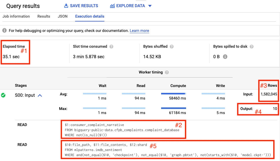
Figure 5-1. The first two steps of a query to find the 5 most “positive” complaints in the Consumer Finance Protection Bureau dataset of consumer complaints.
The first step (see box #2 in Figure 5-1) reads the consumer_complaint_narrative column from the BigQuery public dataset where the complaint narrative is not NULL. From the number of rows highlighted in box #3, we learn that this involves reading 1,582,045 values. The output of this step is written into 10 shards (see box #4 of Figure 5-1).
The second step reads the data from this shard (note the $12:shard in the query), but also obtains the file_path and file_contents of the machine learning model imdb_sentiment and applies the model to the data in each shard. The way MapReduce works is that each shard is processed by a worker, so the fact that there are 10 shards indicates that the second step is being done by 10 workers. The original 1.5 millions rows would have been stored over many files, and so the first step was likely to have been processed by as many workers as the number of files that comprised that dataset.
The remaining steps are shown in Figure 5-2.
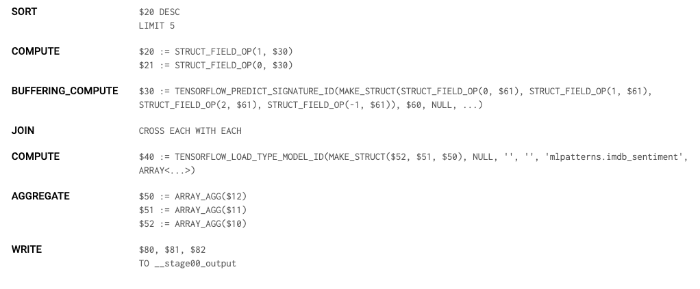
Figure 5-2. Third, and subsequent steps, of the query to find the 5 most “positive” complaints.
The third step sorts the dataset in descending order and takes 5. This is done on each worker, so each of the 10 workers finds the 5 most positive complaints in “their” shard. The remaining steps retrieve and format the remaining bits of data and write it to the output.
The final step (not shown) takes the 50 complaints, sorts them, and selects the 5 that form the actual result. The ability to separate work in this work across many workers is what enables BigQuery to carry out the entire operation on 1.5 million complaint documents in 35 seconds.
Tradeoffs and Alternatives
The Batch Serving design pattern depends on the ability to split a task across multiple workers. So, it is not restricted to data warehouses or even to SQL. Any MapReduce framework will work. However, SQL data warehouses tend to be the easiest and are often the default choice especially when the data is structured in nature.
Even though Batch Serving is used when latency is not a concern, it is possible to incorporate precomputed results and periodic refreshing to use this in scenarios where the space of possible prediction inputs is limited.
Batch and stream pipelines
Frameworks like Apache Spark or Apache Beam are useful when the input needs preprocessing before it can be supplied to the model, if the machine learning model outputs require postprocessing, or if either the preprocessing or postprocessing are hard to express in SQL. If the inputs to the model are images, audio, or video, then SQL is not an option and it is necessary to use a data processing framework that can handle unstructured data. These frameworks can also take advantage of accelerated hardware like TPUs and GPUs to carry out preprocessing of the images.
Another reason to use a framework like Apache Beam is if the client code needs to maintain state. A common reason that the client needs to maintain state is if one of the inputs to the ML model is a time-windowed average. In that case, the client code has to carry out moving averages of the incoming stream of data and supply the moving average to the ML model.
Imagine that we are building a comment moderation system and we wish to reject people who comment more than two times a day about a specific person. For example, the first two times that a commenter writes something about President Obama, we will let it go, but block all attempts by that commenter to mention President Obama for the rest of the day. This is an example of postprocessing that needs to maintain state because we need a counter of the number of times that each commenter has mentioned a particular celebrity. Moreover, this counter needs to be over a rotating time period of 24 hours.
We can do this using a distributed data processing framework that can maintain state. Enter Apache Beam. Invoking an ML model to identify mentions of a celebrity and tying them to a canonical knowledge graph (so that a mention of Obama and a mention of President Obama both tie to en.wikipedia.org/wiki/Barack_Obama) from Apache Beam can be accomplished using (see this notebook in GitHub for complete code):
 | beam.Map(lambda x : nlp.Document(x, type='PLAIN_TEXT'))
 | nlp.AnnotateText(features)
 | beam.Map(parse_nlp_result)
where the parse_nlp_result parses the JSON request that goes through the AnnotateText transform which, beneath the covers, invokes an NLP API.
Cached Results of Batch Serving
We discussed Batch Serving as a way to invoke a model over millions of items when the model is normally served online using the Stateless Serving Function design pattern. Of course, it is possible for Batch Serving to work even if the model does not support online serving. What matters is that the machine learning framework doing inference is capable of taking advantage of embarrassingly parallel processing.
Recommendation engines, for example, need to fill out a sparse matrix consisting of every user-item pair. A typical business might have 10 million all-time users and 10,000 items in the product catalog. In order to make a recommendation for a user, recommendation scores have to be computed for each of the 10,000 items, ranked, and the top 5 presented to the user. This is not feasible to do in near real-time off a Serving Function. Yet, the near real-time requirement means that simply using Batch Serving will not work either.
In such cases, use Batch Serving to precompute recommendations for all 10 million users:
SELECT
  *
FROM  ML.RECOMMEND(MODEL mlpatterns.recommendation_model)
and store it in a relational database such as MySQL, Datastore, or Cloud Spanner (there are prebuilt transfer services and Dataflow templates that can do this). When any user visits, the recommendations for that user are pulled from the database and served immediately and at very low latency.
In the background, the recommendations are refreshed periodically. For example, we might retrain the recommendation model hourly based on the latest actions on the website. We can then carry out inference for just those users who visited in the last hour:
SELECT
  *
FROM
  ML.RECOMMEND(MODEL mlpatterns.recommendation_model,
    (
    SELECT DISTINCT
      visitorId
    FROM
      mlpatterns.analytics_session_data
    WHERE
      visitTime > TIME_DIFF(CURRENT_TIME(), 1 HOUR)
    ))
and update the corresponding rows in the relational database used for serving.
Lambda architecture
A production ML system that supports both online serving and Batch Serving is called a Lambda architecture – such a production ML system allows ML practitioners to tradeoff between latency (via the Stateless Serving Function pattern) and throughput (via the Batch Serving pattern).
Note
AWS Lambda, in spite of its name, is not a Lambda architecture. It is a serverless framework for scaling stateless functions, similar to Google Cloud Functions or Azure Functions.
Typically, a Lambda architecture is supported by having separate systems for online serving and batch serving. In Google Cloud, for example, the online serving infrastructure is provided by Cloud AI Platform Predictions and the batch serving infrastructure is provided by BigQuery and Cloud Dataflow (Cloud AI Platform Predictions provides a convenient interface so that users don’t have to explicitly use Dataflow). It is possible to take a TensorFlow model and import it into BigQuery for batch serving. It is also possible to take a trained BigQuery ML model and export it as a TensorFlow SavedModel for online serving. This two-way compatibility enables users of Google Cloud to hit any point in the spectrum of latency-throughput tradeoff.
Design pattern 18: Continued Model Evaluation
The Continued Model Evaluation design pattern handles the common problem of needing to detect when a deployed model is no longer fit-for-purpose and how to track the model performance of models in production.
Problem
So, you’ve trained your model. You collected the raw data, cleaned it up, engineered features, created embedding layers, tuned hyperparameters, the whole shebang. You’re able to achieve 96% accuracy on your hold out test set. Amazing! You’ve even gone through the painstaking process of deploying your model, taking it from a Jupyter notebook to a machine learning model in production and are serving predictions via a REST API. Congratulations, you’ve done it. You’re finished!
Well, not quite. Deployment is not the end of a machine learning model’s life cycle. How do you know that your model is working as expected in the wild? What if there are unexpected changes in the incoming data? Or the model no longer produces accurate or useful predictions? How will these changes be detected?
The world is dynamic but developing a machine learning model usually creates a static model from historical data. This means that once the model goes into production, it can start to degrade and its predictions can grow increasingly unreliable. Two of the main reasons models degrade over time are concept drift and data drift.
Concept drift occurs whenever the relationship between the model inputs and target have changed. This often happens because the underlying assumptions of your model have changed such as models trained to learn adversarial or competitive behavior like fraud detection, spam filters, stock market trading, online ad bidding, or cybersecurity. In these scenarios a predictive model aims to identify patterns that are characteristic of desired (or undesired) activity, while the adversary learns to adapt and may modify their behavior as circumstances change. Think for example of a model developed to detect credit card fraud. The way people use credit cards has changed over time and thus the common characteristics of credit card fraud have also changed. For instance, when “Chip and Pin” technology was introduced, fraudulent transactions began to move more on-line. As fraudulent behavior adapted, the performance of a model that had been developed before this technology would suddenly begin to suffer and model predictions would be less accurate.
Another reason for a model’s performance to degrade over time is data drift. We introduced the problem of data drift in the section on Common Challenges in Machine Learning in Chapter 1. Data drift refers to any change that has occurred to the data being fed to your model for prediction as compared to the data that was used for training. Data drift can occur for a number of reasons: the input data schema changes at the source (for example, fields are added or deleted upstream), feature distributions change over time (for example, a hospital might start to see more younger adults because a ski resort opened nearby), or the meaning of the data changes even if the structure/schema hasn’t (for example, whether a patient is considered “overweight” may change over time). Software updates could introduce new bugs or the business scenario changes and creates a new product label previously not available in the training data. ETL pipelines for building, training and predicting with ML models can be brittle and opaque, and any of these changes would have drastic effects on the performance of your model.
Model deployment is a continuous process and to solve for concept drift or data drift, it is necessary to update your training dataset and retrain your model with fresh data to improve predictions. But how do you know when retraining is necessary? And how often should you retrain? Data preprocessing and model training can be costly both in time and money and each step of the model development cycle adds additional overhead of development, monitoring and maintenance.
Solution
The most direct way to identify model deterioration is to continuously monitor your model’s predictive performance over time, and assess that performance with the same evaluation metrics you used during development. This kind of continuous model evaluation and monitoring are how we determine whether the model, or any changes we’ve made to the model, are working as they should.
Concept
Continuous evaluation of this kind requires access to the raw prediction request data, the predictions the model generated as well as the ground truth, all in the same place. Google Cloud AI Platform provides the ability to configure the deployed model version so that online prediction input and output are regularly sampled and saved to a table in BigQuery. In order to keep the service performant to a large number of requests per second, you can customize how much data is sampled by specifying a percentage of the number of input requests. In order to measure performance metrics, it is necessary to combine this saved sample of predictions against the ground truth.
In most situations, it may take time before the ground truth labels become available. For example, for a churn model it may not be known until the next subscription cycle which customers have discontinued their service. Or, for a financial forecasting model, the true revenue isn’t known until after that quarter’s close and earnings report. In either of these cases, evaluation cannot take place until ground truth data is available.
To see how continuous evaluation works, we’ll deploy a text classification model trained on the HackerNews dataset to Google Cloud AI Platform. The full code for this example can be found in the continuous evaluation notebook in the repository accompanying this book.
Deploying Model
The input for our training dataset is an article title and its associated label is the news source where the article originated, either nytimes, techcrunch, or github. As news trends evolve over time, the words associated with a New York Times headline will change. Similarly, releases of new technology products will affect the words to be found in TechCrunch. Continuous evaluation allows us to monitor model predictions to track how those trends affect our model performance and kick off retraining if necessary.
Suppose that the model is exported with a custom serving input function as described in the section on the Serving Function design pattern of this chapter:
@tf.function(input_signature=[tf.TensorSpec([None], dtype=tf.string)])def source_name(text):labels = tf.constant(['github', 'nytimes, 'techcrunch],dtype=tf.string)probs = txtcls_model(text, training=False)indices = tf.argmax(probs, axis=1)pred_source = tf.gather(params=labels, indices=indices)pred_confidence = tf.reduce_max(probs, axis=1)return {'source': pred_source,'confidence': pred_confidence}
After deploying this model, when we make an online prediction, the model will return the predicted news source as a string value and a numeric score of that prediction label, related to how confident the model is. For example, we can create an online prediction by writing input json example to a file called input.json to send for prediction:
%%writefile input.json{"text": "YouTube introduces Video Chapters to make it easier to navigate longer videos"}
This returns the following prediction output:
CONFIDENCE SOURCE0.918685 techcrunch
Saving Predictions
Once the model is deployed, we can set up a job to save a sample of the prediction requests – the reason to save a sample, rather than all requests, is to avoid unnecessarily slowing down the serving system. We can do this in the Continuous Evaluation section of the Google Cloud AI Platform (CAIP) console by specifying the LabelKey (the column that is the output of the model, which in our case will be source since we are predicting the source of the article), a ScoreKey in the prediction outputs (a numeric value, which in our case is confidence) and a table in BigQuery where a portion of the online prediction requests are stored. In our example code, the table is called txtcls_eval.swivel. Once this has been configured, whenever online predictions are made, CAIP streams the model name, the model version, the timestamp of the prediction request, the raw prediction input, and the model’s output to the specified BigQuery table, as shown in Table 5-1.
Table 5-1. A proportion of the online prediction requests and the raw prediction output is saved to a table in BigQuery.
| Row | model | model_version | time | raw_data | raw_prediction | groundtruth |
|---|---|---|---|---|---|---|
| 1 | txtcls | swivel | 2020-06-10 01:40:32 UTC | {"instances”: [{"text”: “Astronauts Dock With Space Station After Historic SpaceX Launch"}]} | {"predictions”: [{"source”: “github”, “confidence”: 0.9994275569915771}]} | null |
| 2 | txtcls | swivel | 2020-06-10 01:37:46 UTC | {"instances”: [{"text”: “Senate Confirms First Black Air Force Chief"}]} | {"predictions”: [{"source”: “nytimes”, “confidence”: 0.9989787340164185}]} | null |
| 3 | txtcls | swivel | 2020-06-09 21:21:47 UTC | {"instances”: [{"text”: “A native Mac app wrapper for WhatsApp Web"}]} | {"predictions”: [{"source”: “github”, “confidence”: 0.745254397392273}]} | null |
Evaluating Model Performance
Initially, the groundtruth column is left empty. We can provide the ground truth labels once they are available by updating the value directly with a SQL command. Of course, we should make sure the ground truth is available before we run an evaluation job. Note that the groundtruth adheres to the same json structure as the prediction output from the model.
UPDATE txtcls_eval.swivel
SET     groundtruth = '{"predictions": [{"source": "techcrunch"}]}'
WHERE
    raw_data = '{"instances": [{"text": "YouTube introduces Video Chapters to help navigate longer videos"}]}'
To update more rows, we’d use a MERGE statement instead of an UPDATE. Once the ground truth has been added to the table, it’s possible to easily examine the text input, your model’s prediction and compare with ground truth as in Table 5-2.
SELECTmodel,model_version,time,REGEXP_EXTRACT(raw_data, r'.*"text": "(.*)"') AS text,REGEXP_EXTRACT(raw_prediction, r'.*"source": "(.*?)"') AS prediction,REGEXP_EXTRACT(raw_prediction, r'.*"confidence": (0.d{2}).*') AS confidence,REGEXP_EXTRACT(groundtruth, r'.*"source": "(.*?)"') AS groundtruth,FROMtxtcls_eval.swivel
Table 5-2. Once ground truth is available, it can be added to the original BigQuery table and the performance of the model can be evaluated.
| Row | model | model_version | time | text | prediction | confidence | groundtruth |
|---|---|---|---|---|---|---|---|
| 1 | txtcls | swivel | 2020-06-10 01:38:13 UTC | A native Mac app wrapper for WhatsApp Web | github | 0.77 | github |
| 2 | txtcls | swivel | 2020-06-10 01:37:46 UTC | Senate Confirms First Black Air Force Chief | nytimes | 0.99 | nytimes |
| 3 | txtcls | swivel | 2020-06-10 01:40:32 UTC | Astronauts Dock With Space Station After Historic SpaceX Launch | github | 0.99 | nytimes |
| 4 | txtcls | swivel | 2020-06-09 21:21:44 UTC | YouTube introduces Video Chapters to make it easier to navigate longer videos | techcrunch | 0.77 | techcrunch |
With this information accessible in BigQuery, we can load the evaluation table into a dataframe df_evals and directly compute evaluation metrics for this model version. Since this is a multi-class classification, we can compute the precision, recall, and F1-score for each class. We can also create a confusion matrix, which helps to analyze where model predictions within certain categorical labels may suffer. Figure 5-3 shows the confusion matrix comparing this model’s predictions with the groundtruth.
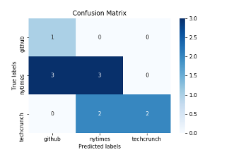
Figure 5-3. A confusion matrix shows all pairs of ground truth labels and predictions so you can explore your model performance within different classes.
Continuous Evaluation
We should make sure the output table also captures the model version and the timestamp of prediction requests so that we can use the same table for continuous evaluation of two different model versions for comparing metrics between the models. For example, if we deploy a newer version of our model, called swivelv2,that is trained on more recent data or has different hyperparameters, we can compare their performance by slicing the evaluation data frame according to the model version:
df_v1 = df_evals[df_evals.version == "swivel"]df_v2 = df_evals[df_evals.version == "swivel_v2"]
Similarly, we can create evaluation slices in time, focusing only on model predictions within the last month or the last week:
today = pd.Timestamp.now(tz='UTC')one_month_ago = today - pd.DateOffset(months=1)one_week_ago = today - pd.DateOffset(weeks=1)df_prev_month = df_evals[df_evals.time >= one_month_ago]df_prev_week = df_evals[df_evals.time >= one_week_ago]
To carry out the above evaluations continuously, the notebook (or containerized form) can be scheduled. We can set it up to trigger a model retraining if the evaluation metric falls below some threshold.
Why It Works
When developing machine learning models there is an implicit assumption that the train, validation and test data come from the same distribution, see Figure 5-4. When we deploy models to production, this assumption implies that future data will be similar to past data. However, once the model is in production “in the wild” this static assumption on the data may no longer be valid. In fact, many production ML systems encounter rapidly changing, non-stationary data, and models become stale over time which negatively impacts the quality of predictions.
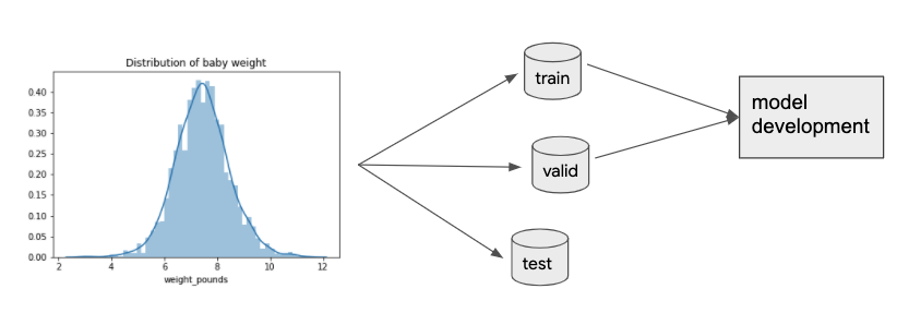
Figure 5-4. When developing a machine learning model the train, validation and test data come from the same data distribution. However, once the model is deployed that distribution can change, severely affecting model performance.
Continuous model evaluation provides a framework to evaluate a deployed model’s performance exclusively on new data. This allows us to detect model staleness as early as possible. This information helps determine how frequently to retrain a model or when to replace it with a new version entirely.
By capturing prediction inputs and outputs and comparing with ground truth, it’s possible to quantifiably track model performance or measure how different model versions perform with A/B testing in the current environment, without regard to how the versions performed in the past.
Tradeoffs and Alternatives
The goal of continuous evaluation is to provide a means to monitor model performance and keep models in production fresh. In this way, continuous evaluation provides a trigger for when to retrain the model. In this case, it is important to consider tolerance thresholds for model performance, the tradeoffs they pose and the role of scheduled retraining. There are also techniques and tools, like TFX, to help detect data and concept drift preemptively by monitoring input data distributions directly.
Triggers for Retraining
Model performance will degrade over time. Continuous evaluation allows you to measure precisely how much in a structured way and provides a trigger to retrain the model. So, does that mean you should retrain your model as soon as performance starts to dip? It depends. The answer to this question is heavily tied to the business use case and should be discussed alongside evaluation metrics and model assessment. Depending on the complexity of the model and ETL pipelines, the cost of retraining could be expensive. The tradeoff to consider is what amount of deterioration of performance is acceptable in relation to this cost.
The threshold itself could be set as an absolute value; for example, model retraining occurs once model accuracy falls below 95%. Or the threshold could be set as a rate of change of performance; for example, once performance begins to experience a downward trajectory. Whichever approach, the philosophy for choosing the threshold is similar to that for checkpointing models during training. With a higher, more sensitive threshold, models in production remain fresh but there is a higher cost for frequent retraining as well as technical overhead of maintaining and switching between different model versions. With a lower threshold, training costs decrease but models in production are more stale. Figure 5-5 shows this tradeoff between the performance threshold and how it affects the number of model retraining jobs.
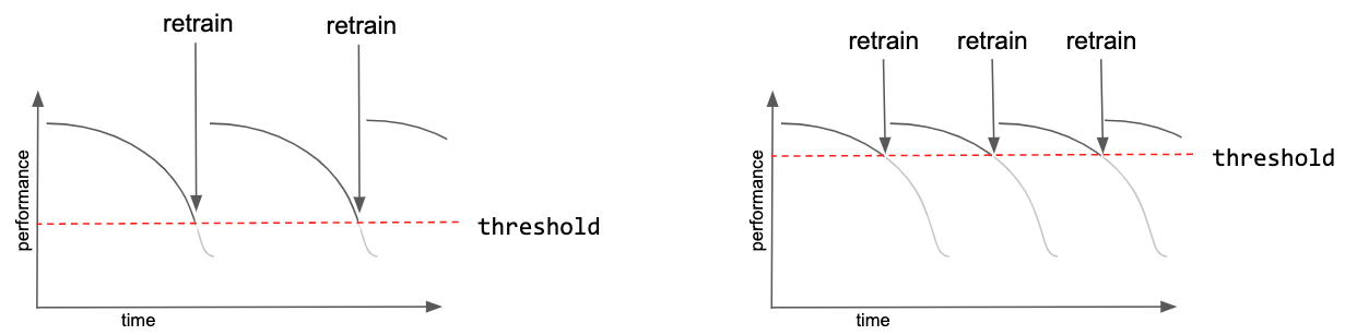
Figure 5-5. Setting a higher threshold for model performance ensures a higher quality model in production, but will require more frequent retraining jobs which can be costly.
If the model retraining pipeline is automatically triggered by such a threshold, it is important to track and validate the triggers as well. Not knowing when your model has been retrained inevitably leads to issues. Even if the process is automated, you should always have control of the retraining of your model to better understand and debug the model in the production.
Scheduled Retraining
Continuous evaluation provides a crucial signal for knowing when it’s necessary to retrain your model. This process of retraining is often carried out by fine tuning the previous model using any newly collected training data. Where continued evaluation may happen every day, scheduled retraining jobs may occur only every week or every month, see Figure 5-6.
Once a new version of the model is trained, its performance is compared against the current model version. The updated model is deployed as a replacement only if it outperforms the previous model with respect to a test set of current data.

Figure 5-6. Continuous evaluation provides model evaluation each day as new data is collected. Periodic retraining and model comparison provides evaluation at discrete time points.
So how often should you schedule retraining? The timeline for retraining will depend on the business use case, prevalence of new data, and the cost (in time and money) of executing the retraining pipeline. Sometimes, the time horizon of the model naturally determines when to schedule retraining jobs. For example, if the goal of the model is to predict next quarter’s earnings, since you will get new ground truth labels only once each quarter, it doesn’t make sense to train more frequently than that. However, if the volume and occurrence of new data is high, then it would be beneficial to retrain more frequently. The most extreme version of this is online machine learning. Some machine learning applications, such as ad placement or newsfeed recommendation, require online, real-time decision and can continuously improve performance by retraining and updating parameter weights with each new training example.
In general, the optimal time frame is something you as a practitioner will determine through experience and experimentation. If you are trying to model a rapidly moving task, such as adversary or competitive behavior, then it makes sense to set a more frequent retraining schedule. If the problem is fairly static, like predicting a baby’s birth weight, then less frequent retrainings should suffice.
In either case, it is helpful to have an automated pipeline set up that can execute the full retraining process with a single API call. Tools like Cloud Composer/Apache Airflow and AI Platform Pipelines are useful to create, schedule and monitor ML workflows from preprocessing raw data and training to hyperparameter tuning and deployment. We discuss this further in the Experiment Pipeline design pattern section in Chapter 6.
Data Validation with TFX
Data distributions can change over time, as in Figure 5-7. For example, consider the natality birthweight dataset. As medicine and societal standards change over time, the relationship between model features, such as the mother’s age or the number of gestation weeks, change with respect to the model label, the weight of the baby. This data drift negatively impacts the model’s ability to generalize to new data. In short, your model has gone stale, and it needs to be retrained on fresh data.
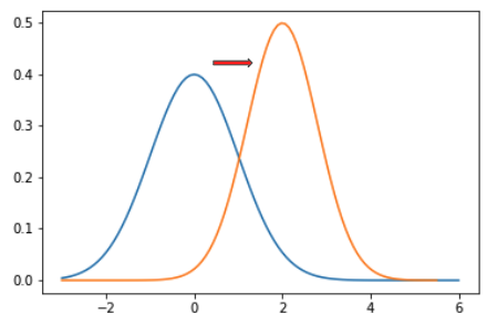
Figure 5-7. Data distributions can change over time. Data drift refers to any change that has occurred to the data being fed to your model for prediction as compared to the data that used for training
While continuous evaluation provides a post-hoc way of monitoring a deployed model, it is also valuable to monitor the new data that is received during serving and preemptively identify changes in data distributions.
TFX’s Data Validation is a useful tool to accomplish this. TFX is an end-to-end platform for deploying machine learning models open sourced by Google. The Data Validation library can be used to compare the data examples used in training with those collected during serving. Validity checks detect anomalies in the data, training-serving skew, or data drift. TensorFlow Data Validation creates data visualizations using Facets, an open source visualization tool for machine learning. The Facets Overview gives a high-level look at the distributions of values across various features and can uncover several common and uncommon issues like unexpected feature values, missing feature values, and training/serving skew.
Estimating Retraining Interval
A useful, and relatively cheap tactic to understand how data and concept drift affect your model is to train a model using only stale data and assess the performance of that model on more current data, see Figure 5-8. This mimics the continued model evaluation process in an offline environment. That is, collect data from 6 months or a year ago and go through the usual model development workflow, generating features, optimizing hyperparameters and capturing relevant evaluation metrics. Then, compare those evaluation metrics against the model predictions for more recent data collected from only a month prior. How much worse does your stale model perform on the current data? This gives a good estimate of the rate at which a model’s performance falls off over time and how often it might be necessary to retrain.
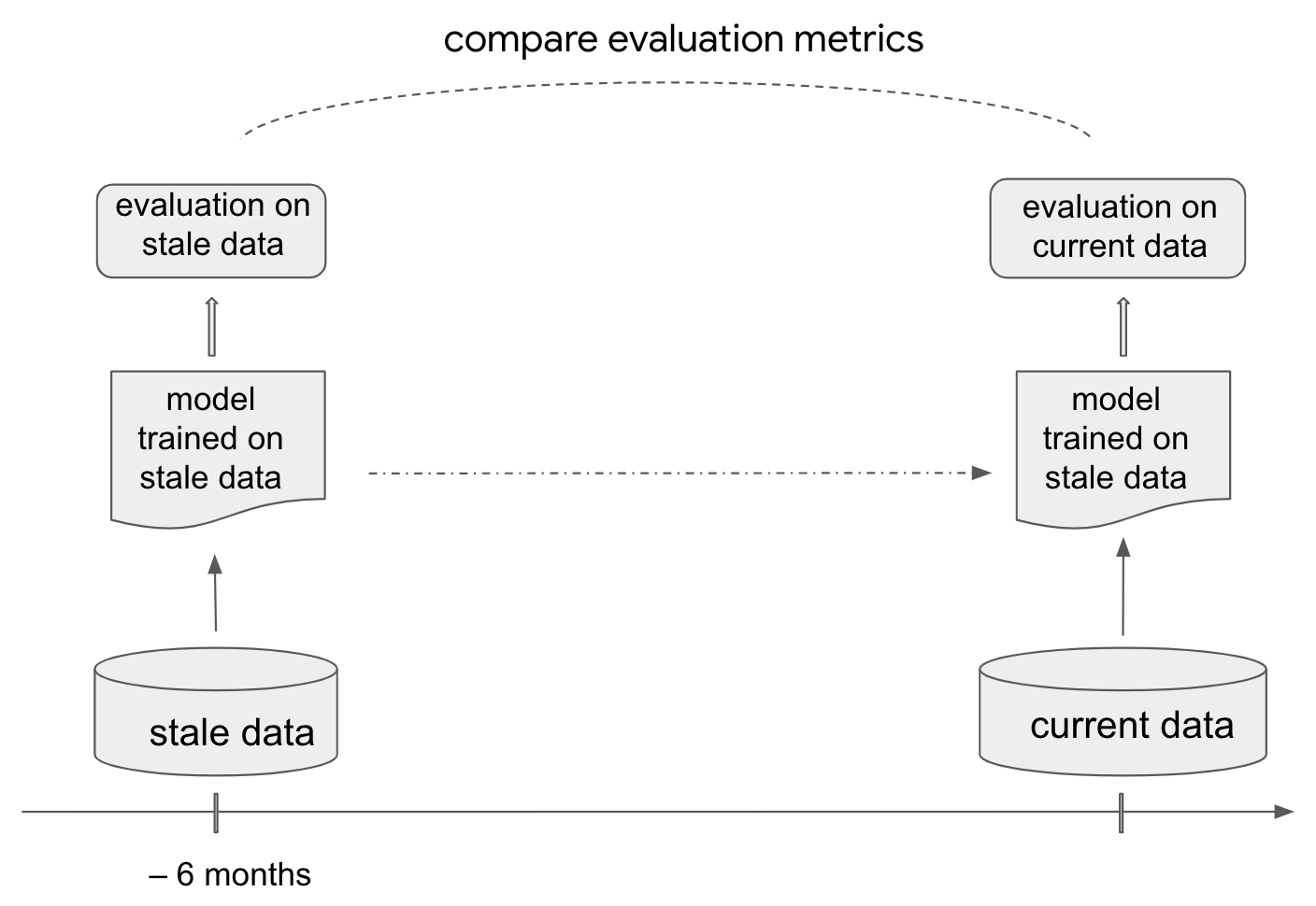
Figure 5-8. Training a model on stale data and evaluating on current data mimics the continued model evaluation process in an offline environment.
Design pattern 19: Two Phase Predictions
The Two Phase Prediction design pattern provides a way to address the problem of keeping large, complex models performant when they have to be deployed on distributed devices by splitting the use cases into two phases, with only the simpler phase being carried out on the edge.
Problem
When deploying machine learning models, we cannot always rely on end users having reliable internet connections. In such situations, models are deployed at the edge – meaning they are loaded on a user’s device and don’t require an internet connection to generate predictions. Given device constraints, models deployed on the edge typically need to be smaller than models deployed in the cloud, and consequently require balancing tradeoffs between model complexity and size, update frequency, accuracy, and low latency.
There are various scenarios where you’d want your model deployed on an edge device. One example is a fitness tracking device, where a model makes recommendations for users based on their activity, tracked through accelerometer and gyroscope movement. It’s likely that a user could be exercising in a remote outdoor area without connectivity. In these cases you’d still want your application to work. Another example is an environmental application that uses temperature and other environmental data to make predictions on future trends. In both of these examples, even if we have internet connectivity, it may be slow and expensive to continuously generate predictions from a model deployed in the cloud.
To convert a trained model into a format that works on edge devices, models often go through a process known as quantization, where learned model weights are represented with fewer bytes. TensorFlow, for example, uses a format called TensorFlow Lite to convert saved models into a smaller format optimized for serving at the edge. In addition to quantization, models intended for edge devices may also start out smaller to fit into stringent memory and processor constraints.
Quantization and other techniques employed by TF Lite significantly reduce the size and prediction latency of resulting ML models, but with that may come reduced model accuracy. Additionally, since we can’t consistently rely on edge devices having connectivity, deploying new model versions to these devices in a timely manner also presents a challenge.
We can see how these tradeoffs play out in practice by looking at the options for training edge models in Cloud AutoML Vision in Figure 5-9.

Figure 5-9. Making tradeoffs between accuracy, model size, and latency for models deployed at the edge in Cloud AutoML Vision.
To account for these tradeoffs, we need a solution that balances the reduced size and latency of edge models against the added sophistication and accuracy of cloud models.
Solution
With the Two Phase Predictions design pattern, we split our problem into two parts. We start with a smaller, cheaper model that can be deployed on-device. Because this model typically has a simpler task, it can accomplish this task on-device with relatively high accuracy. This is followed by a second, more complex model deployed in the cloud and triggered only when needed. Of course, this design pattern requires you to have a problem that can be split into two parts with varying levels of complexity. One example of such a problem is smart devices like Google Home, which are activated by a wake word and can then answer questions and respond to commands related to setting alarms, reading the news, and interacting with integrated devices like lights and thermostats. Google Home, for example, is activated by saying “OK Google” or “Hey Google.” Once the device recognizes a wake word, users can ask more complex questions like “Can you schedule a meeting with Sara at 10am?”.
This problem can be broken into two distinct parts: an initial model that listens for a wake word, and a more complex model that can understand and respond to any other user query. Both models will perform audio recognition. The first model, however, will only need to perform binary classification: does the sound it just heard match the wake word or not? Although this model is simpler in complexity, it needs to be constantly running which will be expensive if it’s deployed to the cloud. The second model will require audio recognition and natural language understanding in order to parse the user’s query. This model only needs to run when a user asks a question, but places more emphasis on high accuracy. Two Phase Predictions can solve this by deploying the wake word model on-device, and the more complex model in the cloud.
In addition to this smart device use case, there are many other situations where Two Phase Predictions can be employed. Let’s say you work on a factory floor where many different machines are running at a given time. When a machine stops working correctly, it typically makes a noise that can be associated with a malfunction. There are different noises corresponding with each distinct machine and the different ways a machine could be broken. Ideally, you can build a model to flag problematic noises and identify what they mean. With Two Phase Predictions, you could build one offline model to detect anomalous sounds. A second cloud model can then be used to identify whether the usual sound is indicative of some malfunctioning condition.
You could also use Two Phase Predictions for an image-based scenario. Let’s say you have cameras deployed in the wild to identify and track endangered species. You can have one model on the device that detects whether the latest image captured contains an endangered animal. If it does, this image can then be sent to a cloud model that determines the specific type of animal in the image.
To illustrate the Two Phase Predictions pattern, let’s employ a general purpose audio recognition dataset from Kaggle. The dataset contains around 9,000 audio samples of familiar sounds with a total of 41 label categories, including “cello,” “knock,” “telephone,” “trumpet,” and more. The first phase of our solution will be a model that predicts whether or not the given sound is a musical instrument. Then, for sounds that the first model predicts are an instrument, we’ll get a prediction from a model deployed in the cloud to predict the specific instrument from a total of 18 possible options. Figure 5-10 shows the two-phased flow for this example:
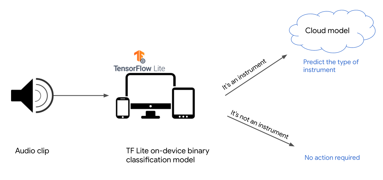
Figure 5-10. Using the Two Phase Predictions pattern to identify instrument sounds.
To build each of these models we’ll convert the audio data to spectrograms, which are visual representations of sound. This will allow us to use common image model architectures along with the Transfer Learning design pattern to solve this problem. See Figure 5-11 for a spectrogram of a saxophone audio clip from our dataset.

Figure 5-11. The image representation (spectrogram) of a saxophone audio clip from our training dataset. Code for converting .wav files to spectrograms can be found in the GitHub repository.
Phase one: Building the offline model
The first model in our Two Phase Prediction solution should be small enough that it can be loaded on a mobile device for quick inference without relying on internet connectivity. Building on the instrument example introduced above, we’ll provide an example of the first prediction phase by building a binary classification model optimized for on-device inference.
The original sound dataset has 41 labels for different types of audio clips. Our first model will only have two labels: “instrument” or “not instrument.” We’ll build our model using the MobileNet V2 model architecture trained on the ImageNet dataset. MobileNet V2 is available directly in Keras, and is an architecture optimized for models that will be served on-device. For our model, we’ll freeze the MobileNet V2 weights and load it without the top so that we can add our own binary classification output layer:
mobilenet = tf.keras.applications.MobileNetV2(input_shape=((128,128,3)),include_top=False,weights='imagenet')mobilenet.trainable = False
If we organize our spectrogram images into directories with the corresponding label name, we can use Keras’s ImageDataGenerator class to create our training and validation datasets:
train_data_gen = image_generator.flow_from_directory(directory=data_dir,batch_size=32,shuffle=True,target_size=(128,128),classes = ['not_instrument','instrument'],class_mode='binary')
With our training and validation datasets ready, we can train the model as we normally would. The typical approach for exporting trained models for serving is to use TensorFlow’s model.save() method. However, remember that this model will be served on-device, and as a result we want to keep it as small as possible. To build a model that fits these requirements, we’ll use TensorFlow Lite, a library optimized for building and serving models directly on mobile and embedded devices that may not have reliable internet connectivity. TF Lite has some built-in utilities for quantizing models both during and after training.
To prepare the trained model for edge serving, we use TF Lite to export it in an optimized format:
converter = tf.lite.TFLiteConverter.from_keras_model(model)converter.optimizations = [tf.lite.Optimize.DEFAULT]tflite_model = converter.convert()open('converted_model.tflite', 'wb').write(tflite_model)
This is the fastest way to quantize a model after training. Using the TF Lite optimization defaults, it will reduce our model’s weights to their 8 bit representation. It will also quantize inputs at inference time when we make predictions on our model. By running the code above, the resulting exported TF Lite model is one-fourth the size it would have been if we had exported it without quantization.
Note
TIP
To further optimize your model for offline inference, you can also quantize your model’s weights during training or quantize all of your model’s math operations in addition to weights. At the time of writing, quantization-optimized training for TensorFlow 2 models is on the roadmap.
To generate a prediction on a TF Lite model, you use the TF Lite interpreter which is optimized for low latency. You’ll likely want to load your model on an Android or iOS device and generate predictions directly from your application code. There are APIs for both platforms, but we’ll show the Python code for generating predictions here so that you can run it from the same notebook where you created your model. First, we create an instance of TF Lite’s interpreter and get details on the input and output format it’s expecting:
interpreter = tf.lite.Interpreter(model_path="converted_model.tflite")interpreter.allocate_tensors()input_details = interpreter.get_input_details()output_details = interpreter.get_output_details()
For the MobileNet V2 binary classification model we trained above, input_details looks like the following:
[{'dtype': numpy.float32,'index': 0,'name': 'mobilenetv2_1.00_128_input','quantization': (0.0, 0),'quantization_parameters': {'quantized_dimension': 0,'scales': array([], dtype=float32),'zero_points': array([], dtype=int32)},'shape': array([ 1, 128, 128, 3], dtype=int32),'shape_signature': array([ 1, 128, 128, 3], dtype=int32),'sparsity_parameters': {}}]
We’ll then pass the first image from our validation batch to the loaded TF Lite model for prediction, invoke the interpreter, and get the output:
input_data = np.array([image_batch[21]], dtype=np.float32)interpreter.set_tensor(input_details[0]['index'], input_data)interpreter.invoke()output_data = interpreter.get_tensor(output_details[0]['index'])print(output_data)
The resulting output is a sigmoid array with a single value in the [0,1] range indicating whether or not the given input sound is an instrument.
Note
TIP
Depending on how costly it is to call your cloud model, you can change what metric you’re optimizing for when you train the on-device model. For example, you might choose to optimize for precision over recall if you care more about avoiding false positives.
With our model now working on-device, we can get fast predictions without having to rely on internet connectivity. If the model is confident that a given sound is not an instrument, we can stop here. If the model predicts “instrument,” it’s time to proceed by sending the audio clip to a more complex cloud-hosted model.
Phase two: Building the cloud model
Since our cloud-hosted model doesn’t need to be optimized for inference without a network connection, we can follow a more traditional approach for training, exporting, and deploying this model. Depending on your Two Phase Prediction use case, this second model could take many different forms. In the Google Home example, phase two might include multiple models: one that converts a speaker’s audio input to text, and a second one that performs NLP to understand the text and route the user’s query. If the user asks for something more complex, there could even be a third model used to provide a recommendation based on user preferences or past activity.
In our instrument example, the second phase of our solution will be a multiclass model that classifies sounds into one of 18 possible instrument categories. Since this model doesn’t need to be deployed on-device, we can use a larger model architecture like VGG as a starting point and then follow the Transfer Learning design pattern outlined in Chapter 4.
We’ll load VGG trained on the ImageNet dataset, specify the size of our spectrogram images in the input_shape parameter, and freeze the model’s weights before adding our own softmax classification output layer:
vgg_model = tf.keras.applications.VGG19(include_top=False,weights='imagenet',input_shape=((128,128,3)))vgg_model.trainable = False
Our output will be an 18-element array of softmax probabilities:
prediction_layer = tf.keras.layers.Dense(18, activation='softmax')
We’ll limit our dataset to only the audio clips of instruments, and then transform the instrument labels to 18-element one-hot vectors. We can use the same image_generator approach above to feed our images to our model for training. Instead of exporting this as a TF Lite model, we can use model.save() to export our model for serving.
To demonstrate deploying the phase two model to the cloud, we’ll use Cloud AI Platform Prediction. We’ll need to upload our saved model assets to a Cloud Storage bucket, and then deploy the model by specifying the framework and pointing AI Platform Prediction to our storage bucket.
Note
TIP
You can use any cloud-based custom model deployment tool for the second phase of the Two Phase Predictions design pattern. In addition to Google Cloud’s AI Platform Prediction, AWS SageMaker and Azure Machine Learning both offer services for deploying custom models.
When we export our model as a TensorFlow SavedModel, we can pass a cloud storage bucket URL directly to the save model method:
model.save('gs://your_storage_bucket/path')
This will export our model in the TF SavedModel format and upload it to our Cloud Storage bucket.
In AI Platform, a model resource contains different versions of your model. Each model can have hundreds of versions. We’ll first create the model resource using gcloud, the Google Cloud CLI:
gcloud ai-platform models create instrument_classification
There are a few ways to deploy your model. We’ll use gcloud and point AI Platform at the storage subdirectory that contains our saved model assets:
gcloud ai-platform versions create v1--model instrument_classification--origin 'gs://your_storage_bucket/path/model_timestamp'--runtime-version=2.1--framework='tensorflow'--python-version=3.7
We can now make prediction requests to our model via the AI Platform Prediction API, which supports online and batch prediction. Online prediction lets us get predictions in near real-time on a few examples at once. If we have hundreds or thousands of examples we want to send for prediction, we can create a batch prediction job that will run asynchronously in the background and output the prediction results to a file when complete.
To handle cases where the device calling our model may not always be connected to the internet, we could store audio clips for instrument prediction on the device while it is offline. When it regains connectivity, we could then send these clips to the cloud-hosted model for prediction.
Tradeoffs and Alternatives
While Two Phase Predictions works for many cases, there are situations where your end users may have very little internet connectivity and you therefore cannot rely on being able to call a cloud-hosted model. In this section we’ll discuss two offline-only alternatives, a scenario where a client needs to make many prediction requests at a time, and suggestions on how to run continuous evaluation for offline models.
Standalone single phase model
Sometimes, the end users of your model may have little to no internet connectivity. Even though these users’ devices won’t be able to reliably access a cloud model, it’s still important to give them a way to access your application. For this case, rather than relying on a two phase prediction flow, you can make your first model robust enough that it can be self-sufficient.
To do this, we can create a smaller version of our complex model, and give users the option to download this simpler, smaller model for use when they are offline. These offline models may not be quite as accurate as their larger online counterparts, but this solution is infinitely better than having no offline support at all. To build more complex models designed for offline inference, it’s best to use a tool that allows you to quantize your model’s weights and other math operations both during and after training. This is known as quantization aware training.
One example of an application that provides a simpler offline model is Google Translate. Google Translate is a robust, online translation service available in hundreds of languages. However, there are many scenarios where you’d need to use a translation service without internet access. To handle this, Google translate lets you download offline translations in over 50 different languages. These offline models are small, around 40 to 50 megabytes, and come close in accuracy to the more complex online versions. Figure 5-12 shows a quality comparison of on-device and online translation models.

Figure 5-12. a comparison of on-device phrase-based and (newer) neural-machine translation models, and online neural machine translation. Source.
Another example of a standalone single phase model is Google Bolo, a speech-based language learning app for children. The app works entirely offline, and was developed with the intention of helping populations where reliable internet access is not always available.
Offline support for specific use cases
Another solution for making your application work for users with minimal internet connectivity is to make only certain parts of your app available offline. This could involve enabling a few common features offline, or caching the results of an ML model’s prediction for later use offline. With this alternative we’re still employing two prediction phases, but we’re limiting the use cases covered by our offline model. In this approach, the app works sufficiently offline, but provides full functionality when it regains connectivity.
Google Maps, for example, lets you download maps and directions in advance. To avoid having directions take up too much space on a mobile device, only driving directions might be made available offline (not walking or biking). Another example could be a fitness application that tracks your steps and makes recommendations for future activity. Let’s say the most common use of this app is checking how many steps you have walked on the current day. To support this use case offline, we could sync the fitness tracker’s data to a user’s device over Bluetooth to enable checking the current day’s fitness status offline. To optimize our app’s performance, we might decide to make fitness history and recommendations only available online.
We could further build upon this by storing the user’s queries while their device is offline, and sending them to a cloud model when they regain connectivity to provide more detailed results. Additionally, we could even provide a basic recommendation model available offline, with the intention of complementing this with improved results when the app is able to send the user’s queries to a cloud-hosted model. With this solution, the user still gets some functionality when they aren’t connected. When they come back online, they can then benefit from a full-featured app and robust ML model.
Handling many predictions in near real-time
In other cases, end users of your ML model may have reliable connectivity but might need to make hundreds or even thousands of predictions to your model at once. If you only have a cloud-hosted model and each prediction requires an API call to a hosted service, getting prediction responses on thousands of examples at once will take too much time.
To understand this, let’s say we have embedded devices deployed in various areas throughout a user’s house. These devices are capturing data on temperature, air pressure, and air quality. We have a model deployed in the cloud for detecting anomalies from this sensor data. Because the sensors are continuously collecting new data, it would be inefficient and expensive to send every incoming data point to our cloud model. Instead, we can have a model deployed directly on the sensors to identify possible anomaly candidates from incoming data. We can then send only the potential anomalies to our cloud model for consolidated verification, taking sensor readings from all the locations into account. This is a variation of the Two Phase Prediction pattern described earlier, the main difference being that both the offline and cloud models perform the same prediction task but with different inputs. In this case, models also end up throttling the number of prediction requests sent to the cloud model at one time.
Continuous evaluation for offline models
How can we ensure our on-device models stay up to date and don’t suffer from data drift? There are a few options for performing continuous evaluation on models that do not have network connectivity. First, we could save a subset of predictions that are received on-device. We could then periodically evaluate our model’s performance on these examples and determine if the model needs retraining. In the case of our two phase model, it’s important we do this evaluation regularly since it’s likely that many calls to our on-device model will not go onto the second phase, cloud model. Another option is to create a replica of our on-device model to run online, only for continuous evaluation purposes. This solution is preferred if our offline and cloud models are running similar prediction tasks, like in the translation case mentioned previously.
Design pattern 20: Keyed Predictions
Normally, you train your model on the same set of input features that the model will be supplied in real-time when it is deployed. In many situations, however, it can be advantageous for your model to also pass through a client-supplied key. This is called the Keyed Predictions design pattern, and it is a necessity to scalably implement several of the design patterns discussed in this chapter.
Problem
If your model is deployed as a web service and accepts a single input, then it is quite clear which output corresponds to which input. But what if your model accepts a file with a million inputs and sends back a file with a million output predictions?
You might think that it should be obvious that the first output instance corresponds to the first input instance, the second output instance to the second input instance, etc. However, with a 1:1 relationship, it is necessary for each server node to process the full set of inputs serially. It would be much more advantageous if you use a distributed data processing system and farm out instances to multiple machines, collect all the resulting outputs, and send them back. The problem with this approach is that the outputs are going to be jumbled. Requiring that the outputs be ordered the same way poses scalability challenges, and providing the outputs in an unordered manner requires the clients to somehow know which output corresponds to which input.
This same problem occurs if your online serving system accepts an array of instances as discussed in the Serving Function pattern. The problem is that processing a large number of instances locally will lead to hot spots. Server nodes that receive only a few requests will be able to keep up, but any server node that receives a particularly large array will start to fall behind. These hot spots will force you to make your server machines more powerful than they need to be. Therefore, many online serving systems will impose a limit on the number of instances that can be sent in one request. If there is no such limit, or if the model is so computationally expensive that requests with fewer instances than this limit can overload the server, you will run into the problem of hot spots. Therefore, any solution to the batch serving problem will also address the problem of hot spots in online serving.
Solution
The solution is to use pass-through keys. Have the client supply a key associated with each input. For example (see Figure 5-13), suppose your model is trained with three inputs (a, b, c), shown on the left, to produce the output d, shown on the right. Make your clients supply (k, a, b, c) to your model where k is a key with a unique identifier. The key could be as simple as numbering the input instances 1, 2, 3, …, etc. Your model will then return (k, d) and so the client will be able to figure out which output instance corresponds to which input instance.
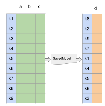
Figure 5-13. The client supplies a unique key with each input instance. The serving system attaches those keys to the corresponding prediction. This allows the client to retrieve the correct prediction for each input even if outputs are out-of-order.
How to pass through keys in Keras
In order to get your Keras model to pass through keys, supply a serving signature when exporting the model.
For example, this is the code to take a model that would otherwise take 4 inputs (is_male, mother_age, plurality, and gestation_weeks) and have it also take a key that it will pass through to the output along with the original output of the model (the babyweight):
# Serving function that passes through keys@tf.function(input_signature=[{'is_male': tf.TensorSpec([None,], dtype=tf.string, name='is_male'),'mother_age': tf.TensorSpec([None,], dtype=tf.float32, name='mother_age'),'plurality': tf.TensorSpec([None,], dtype=tf.string, name='plurality'),'gestation_weeks': tf.TensorSpec([None,], dtype=tf.float32, name='gestation_weeks'),'key': tf.TensorSpec([None,], dtype=tf.string, name='key')}])def keyed_prediction(inputs):feats = inputs.copy()key = feats.pop('key') # get the key from inputoutput =model(feats) # invoke modelreturn{'key': key,'babyweight': output}
This model is then saved as discussed in the Serving Function design pattern:
model.save(EXPORT_PATH,
           signatures={'serving_default': keyed_prediction})
Adding keyed prediction capability to an existing model
Note that the code above works even if the original model was not saved with a serving function. Simply load the model using tf.saved_model.load(), attach a serving function and use the code snippet above, as shown in Figure 5-14.
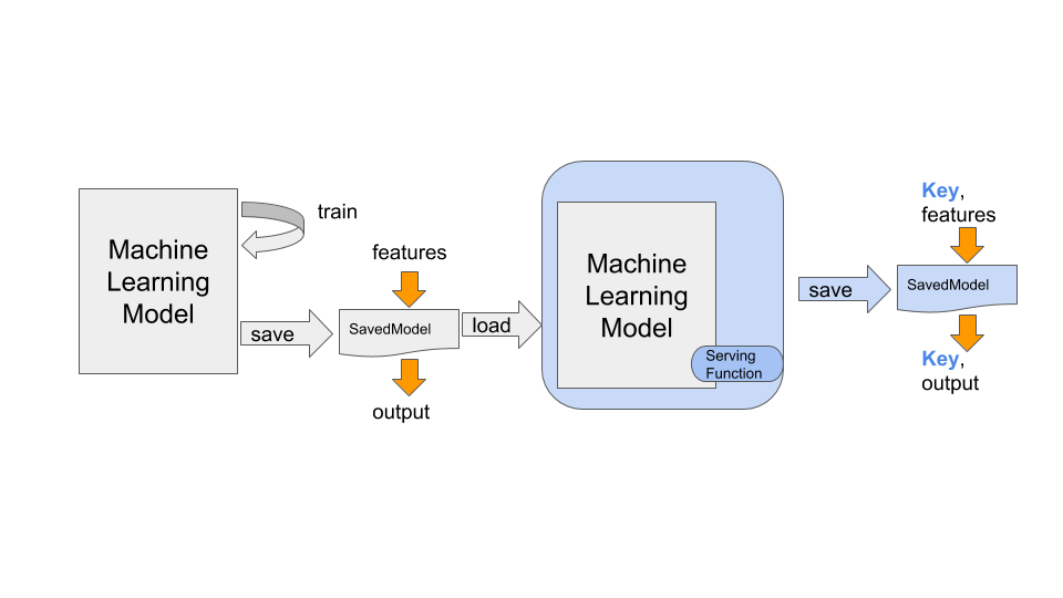
Figure 5-14. Load a SavedModel, attach a non-default serving function and save it.
When doing so, it is preferable to provide a serving function that replicates the older, no-key behavior:
# Serving function that does not require a key@tf.function(input_signature=[{'is_male': tf.TensorSpec([None,], dtype=tf.string, name='is_male'),'mother_age': tf.TensorSpec([None,], dtype=tf.float32, name='mother_age'),'plurality': tf.TensorSpec([None,], dtype=tf.string, name='plurality'),'gestation_weeks': tf.TensorSpec([None,], dtype=tf.float32, name='gestation_weeks')}])defnokey_prediction(inputs):output =model(inputs) # invoke modelreturn{'babyweight': output}
Use the previous behavior as the default and add the keyed_prediction as a new serving function:
model.save(EXPORT_PATH,signatures={'serving_default': nokey_prediction, 'keyed_prediction': keyed_prediction})
Tradeoffs and Alternatives
Why can’t the server just assign keys to the inputs it receives? For online prediction, it is possible for servers to assign unique request ids that lack any semantic information. For batch prediction, the problem is that the inputs need to be associated with the outputs, so the server assigning a unique id is not enough since it can’t be joined back to the inputs. What the server has to do is to assign keys to the inputs it receives before it invokes the model, use the keys to order the outputs, and then remove the keys before sending along the outputs. The problem is that ordering is computationally very expensive in distributed data processing.
In addition, there are a couple of other situations where client-supplied keys are useful — asynchronous serving and evaluation. Given these two situations, it is preferable that what constitutes a key becomes use case specific and needs to be identifiable. Therefore, asking clients to supply a key makes the solution simpler.
Asynchronous serving
Many production machine learning models these days are neural networks, and neural networks involve matrix multiplications. Matrix multiplication on hardware like GPUs and TPUs is more efficient if you can ensure that the matrices are within certain size ranges and/or multiples of a certain number. It can, therefore, be helpful to accumulate requests (up to a maximum latency of course) and handle the incoming requests in chunks. Since the chunks will consist of interleaved requests from multiple clients, the key, in this case, needs to have some sort of client identifier as well.
Continuous evaluation
If you are doing continuous evaluation, it can be helpful to log metadata about the prediction requests, so that you can monitor whether performance drops across the board, or only in specific situations. Such slicing is made much easier if the key identifies the situation in question. For example, suppose that we need to apply a Fairness Lens (see Chapter 7) to ensure that our model’s performance is fair across different customer segments (age of customer and/or race of customer, for example). The model will not use the customer segment as an input, but we need to evaluate the performance of the model sliced by the customer segment. In such cases, having the customer segment(s) be embedded in the key (an example key might be 35-Black-Male-34324323) makes slicing easier.
An alternate solution is to have the model ignore unrecognized inputs and send back, not just the prediction outputs, but also all inputs including the unrecognized ones. This allows the client to match inputs to outputs, but is more expensive in terms of bandwidth and client-side computation.
Because high-performance servers will support multiple clients, be backed by a cluster, and batch up requests to gain performance benefits, it’s better to plan ahead for this — ask that clients supply keys with every prediction and for clients to specify keys that will not cause a collision with other clients.
Summary
In this chapter, we looked at techniques for operationalizing machine learning models to ensure they are resilient and can scale to handle production load. Each resilience pattern we discussed relates to the deployment and serving steps in a typical ML workflow.
We started this chapter by looking at how to encapsulate your trained machine learning model as a stateless function using the Stateless Serving Function design pattern. A serving function decouples your model’s training and deployment environments by defining a function that performs inference on an exported version of your model, and is deployed to a REST endpoint. Not all production models require immediate prediction results, as there are situations where you need to send a large batch of data to your model for prediction but don’t need results right away. We saw how the Batch Serving design pattern solves this by utilizing distributed data processing infrastructure designed to run many model prediction requests asynchronously as a background job, with output written to a specified location.
Next, with the Continued Model Evaluation design pattern, we looked at an approach to verifying that your deployed model is still performing well on new data. This pattern addresses the problems of data and concept drift by regularly evaluating your model, and using these results to determine if retraining is necessary. In the Two Phase Predictions design pattern, we solved for specific use cases where models need to be deployed at the edge. When you can break a problem into two logical parts, this pattern first creates a simpler model that can be deployed on-device. This edge model is connected to a more complex model hosted in the cloud. Finally, in the Keyed Prediction design pattern, we discussed why it can be beneficial to supply a unique key with each example when making prediction requests. This ensures that your client associates each prediction output with the correct input example.
In the next chapter we’ll look at reproducibility patterns. These patterns address challenges associated with the inherent randomness present in many aspects of machine learning, and focus on enabling reliable, consistent results each time a machine learning process runs.
1 Curious what a “positive” complaint looks like? Here you go:
I get phone calls morning XXXX and night. I have told them to stop so many calls but they still call even on Sunday in the morning. I had two calls in a row on a Sunday morning from XXXX XXXX. I received 9 calls on Saturday. I receive about 9 during the week day every day as well.
The only hint that the complainer is unhappy is that they have asked the callers to stop. Otherwise, the rest of the statements might well be about someone bragging about how popular they are!