Let's take a use case and work it out in Python. We are going to use Titanic data from Kaggle.
The data has been split into two groups:

• Training set (train.csv)
• Test set (test.csv)

The data is about the passengers who traveled on the Titanic. It captures their features:

• pclass: Ticket class 1 = 1st, 2 = 2nd, 3 = 3rd
• gender: Gender
• Age: Age in years
• sibsp: Number of siblings/spouses aboard the Titanic
• parch: Number of parents/children aboard the Titanic
• ticket: Ticket number
• fare Passenger: Fare

• cabin: Cabin number
• embarked: Port of embarkation C = Cherbourg, Q = Queenstown, and S = Southampton

We have got to build the model to predict whether or not they survived the sinking of the Titanic. Initially, import the parameters as shown:

import pandas as pd
import numpy as np

We are loading the datasets here:

traindf= pd.read_csv("train.csv")
testdf= pd.read_csv("test.csv")

We have to look for the number of unique values for each variable since BNs are discrete models:

for k in traindf.keys():
 print('{0}: {1}'.format(k, len(traindf[k].unique())))

The output is as follows:

In order to save our system from too much computation and to avoid load on it, we will reduce the number of variables:

for k in traindf.keys():
 if len(traindf[k].unique())<=10:
 print(k)

We get the following  output:

Now, we are left with six variables.

Also, we have to discretize continuous variables in case they needs to be made part of the model:

import math
def forAge(row):
 if row['Age'] < 10:
    return '<10'
 elif math.isnan(row['Age']):
    return "nan"
 else:
    dec = str(int(row['Age']/10))
    return "{0}0's".format(dec)
 decade=traindf.apply(forAge, axis=1)
 print("Decade: {1}".format(k, len(decade.unique())))

The output is as follows:

Let's do the pre-processing now:

def preprocess(df):
 # create a dataframe with discrete variables (len<10)
 filt=[k for k in df.keys() if len(df[k].unique())<=10]
 filtr2=df[filt].copy()
 forAge = lambda row: int(row['Age']/10) if not math.isnan(row['Age']) else np.nan
 filtr2['Decade']=df.apply(forAge, axis=1)
 filtr2=filtr2.dropna()
 filtr2['Decade']=filtr2['Decade'].astype('int32')
 return filtr2

For traindf and testdf, we use the following:

ptraindf= preprocess(traindf)
ptestdf=preprocess(testdf)

ptraindf.to_csv('post_train.csv', index=False)
ptestdf.to_csv( 'post_test.csv', index=False)

df=pd.read_csv('post_train.csv')
for k in df.keys():
  print("{} : {}".format(k, df[k].unique()))

The output can be seen as follows:

import pyAgrum as gum
import pyAgrum.lib.notebook as gnb

Now, it's time to build the model. Here, you need to be watchful while choosing the RangeVariable and LabelizedVariable variables:

template=gum.BayesNet()
template.add(gum.RangeVariable("Survived", "Survived",0,1))
template.add(gum.RangeVariable("Pclass", "Pclass",1,3))
template.add(gum.LabelizedVariable("Gender", "Gender",0).addLabel("female").addLabel("male"))
template.add(gum.RangeVariable("SibSp", "SibSp",0,8))
template.add(gum.RangeVariable("Parch", "Parch",0,9))
template.add(gum.LabelizedVariable("Embarked", "Embarked",0).addLabel('').addLabel('C').addLabel('Q').addLabel('S'))
template.add(gum.RangeVariable("Decade", "Calculated decade", 0,9))
gnb.showBN(template)

The output can be seen as follows:

For learnBN(), we use the following:

learner = gum.BNLearner('post_train.csv', template)
bn = learner.learnBN()
bn

The following is the output:

Now that we have the model, let's try to extract the information from it:

gnb.showInformation(bn,{},size="20")

We get the output as follows:

The entropy of a variable means that the greater the value, the more uncertain the variable's marginal probability distribution is. The lower the value of entropy, the lower the uncertainty. The Decade variable has got the highest entropy, which means that it is evenly distributed. Parch has got low entropy and distribution is non-even.

A consequence of how entropy is calculated is that entropy tends to get bigger if the random variable has many modalities.

Finding the inference gives us a view of the marginal probability distribution here:

gnb.showInference(bn)

The output can be seen as follows:

Now, let's see how classification can be done:

gnb.showPosterior(bn,evs={},target='Survived')

We get the output as follows:

More than 40% of passengers survived here. But, we are not pushing any conditions.

Let's say we want to find out what the chances of a young male surviving are:

gnb.showPosterior(bn,evs={"Gender": "male", "Decade": 3},target='Survived')

The following is the output:

So, the chances are 20.6%.

If we have to find out the chances of an old lady surviving, we go about it as follows:

gnb.showPosterior(bn,evs={"Gender": "female", "Decade": 8},target='Survived')

The output is as follows:

Now, in order to evaluate the model to find out how good it is, we will plot the ROC curve:

from pyAgrum.lib.bn2roc import showROC
 showROC(bn, 'post_train.csv','Survived',"1",True,True)

The following is the output:

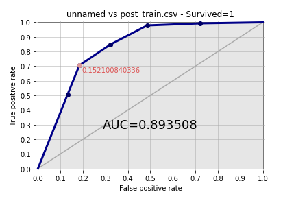
Here, AUC comes out to be 0.893508 and it's quite decent.

We are done with the modeling part here. Also, we have learned about probability theory, Bayesian networks, the calculation of CPT, and how to execute it in Python.