
9
A Threshold-Based Optimization Energy-Efficient Routing Technique in Heterogeneous Wireless Sensor Networks
Samayveer Singh
Department of Computer Science & Engineering, National Institute of Technology Jalandhar, Punjab, India
Abstract
In wireless sensor networks (WSNs), clustering plays the greatest role for persisting the lifespan of the networks and helps in stabilizing the vitality/energy consumption among the existing sensor nodes of the networks. In this paper, a threshold-based optimization energy-efficient direction-finding technique in heterogeneous WSNs is proposed. It considers weighted election probabilities of sensor nodes for electing the master node/cluster heads (CHs). This method also deliberates an approach for transmission of data among the nodes and clusters and data collection in intra- and inter-cluster communication. The performance of the proposed technique is estimated against that of existing protocols using given performance matrices as network lifetime, network stability period, number of CHs, total energy depletion, throughput, etc. The investigational outcomes demonstrate the lifespan of the network, and the throughputs of the suggested method are increased by 25.03%, 31.76%, and 48.91% and 25.38%, 46.02%, and 67.03% in respect of those of hetDEEC-4, EDDEEC-4, and DDEEC-4, respectively, for 100 J network energy in the case of level-4 heterogeneity, correspondingly.
Keywords: Energy efficiency, wireless sensor network, WSNs, clustering, network lifetime, cluster heads
9.1 Introduction
In earlier limited periods, significant development has been done in the arena of wireless sensor networks (WSNs) because of the improvement in the latest technology of sensors. WSNs having or consisting of different abilities link automatic sensing, computing, and communication, and these nodes are easily added into existing networks because of their self-organizing nature [1]. The characteristics of WSNs are self-organizing capability from various failures, constraints of node energies, ease of use, usage of homogeneity and heterogeneity nodes in a defined network, and absorption of various harsh environmental conditions. The sensors are positioned in the observing field for gathering data/information. These sensors collect information from the deployed field and forward the gathered information to other sensor nodes, and then the next node forwards that information to another nearer node. Then, at last, the collected information is communicated to the base station (BS). The BS is unswervingly or indirectly associated with the server with the help of the Internet [2].
Nowadays, WSNs are being deployed in numerous solicitation applications, for example, various fields in health care, water quality monitoring, landslide recognition, industrial and consumer applications, armed reconnaissance, natural disaster deterrence, building/bridge structural health, various types of data centers, forestry fire detection, and data classification. Generally, there are two possible methods to organize/deploy sensors in monitoring fields, namely, deterministic and non-deterministic. The sensors are deployed manually in the case of deterministic deployment, whereas in non-deterministic deployment, sensors are thrown using aircraft or deployed randomly [2].
Sensor networks/systems can be characterized into two comprehensive categories, namely, homogeneous and heterogeneous, depending upon the node’s energy levels and nodes capabilities. Homogeneous networks consist of similar types of sensor nodes, meaning they have the same amount of preliminary vitality/energy, whereas energy is not the same in the situation of heterogeneous networks. The heterogeneous nodes are positioned in all the possible groups in the observing area. These groups are called levels or tiers. The above discussion is founded on the vitality of the sensors; thus, it is called energy heterogeneity. The energy heterogeneity is only possible when the nodes are heterogeneous in the nature. There are two more types of heterogeneity in heterogeneous WSNs, i.e., link and computational heterogeneity [3]. In link heterogeneity, sensors have different-different transmission bandwidth, whereas sensors have different-different computational resources such as the microprocessor in computational heterogeneity as an associate to the normal nodes.
Sensor nodes are restricted due to the limited dimensions, vitality, storing, and cost. Therefore, there is a dire need to design an energy-efficient network to overcome the limitations of sensor networks up to some extent. Clustering shows a vital role for efficient utilization of the limited size, power, storage, and cost of sensor devices. It also helps in efficiently gathering data from the monitoring field using the size of the cluster, the election of CHs, intra and inter-cluster announcement, and data aggregation. Thus, this work is an attempt to determine the problems and provides the solution of energy efficiency by proposing a threshold-based optimization energy-efficient routing technique in heterogeneous WSNs.
The leading influences of the projected work may be itemized as follows: In this work, an innovative methodology for electing the cluster head (CH) by weighted election probabilities of the deployed sensors in heterogeneous WSNs is proposed. This method is capable of selecting the highest energy node with the minimum distance from the base station in the suggested clustering process. It also uses a chain process for gathering information from the nodes inside the clusters and from the cluster heads outside of the cluster and forwards the gathered data to the BS. The proposed heterogeneous model can define four levels of heterogeneity. The various performance matrices are considered for evaluating the performance, which are given as network lifetime and network stability (first node dead), throughput, number of CHs, total energy consumption, etc.
The roadmap of the chapter is given as follows. Section 9.2 discusses the literature review. In Section 9.3, energy and radio models are discussed. In Section 9.4, the proposed model is discussed. Section 9.5 discusses the simulation result and their deliberations. Finally, Section 9.6 concludes the chapter.
9.2 Literature Review
In the last decade and so, there has been a proportion of research on clustering techniques which are established on the load dissemination among nodes to address the energy constraint issue of both homogeneous and heterogeneous networks. The first distributed clustering protocol, which is popularly known as “low-energy adaptive clustering hierarchy” (LEACH), works in two phases, specifically setup and steady-state phases [4]. In the setup phase, the sensor nodes are first grouped into bunches or clusters and then their master node/cluster heads (CHs) are identified. In the steady-state phase, the collected information is conveyed. The LEACH elects CHs arbitrarily using a probability function. To extend the work of LEACH, “power-efficient gathering in sensor information systems” (PEGASIS) forms chains using nodes in WSNs [5]. In the chains, the farthest node gathers data and guides the collected data to its nearer node. The nearer node then forwards the information to a nearer one, and the process continues until the base station receives the information. The PEGASIS protocol is not appropriate for huge-sized systems or networks.
To increase the longevity of the wireless sensor network, a “heterogeneous stable election protocol” (hetSEP) was introduced for 2-level heterogeneity and 3-level heterogeneity [3]. The hetSEP uses functions, namely, weighted election probability and the threshold for CH election and cluster member selection. However, hetSEP may increase overhead in the case of long-distance transmission. For two-level and multilevel energy heterogeneities, the distributed energy-efficient clustering (DEEC) protocol was proposed [6]. The cluster heads are elected using the ratio residual energy of each node and the average energy of the network. Nevertheless, the additional vitality of superior sensor nodes is not professionally consumed, as the vitality is randomly allocated, which leads to infeasibility issues. In [7], the CHs are assigned based on the remaining essentialness of sensors to heightening the lifespan of the WSN if there should be an occurrence of three-level heterogeneity. However, this system requires extra essentialness to remake the groups in each cycle. The convention may endure information misfortune issues in the event of correspondence issues of group heads with one another. To diminish the entomb bunch vitality, Maheswari et al. presented vitality productive two-level grouping convention dependent on the node’s degree [8]. The convention utilizes multi-bounce correspondence, which thusly experiences a surprising burden at the sink. Istwal et al. presented the double group head directing convention for lessening the vitality utilization in WSNs [9]. In any case, convention expends a huge measure of vitality in the inter/bury bunch correspondence. In [10, 11], the energy/vitality, clustering of the sensor nodes is depend on the remaining energy of every sensor node, normal energy, node density, and distance between the sensor nodes and sink. These systems acquire high overhead because of the complex nature of the WSN for bury and intragroup correspondences. Su et al. presented a fluffy-rationale-based vitality effective bunching procedure [12]. The procedure utilizes uneven conveyance of the sensors and the vulnerability of the radio channel utilizing a fluffy rationale for bunch development. The strategy experiences the issue of uneven vitality utilization. Sodairi et al. presented a multi-bounce LEACH for drawing out the vitality lifetime of a WSN [13]. An arbitrary challenge-based vitality compelling group head political decision system was proposed by Narendran et al. which fundamentally uses improved obtrusive weed streamlining (EIWO) metaheuristic for the appointment of bunch heads [14]. Be that as it may, the irregular appointment of CHs builds the correspondence cost. To limit vitality exhaustion between sensors, Ke et al. presented a progressive bunch-based directing convention [15]. The convention utilizes arched capacity with a nonlinear programming issue to locate the ideal arrangement. A circulated vitality productive grouping plan for heterogeneous remote sensor systems is created by Elbhiri et al. [16]. The vitality of this system proficiently chooses CHs utilizing remaining vitality. Javaid et al. examined an improved DEEC conspire for heterogeneous WSNs [17]. This plan proficiently discovers group heads utilizing lingering vitality and political decision likelihood. In the following sections, the heterogeneous energy consumption models will be discussed.
9.3 System Model
In this segment, first deliberate the assumptions made for the projected network and then discuss network and radio energy dissipation models. The basic assumptions are given as follows:
- All the sensors are stationary and have unique ID, and deployed randomly in the monitoring area.
- Nodes can be homogeneous or heterogeneous, and their initial energies rely upon the level of heterogeneity.
- Sensors have symmetric connections, comparative capacities, and constrained computational supremacy, memory, and vitality.
- Base station (BS) is placed in the central of the monitoring filed and sensors and BS distance can be calculated using received signal strength.
- Sensors have self-organising capabilities.
There are three reference models considered in the proposed work, which are as follows: heterogeneous system, radio, and vitality models. The nitty-gritty depiction of the heterogeneous system, radio, and vitality models is given beneath.
9.3.1 Four-Level Heterogeneous Network Model
In this section, a 4-level heterogeneity model that can designate four levels of heterogeneity is discussed. First of all, an N number of sensors are arbitrarily deployed in the characterized observing zone. Fundamentally, sensors are heterogeneous in nature. The heterogeneous sensors have a diverse measure of energy/vitality levels. The heterogeneous nodes might be called level-1, level-2, ..., level-4 nodes. The energies of level-1, level-2, ..., level-4 nodes/hubs are indicated as E0, E1, …, E3, individually, which must fulfill the imbalance E0 < E1 < ⋯ < E3, and their numbers are meant as N1, N2, …, N4, separately, which must fulfill the disparity N1 > N2 > ⋯ > N4. The entire network energy can be calculated as follows:
where ρ is a system constraint.
The nodes’ vitalities are associated as Ei = E0 + θi, i = 1, 2, 3. Where θ1, θ2, θ3 are the parameters.
Putting Ei = E0 + θi in (1), we get
Level-1 Heterogeneity
For θi = 0, i = 1,2,3, the separated framework has just level-1 nodes/hubs; for example, all have similar vitality, and for this situation, the complete system vitality is given by
The number of nodes/hubs in level-1 heterogeneity is given as
The level-1 heterogeneity consists of only single type of nodes means entire nodes consist ofidenticalquantity of energy. So, this network is also called the homogeneous networks.
Level-2 Heterogeneity
For θi = 0, i=2,3, the system has level-1 and level-2 nodes, and for this situation, the complete system vitality is given by
The quantities of level-1 and level-2 nodes, denoted by N1 and N2, correspondingly, are as follows:

with conditions (ρ + ρ2 + ρ3 + ⋯ + ρn) ∗ N = N1, ρ2 ∗ θ1 = N – N1.
Level-3 Heterogeneity
For θi = 0, i=3,4, the system has level-1, level-2, and level-3 nodes, and for this situation, the complete system vitality is given by
The quantities of level-1, level-2, and level-3 nodes, denoted by N1, N2 and N3, correspondingly, are as follows:
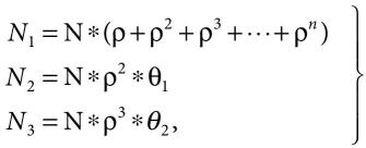
with conditions (ρ + ρ2 + ρ3 +⋯ + ρn) ∗ N = N1, (ρ2 ∗ θ1 + ρ3 ∗ θ2) ∗ N = N – N1.
Level-4 Heterogeneity
For θi = 0, i=4, the system has level-1, level-2, level-3, and level-4 nodes, and for this situation, the complete system vitality is given by
The quantities of level-1, level-2, level-3, and level-4 nodes, denoted by N1, N2, N3 and N4, correspondingly, are as follows:

with conditions (ρ + ρ2 + ρ3 + ⋯ + ρn) ∗ N = N1, (ρ2 ∗ θ1 + ρ3 ∗ θ2 + ρ4 ∗ θ3) ∗ N = N – N1.
9.3.2 Energy Dissipation Radio Model
In this section, a radio dispersal vitality model is talked about. The vitality consumption for communicating L-bit data over the short (ETXS) and long (ETXL) separation d is assumed as follows [4]:
where ∈elec, ∈fs, and ∈mp are the vitality scattered and d0 is the separation limit between a sensor and the BS as given below:

The absolute vitality devoured by the transmitter in advanced coding and adjustment is characterized in the principal term of (7) and (8). The energies spent in getting (ERx) and in detecting (ESx) are yielded (10) and (11) as follows:
9.4 Proposed Work
In this section, a description of optimum cluster head election, chain-based information congregation and communication procedure for intra and inter-cluster announcement, and employed procedure of the proposed method is discussed.
9.4.1 Optimum Cluster Head Election of the Proposed Protocol
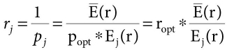
In this section, the selection of the cluster heads for the proposed method is discussed as follows. The heterogeneous distributed energy-efficient clustering (hetDEEC) protocol is considered for evaluating the performance of the suggested four-level network model, which is one of the important protocols [7]. Let us consider that the average number of CHs is N ∗ popt and a node becomes a CH after rj = 1/popt rounds, where popt and rj are the optimal probability to become a CH of a node and the number of rounds, respectively. The network average vitality E r( ) for round r is as follows:

The average probability of a node to be CH is given as follows:

where Ei(r) is residual energy and the total CHs are given as follows:

In this scenario, a sensor node has more chance to become a CH if it has the highest residual energy among the sensors. Equation 2 defines the total vitality of the heterogeneous system as N ∗ ((ρ + ρ2 +ρ3 + ⋯ + ρn) + ρ2 ∗ θ1 + ρ3 ∗ θ2 + ρ4 ∗ θ3). It chooses N ∗ popt nodes as the average number of CHs which help in minimizing the energy dissipation among the nodes. In this networks, every sensor becomes a cluster head after 1/popt ∗ ((ρ + ρ2 + ρ3 + ⋯ + ρn) + ρ2 ∗ θ1 + ρ3 ∗ θ2 + ρ4 ∗ θ3) rounds. It is also equal to ((ρ + ρ2 + ρ3 + ⋯ + ρn) + ρ2 ∗ θ1 + ρ3 ∗ θ2 + ρ4 ∗ θ3) ∗ N ∗ plevel−1, where plevel−1 is the probability of the level-1 sensor nodes. For differentiating the threshold value, incorporate the level of heterogeneity (as level-1, -2, -3, -4) in the threshold formula to become a CH after N ∗ popt rounds. In the case of level-1 heterogeneity, every sensor node becomes a CH once in every ((ρ + ρ2 + ρ3 + ⋯ + ρn) + ρ2 ∗ θ1 + ρ3 ∗ θ2 + ρ4 ∗ θ3)/popt rounds. Similarly, each level-2 node becomes a CH (1 + α) times more than the level-1 node in every ((ρ + ρ2 + ρ3 + ⋯ + ρn) + ρ2 ∗ θ1 + ρ3 ∗ θ2 + ρ4 ∗ θ3)/popt round, and each level-3 and level-4 node becomes a CH (1 + β) and (1 + γ) times more than the level-1 nodes in every ((ρ + ρ2 + ρ3 + ⋯ + ρn) + ρ2 ∗ θ1 + ρ3 ∗ θ2 + ρ4 ∗ θ3)/popt and ((ρ + ρ2 + ρ3 + ⋯ + ρn) + ρ2 ∗ θ1 + ρ3 ∗ θ2 + ρ4 ∗ θ3)/popt round, respectively.
The proposed approach gives weights for each type of heterogeneity to obtain optimal probability. By using (15), weighted probabilities are calculated. The weighted probabilities of the level-1, -2, -3, and -4 nodes for the proposed method, denoted by plevel−1, plevel−2, plevel−3, and plevel−3, respectively, are given by
The choice of CH is based on the likelihood formula, which is specified as follows:

Where popt and G are the predetermined % of CHs and set of nodes that have not been CHs in the last 1/popt rounds.
Election of CH in each round can be calculated by putting the value of the plevel−1, plevel−2, plevel−3, and plevel−4 in (19). Thus, the thresholds T(sj) for level-1, level-2, level-3, and level-4 are given by

where G′, G″, G‴, and G″″ are conventional of level-1, -2, -3, and -4 nodes that have not become CHs within the last 1/pnrm, 1/padv, 1/psup and 1/pusup rounds, respectively.
9.4.2 Information Congregation and Communication Process Based on Chaining System for Intra and Inter-Cluster Communication
Stage 1. Compute the distance of each sensor from the CHs and distance among the other sensors in the cluster or distance amongst each CHs and the BS in the specified network.
Stage 2. Select the furthest sensor node from the cluster head (CH)/BS which will be the first sensor/ cluster head node of the intra/inter communication chaining process in the clusters/networks.
Stage 3. The farthest sensor/CH begins to pick the following sensor/ CH to develop the chain by considering the eager approach. This methodology considers the base far-off sensor/group head node as the following node from the farthest node. Correspondingly, the subsequent least far-off sensor/group head node is picked. This procedure proceeds until the following least far-off node/bunch head is the group head/systems.
Stage 4. After forming the first chain in the cluster/networks, if any sensor/ CH node is not connected with the respective cluster head/base station then construction of a new chain will start by consider the same process as defined in Step 3 in the cluster/networks distinctly.
Stage 5. When the energy of a sensor/cluster head become zero means the sensor/cluster headexpires in the chain and the chain is again reassembled to avoid the dead node/cluster head.
Stage 6. Repeat Step 1 to Step 5 for all the possible clusters.
9.4.3 The Complete Working Process of the Proposed Method
In this section, the total portrayal working procedure of an upgrade vitality effective steering method in heterogeneous WSNs is talked about, which aids in prolonging the network/system lifespan. The proposed method is worked into two stages: setup/arrangement and steady/unfaltering state stages.
Setup Phase
In the arrangement stage, at first, a remote system is framed, and afterward, the method for appointment of CH node is prepared. The bit-by-bit arrangement is examined as follows.
Stage 1. First of all, an N number of sensors are arbitrarily deployed in the characterized observing zone. Fundamentally, sensors are heterogeneous in nature. The heterogeneous nodes have the diverse measure of energy/vitality levels. The heterogeneous nodes might be called as level-1, level-2, ..., level-4 nodes. The energies of level-1, level-2, ..., level-4 nodes/hubs are indicated as E0, E1,…, E3 individually, which must fulfill the imbalance E0 < E1 < ⋯ < E3, and their numbers are meant as N1, N2,…, N4 separately, which must fulfill the disparity N1 > N2 > ⋯ > N4. A solitary BS is conveyed in the observing zone which gathers the information from each group head.
Stage 2. After network formation, procedure for election of CHs discussed in section 9.4.1
Steady-State Phase
After CH determination, the genuine information accumulation and communications to the CHs and the BS happen in the steady/consistent state stage. This procedure is talked about in the accompanying advances.
Stage 1. Subsequently in the CHs election, each CH starts the process of chain construction in the respective cluster for intra-cluster communications. The chain construction is constructed on the distance among the nodes and the CH which is calculated by the RSSI.
Stage 2. After forming the chain within the cluster intra-cluster communication starts. In the intra cluster announcement farthest node join itself as the first node in the chain and starts to collect the information and forwards it to the nearest node.
Stage 3. The selection of the nearest node from the farthest sensor node is grounded on the minimum distant node in the chain and once a node is already in the chain will not be consider again. The CHsreceived the data from the respective sensors in each cluster after chain construction process.
Stage 4. After intra cluster communication data gathering process from each cluster, the inter-cluster communication takes place. In this process, all cluster heads adopted both single hop and multi-hop communication and direct their information to the BS using the same chaining approach similar as intracommunication by considering the sink as cluster head.
Stage 5. In this proposed method, each sensor and cluster node perform the data aggregation in both inter- and intra-cluster communication in order to removal of the duplicate data.
Stage 6. Moreover, on the off chance that the leftover vitality of any node has become zero, at that point the node/hub is said to be a dead hub and it is erased from the networks/systems. Notwithstanding, when every sensor is dead, the system stops working.
9.5 Simulation Results and Discussions
In this section, the re-enactment consequences of the proposed methods and the current DEEC convention variations are contrasted. The deterministic energy-efficient clustering (DEEC) chooses CHs by utilizing the proportion of lingering energy/vitality of every sensor and normal vitality of the network. It does not utilize the additional vitality of more elevated level nodes effectively, as the vitality of the nodes is haphazardly assigned from a given vitality interim. In this manner, it cannot be achievable to structure such a network. The proposed convention is the changed execution of DEEC using limit remaining vitality for cluster head determination. It chooses higher remaining vitality sensors for cluster/bunch head in an effective way. The projected strategy is executed utilizing transmission and accumulation of information, and a chain-based information social occasion and communication procedure for intra- and between-cluster/bunch correspondence. All the planned executions are functional on four-level heterogeneous systems for assessing the exhibition. The trial arrangement for all the projected and existing conventions is given beneath.
The networks are reproduced in MATLAB adaptation R2014. The proposed network system comprises 100 heterogeneous nodes which are in an irregular arrangement in a square field of measurement 100 m × 100 m in every one of the reproductions. The BS is situated in the checking region at measurement 50 m × 50 m, and the underlying energy/vitality of the typical or level-1 nodes is 0.50 J. The outcomes introduced are the found middle value of the 20-recreation run by thinking about similar parameters. We deliberate distinctive execution grids for assessing the exhibition of the proposed technique against the other existing conventions given as follows: network lifetime, network sustainability, complete energy/vitality utilization, throughput, and the number of bunch heads.
For a similar investigation of the reproduction results, a heterogeneous system is considered. The proposed heterogeneous system comprises four types of nodes, in particular level-1, -2, -3, and -4 networks. This network contains level-4 heterogeneity where the quantity of level-1 (N1) nodes, level-2 (N2) nodes, level-3 (N3) nodes, and level-4 (N4) nodes are 46, 27, 16, and 11, with their energies as 0.50 J (E0), 1.25 J (E1), 1.75 J (E2), and 2 J (E3), correspondingly. Consider energy disbursed by amplifier to transmit data at shorter (∈fs) and longer distance (∈mp) and the energy consumption to transmit or receive signal (∈elec) are 10nJ/bit/m2, 0.0013pJ/bit/m4, and 50nJ/bit, respectively. Additionally, think that the vitality for information conglomeration (∈DA), threshold separation (d0), message size (L), and vitality steady (δ) are 5nJ/bit/ signal, 70 m, 4000 bits, and 1.5, separately.
In this section, the exhibition assessment of the DDEEC [16], EDDEEC [17], hetDEEC-4 [7], and proposed strategy conventions are talked about for heterogeneous networks. We have considered four degrees of heterogeneity for breaking down the presentation of the networks. The outcomes for various frameworks such as network lifespan, vitality utilization, throughput, and the quantity of group heads are assumed as follows.
9.5.1 Network Lifetime and Stability Period
Figure 9.1 shows the number of alive nodes in regard to the number of rounds for DDEEC-4 [16], EDDEEC-4 [17], hetDEEC-4 [7], and proposed strategy in level-4 networks. It is seen that the proposed technique covers 7002 rounds though hetDEEC-4, EDDEEC-4, and DDEEC-4, spread 5600, 5314, and 4702 rounds, individually, before exhausting the total energy/ vitality of the considerable number of nodes. In this way, the proposed technique increments 25.03%, 31.76%, and 48.91% in the lifespan of the network in regard to hetDEEC-4, EDDEEC-4, and DDEEC-4, separately. The proposed limit leftover energy/vitality helps to increase the lifespan of the network since the node distance decreases the correspondence cost between the sensors and BS. Moreover, the nodes in the proposed method die leisurelier than the hetDEEC-4, EDDEEC-4, and DDEEC-4 because it chooses the head nodes proficiently which helps in extending the network lifespan. It is also evident from the Figure 9.1; any increases in tire of heterogeneity show a significant increment in the network lifespan. Figure 9.2 demonstrates the number of dead nodes in regard of the number of rounds for DDEEC-4 [16], EDDEEC-4 [17], hetDEEC-4 [7], and proposed strategy in level-4 networks. It is showing similar behaviour as presented in Figure 9.2.

Figure 9.1 Alive nodes vs number of rounds.
The economical time of the proposed technique is 2831, 3208, and 7002, individually, for first node dead as demonstrated in Figure 9.3 in level-4 systems. It is evident from the Figure 9.3 the sustainable period of the proposed method for first node dead significantly exceeds by 19.04%, 41.26%, and 59.85% as comparison with the hetDDEEC-4, EDDEEC-4, and DDEEC-4, respectively because the proposed methods considered the threshold residual energy. The weighted election decision probabilities guarantee the base vitality consumption in the intra- and inter/bury cluster/bunch transmission among the sensors and the base station. It is manifest the sustainable period of the proposed significantly exceeds by 18.37%, 36.56%, & 59.92% and 25.03%, 31.76%, &48.91%as comparison with the hetDDEEC-4, EDDEEC-4,& DDEEC-4, respectively, for half and last node dead, separately. Along these lines, this vitality protection helps in the supportability of the systems. Figure 9.3 shows as the tire of heterogeneity increase the network lifespan of the increases.

Figure 9.2 Dead nodes vs number of rounds.

Figure 9.3 First node dead (FND), half node dead (HND), and last node dead (LND) vs number of rounds.
9.5.2 Network Outstanding Energy
The normal energy/vitality dissemination of the DDEEC-4, EDDEEC-4, hetDDEEC-4, and proposed strategies in regard of the quantity of rounds is demonstrated in Figure 9.4 in the level-4 systems. The beginning vitality of the system is considered as 107 J. The proposed method outperforms as compare to the DDEEC-4, EDDEEC-4, and hetDDEEC-4 because it covers more number of rounds. The results show the higher energy consumption in DDEEC-4, EDDEEC-4,and hetDDEEC-4 because they do not consider any chaining approach for data transmission among the nearby nodes and BS. Moreover, the proposed method considers both intra and inter cluster communication by chaining approach which preserves energy of the sensors in the effective manner. Along these lines, it decreases the computational vitality cost of the CHs in the systems. It is likewise clear that as the tier of heterogeneity expands, the vitality consumption diminishes as demonstrated in Figure 9.4.
9.5.3 Throughput
The quantity of packets acknowledged by the BS in respect of the quantity of rounds till the networks alive using the DDEEC-4, EDDEEC-4, hetDDEEC-4, and proposed strategies is indicated in Figure 9.5. The proposed strategy sent 25.38%, 46.02 %, and 67.03% progressively the number of packets to the BS regarding hetDEEC-4, EDDEEC-4, and DDEEC, separately. It is likewise seen that the proposed technique sent information packets at a higher rate to the BS as related to DDEEC-4, EDDEEC-4, and hetDDEEC-4. The proposed technique produces the most elevated number of packets because the nodes in the proposed strategy stay alive more as far as the number of rounds.

Figure 9.4 Energy consumption vs number of rounds.

Figure 9.5 Packets sent to BS vs number of rounds.
Table 9.1 Illustrations of the total energy of the network, FND, HND, LND, throughput, increment % in lifetime, and throughput for the proposed method, hetDEEC-4, EDDEEC-4, and DDEEC-4 for four levels of heterogeneity.
| Results for tier-4 network protocols | |||||||
| Approaches | Total energy | FND | HND | LND | Throughput | % increment in lifetime | % increment in throughput |
| Proposed method | 107 | 2831 | 3208 | 7002 | 62185 | – | – |
| hetDEEC-4 | 107 | 2378 | 2710 | 5600 | 49597 | 25.03 | 25.38 |
| EDDEEC-4 | 107 | 2004 | 2349 | 5314 | 42584 | 31.76 | 46.02 |
| DDEEC-4 | 107 | 1771 | 2006 | 4702 | 37228 | 48.91 | 67.03 |
9.5.4 Comparative Analysis of the Level-4 Network Protocols
Table 9.1 demonstrates the relative examination of the absolute network power, first node dead (FND), half node dead (HND), last node dead (LND), throughput, rate increase in lifetime, and throughput for the proposed strategy and the current strategies, for example, hetDEEC-4 [7], EDDEEC-4 [17], and DDEEC-4 [16], separately by considering level-4 heterogeneity. If there should arise an occurrence of level-4 heterogeneity, the network lifetime and throughput of proposed strategy are expanded by 25.03%, 31.76%, and 48.91% and 25.38%, 46.02 %, and 67.03 % in regard of hetDEEC-4, EDDEEC-4, and DDEEC-4, separately, using network energy of 107 J, individually. It is shown from Table 9.1 that the supportable time of the proposed technique fundamentally increases by 19.04%, 41.26%, and 59.85%; 18.37%, 36.56%, and 59.92%; and 25.03%, 31.76%, and 48.91% as examination with hetDEEC-4, EDDEEC-4, and DDEEC-4, separately, for first, half, and last node dead, individually, for level-4 heterogeneity. The proposed strategy performs best among hetDEEC-4, EDDEEC-4, and DDEEC-4, separately, on the grounds that it accomplishes burden adjusting by considering weighted political election probabilities-based grouping and fastening approach. Thus, it is evident from the results weighted election probabilities based clustering and chaining approach enhance the reliability and also improve the sustainable period of the networks in the cases of four level of heterogeneity.
9.6 Conclusion
In this paper, a threshold-based optimization energy-efficient directing method for prolonging the lifespan of the network in a heterogeneous environment is proposed. The proposed protocol used weighted election probabilities for CH election and a chaining approach for proficient information/data gathering. The proposed method delivers a sustainable region for heterogeneous networks since it elects the highest energy nodes for CH efficiently. The network lifetime and throughput of the proposed method are presented as increased by 25.03%, 31.76%, and 48.91% and 25.38%, 46.02%, and 67.03% in respect of hetDEEC-4, EDDEEC-4, a DDEEC-4, using 107 J network energy in the case of level-4 heterogeneity, respectively. The proposed method performs best among hetDEEC-4, EDDEEC-4, and DDEEC-4. The simulation results of the proposed method also show that as the level of heterogeneity increased, the lifespan of the networks increased, accordingly. This work can be extended using multiple sinks instead of single and mobile sinks, and sensors can be added for monitoring the different applications.
References
- 1. Chand, S., Singh, S., Kumar, B., Heterogeneous HEED Protocol for Wireless Sensor Networks. Wireless Pers. Commun., 77, 3, 2117–2139, 2014.
- 2. Singh, S., Chand, S., Kumar, R., Malik, A., Kumar, B., NEECP: Novel energy-efficient clustering protocol for prolonging lifetime of WSNs. IET Wireless Sens. Syst., 6, 5, 151–157, 2016.
- 3. Singh, S. and Malik, A., hetSEP: Heterogeneous SEP protocol for increasing lifetime in WSNs. J. Inf. Optim. Sci., 38, 5, 721–743, 2017.
- 4. Heinzelman, W.R., Chandrakasan, A.P., Balakrishnan, H., An application-specific protocol architecture for wireless microsensor networks. IEEE Trans. Wireless Commun., 1, 4, 660–670, 2002.
- 5. Lindsey, S., Raghavendra, C.S., Sivalingam, K.M., Data gathering algorithms in sensor networks using energy metrics. IEEE Trans. Parallel Distrib. Syst., 13, 9, 924–935, 2002.
- 6. Qing, L., Zhu, Q., Wang, M., Design of a distributed energy-efficient clustering algorithm for heterogeneous wireless sensor networks. Comput. Commun., 29, 12, 2230– 2237, 2006.
- 7. Singh, S., Malik, A., Kumar, R., Energy efficient heterogeneous DEEC protocol for enhancing lifetime in WSNs. Eng. Sci. Technol., an International Journal, 20, 1, 345–353, 2017.
- 8. Maheswari, D.U. and Sudha, S., Node Degree Based Energy Efficient Two-Level Clustering for Wireless Sensor Networks. Wireless Pers. Commun., 104, 3, 1209–1225, 2018.
- 9. Istwal, Y. and Verma, S.K., Dual Cluster Head Routing Protocol with Super Node in WSN. Wireless Pers. Commun., 104, 2, 561–575, 2019.
- 10. Singh, S., Chand, S., Kumar, B., Multilevel heterogeneous network model for wireless sensor networks. Telecommun. Syst., 64, 2, 259–277, 2017.
- 11. Singh, S., Chand, S., Kumar, B., Energy-efficient protocols using fuzzy logic for heterogeneous WSNs. Wireless Pers. Commun., 86, 2, 451–475, 2017.
- 12. Su, S. and Zhao, S., An optimal clustering mechanism based on Fuzzy-C means for wireless sensor networks. Sustain. Comput.: Informat. Syst., 18, 127–134, 2018.
- 13. Sodairi, S.A. and Ouni, R., Reliable and energy-efficient multi-hop LEACH-based clustering protocol for wireless sensor networks. Sustain. Comput.: Informat. Syst., 20, 1–13, 2018.
- 14. Narendran, M. and Prakasam, P., An energy aware competition based clustering for cluster head selection in wireless sensor network with mobility. Cluster Comput., 22, 11019–11028, 2019.
- 15. Ke, W., Yangrui, O., Hong, J., Heli, Z., Xi, L., Energy aware hierarchical cluster-based routing protocol for WSNs. J. China Univ. Posts Telecommun., 23, 4, 46–52, 2016.
- 16. Elbhiri, B., Saadane, R., El Fkihi, S., Aboutajdine, D., Developed Distributed Energy-Efficient Clustering (DDEEC) for heterogeneous wireless sensor networks. 5th International Symposium on I/V Communications and Mobile Network (ISVC), 2010.
- 17. Javaid, N., Qureshi, T.N., Khan, A.H., Iqbal, A., Akhtar, E., Ishfaq, M., EDDEEC: Enhanced Developed Distributed Energy-Efficient Clustering for Heterogeneous Wireless Sensor Networks. International Workshop on Body Area Sensor Networks (BASNet-2013).
Note
- Email: [email protected]