
12. Dimensional Reduction and Latent Variable Models
12.1 Introduction
Now that you have the tools for exploring graphical models, we’ll cover a few useful ones. We’ll start with factor analysis, which finds application in the social science and in recommender systems. We’ll move on to a related model, principal components analysis, and explain how it’s useful for solving the collinearity problem in multiple regression. We’ll end with ICA, which is good for separating signals that have blended together. We’ll explain its application on some psychometric data.
One thing all of these models have in common is that they’re latent variable models. That means in addition to the measured variables, there are some unobserved variables that underlie the data. You’ll understand what this means more deeply in the context of these models.
We’ll only really scratch the surface of these models. You can find a lot more detail in Murphy’s Machine Learning: A Probabilistic Perspective [24]. Before we go into a few models, let’s explore an important concept: a “prior” for a variable.
12.2 Priors
Let’s talk about making a measurement of a click-through rate on a website. When you show a link to another section of the website, it’s called an impression of that link. When a user receives an impression, they can either click the link or not click it. A click will be considered a “success” and a noisy indication that the user likes the content of the page. A nonclick will be considered a “failure” and a noisy indication that the user doesn’t like the content. The click-through rate is the probability that a person will click the link when they receive an impression, p = P(C = 1|I = 1). You can estimate it by looking at .
If you serve one impression of a link and the user doesn’t click it, your estimate for will be 0/1 = 0. You’d guess that every following user will definitely not click the link! Clearly, that is a pathological result and can cause problems. What if your recommendation system was designed to remove links that performed below a certain level? You’d have some real trouble keeping content on the site.
Fortunately, there’s a less pathological way to learn the click-through rate. You can take a prior on the click rate. To do this, you look at the distribution of all of the past values of the click rates (even better, fit a distribution to it with MCMC!). Then, having no data on a click rate, you at least know that it’s drawn from that past distribution, as shown in Figure 12.1.
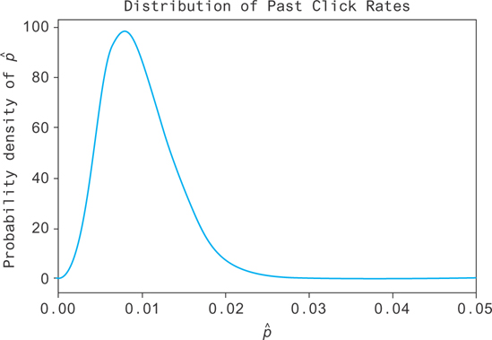
Figure 12.1 The distribution of click-through rates for past hyperlinks
This distribution represents your prior knowledge of the click-through rate, in the sense that it’s what you know before you collect any data. You know here, for example, that you’ve never seen a link with a click rate as high as p = 0.5. It’s extremely unlikely that the current link performs that well.
Now, as you collect data, you want to update your prior with new information. The resulting distribution will be called a posterior density for p. Suppose the true value is p = 0.2. After 20 impressions you get a posterior that looks like Figure 12.2. You can see the distribution is narrow, so you’re slightly more sure that the true value lies in a smaller range. The distribution has also shifted more to the right, closer to the true value of p = 0.2. This represents the state of our knowledge after incorporating what you’ve learned from the new data with what you knew from the past data!
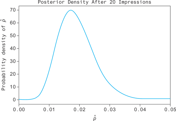
Figure 12.2 Your confidence in the click rate of the current item, given your knowledge of past click rates as well as your new data
Mathematically, the way this works is that you say the prior, P(p), takes on some distribution that you’ve fit using past data. In this case, it’s a beta distribution with parameters to give an average value of around 0.1, with a little variance around it. You can denote this by p Beta (α, β), which you can read as “p is drawn from a beta distribution with parameters α and β.”
Next, you need a model for the data. You can say that an impression is an opportunity for a click, and the click is a “success.” That makes the clicks a binomial random variable, with success probability p and I trials: one for each impression. You can say that it takes the distribution P(C|p, I) and that C|p, I Bin(I, p). Knowing p and I, C is drawn from a binomial distribution with parameters I and p.
Let’s assume impressions are a fixed parameter, I. You can say the distribution for p given I and C (our data) is (by Bayes’ theorem and the chain rule for conditional probability). You can see that the data, C and I, is used to update the prior, P(p) by multiplication to get P(p|I,C).
It’s a fun exercise to derive this posterior and see what distribution it simplifies to!
12.3 Factor Analysis
Factor analysis tries to model N observed k-dimensional vectors, xi, by describing each data point with a smaller set of f < k unmeasured (latent) variables. You write the data points as being drawn from a distribution, as follows:
where θ represents all of the parameters θ = (W, z, μ). W is a k by f matrix, where there are f latent variables. μ is a global mean for the xi, and ψ is the k by k covariance matrix.
The matrix W describes how each factor in z contributes to the values of the components of xi. It’s said to describe how much the factors load on to the components of xi and so is called the factor loading matrix. Given a vector of the values of the latent variables that correspond to a data point x, W transforms z to the (mean-centered) expected value of x.
The point of this is to use a model that is simpler than the data, so the major simplifying assumption that you’ll make is that the matrix ψ is diagonal. Note that this doesn’t mean that the covariance matrix for xi is diagonal! It’s the conditional covariance matrix, when you know zi, which is diagonal. This is going to mean that zi is going to account for the covariance structure in xi.
Importantly, the latent factors z characterize each data point. It’s a condensed representation of the information in the data. This is where factor analysis is useful. You can map from high-dimensional data down to much lower dimensional data and explain most of the variance using much less information.
You use a normal prior for the z variables in factor analysis, zi∽ (μ0, Σ0). This makes it so it’s easy to calculate the posterior for xi. You’ll denote the PDF of the normal distribution with mean μ and covariance matrix Σ as a function of x as (x; μ, Σ). Then, you can find the posterior for xi as follows:
You can actually get rid of the Wμ0 term by absorbing it into the fitted parameter μ. You can also turn the Σ0 term into I, since you’re free to absorb the Σ0 into W by defining . This lets you fix id="equ0" id="equ0" .
From this analysis, you can see that you’re modeling the covariance matrix of the xi using this lower-rank matrix W, and the diagonal matrix Ψ. You can write the approximate covariance matrix for the xi as follows:
Factor analysis has been applied often in the social sciences and finance. It can be good for reducing a complicated problem into a simpler, more interpretable one. An example is where xi is the difference between the true returns on an asset from the expected returns. Then, the factors zi are the risk factors, and the weights W determine the asset’s sensitivity to the risk factors. Some of these factors might include inflation risk and market risk [25].
12.4 Principal Components Analysis
Principal components analysis (PCA) is a nice algorithm for dimensional reduction. It’s actually just a special case of factor analysis. If you constrain Ψ = σ2I, let W be orthonormal, and let σ2 → 0, then you have PCA. If you let σ2 be non-zero, then you have probabilistic PCA.
PCA is useful because it projects the data onto the principal components of the data set. The principal components are the eigenvectors of the covariance matrix. The first principal component is the eigenvector corresponding to the largest eigenvalue, the second component corresponds to the second largest, and so on.
The eigenvalues have a nice property in that they’re uncorrelated. This results in the projected data having no covariance, so you can use this as a preprocessing step when doing regression to avoid the collinearity problem. The principal components are arranged such that the first eigenvector (principal component) accounts for the most variance in the data set, the second one, the second most, and so on. The interpretation of this is that you can look at the mapping of your data set by a few principal components to capture most of the variance (see, for example [26], pages 485–6).
It’s easy to generate some multivariate normal data for an example.
1 import numpy as np
2 import pandas as pd
3 X = pd.DataFrame(np.random.multivariate_normal
4                  ([2,2], [[1,.5], [.5,1]], size=5000),
5                  columns=['$x_1$', '$x_2$'])
You can fit PCA using sklearn’s implementation. Here, we just want to see the principal components of the data, so we’ll use as many components as there are dimensions. Usually, you’ll want to use fewer.
1 from sklearn.decomposition import PCA
2
3 model = PCA(n_components=2)
4 model = model.fit(X)
You can see the principal components in model.components_. Plotting these on top of the data results in Figure 12.3.
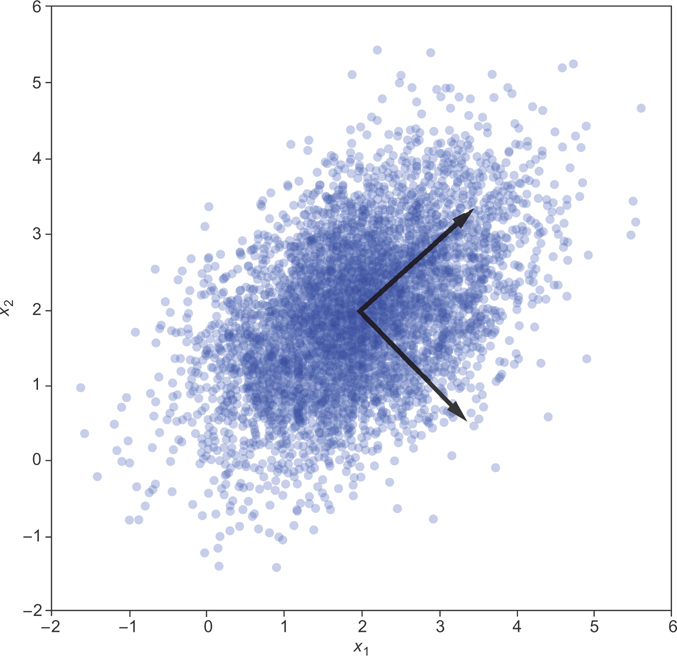
Figure 12.3 The two principal components of a 2-D gaussian data set
You can see that when you find zi by projecting the xi into these components, you should have no covariance. If you look at the original data, you find the covariance matrix in Figure 12.4. After transforming, you find the correlations in Figure 12.5.
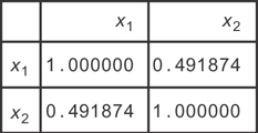
Figure 12.4 The correlation matrix for the xi
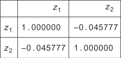
Figure 12.5 The correlation matrix for the zi
1 pd.DataFrame(model.transform(X), columns=['$z_1$', '$z_2$']).corr()
You can see that the correlations are now gone, so you’ve removed the collinearity in the data!
12.4.1 Complexity
The time complexity for PCA is O(min(N3, C3)) [27]. Assuming there are roughly as many samples as features, it’s just O(N2) [28, 29].
12.4.2 Memory Considerations
You should have enough memory available to factorize your CxN matrix and find the eigenvalue decomposition.
12.4.3 Tools
This is a widely implemented algorithm. sklearn makes an implementation available at sklearn.decomposition.PCA. You can also find PCA implemented in C++ by the mlpack library.
12.5 Independent Component Analysis
When a data set is produced by a number of independent sources all jumbled together, independent component analysis (ICA) offers a technique to separate them for analysis. The largest signals can then be modeled, ignoring smaller signals as noise. Similarly, if there is a great deal of noise superimposed on a small signal, they can be separated such that the small signal isn’t eclipsed.
ICA is a model that is similar to factor analysis. In this case, instead of using a Gaussian prior for the zi, you use any non-Gaussian prior. It turns out that factor analysis varies up to a rotation! If you want a unique set of factors, you have to choose a different prior.
Let’s apply this data to try to find the big five personality traits from some online data, at http://personality-testing.info/.
There are about 19,000 responses in this data to 50 questions. Each response is on a five-point scale. You can see the correlation matrix for this data in Figure 12.6. In this data, you’ll notice that there are blocks along the diagonal. This is a well-designed questionnaire, based on selecting and testing questions. The test was developed using factor analysis methods to find which questions gave the best measurements of the latent factors. These questions, the xi data, are then used to measure these factors, the zi data, which are interpreted as personality traits. The questions that measure each factor are given in Figures 12.7.
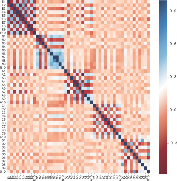
Figure 12.6 The correlation matrix for the big-five personality trait data. Notice the blocks of high and low covariance, forming checkered patterns.
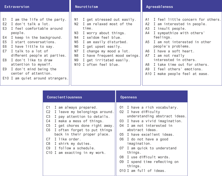
Figure 12.7 These are the questions underlying the big five personality traits. There are ten questions per trait, and they can correlate both positively and negatively with the underlying trait.
You can run the model on this data set, using sklearn’s FastICA implementation, which will generate Figure 12.8.
1 from sklearn.decomposition import FastICA
2 model = FastICA(n_components=5)
3 model = model.fit(X[questions])
4 heatmap(model.components_, cmap='RdBu')
You can see in Figure 12.8 that the factors are along the y-axis, and the questions are along the x-axis. When a question is relevant for a factor, the values for the factor loadings are either low or high.
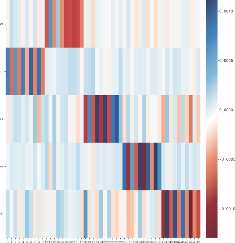
Figure 12.8 The matrix W for the big-five personality data
Finally, you can translate the sets of question responses into scores on the latent factors using the transformation in the model.
1 Z = model.transform(X[questions])
You can histogram the columns of the Z matrix and see the distributions of the individual’s scores (e.g., extraversion in Figure 12.9)!
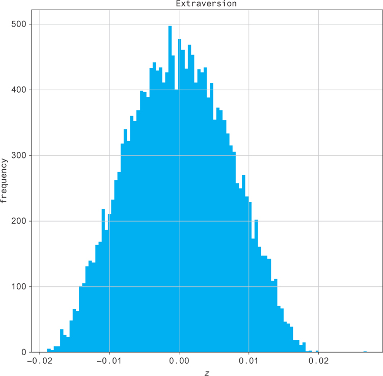
Figure 12.9 Distributions of the individual’s score
12.5.1 Assumptions
The main assumption of this technique is the independence of signal sources. Another important consideration is the desire to have as many mixtures as signals (not always totally necessary). Finally, a signal being extracted can’t be any more complex than the mixture it was extracted from (see, for example, pages 13–14 of [30]).
12.5.2 Complexity
There are fast algorithms for running ICA, including a fixed-point algorithm for FastICA [31] that runs quickly in practice, and a nonparametric kernel density estimation approach that runs in N log(N) time [32].
12.5.3 Memory Considerations
You should be able to fit at least C × N elements in memory.
12.5.4 Tools
ICA is another of those algorithms that seems to be implemented all over the place. FastICA is one of the more popular implementations. You can find it in scikit-learn as well as a C++ library implementing it. You’ll find even more at http://research.ics.aalto.fi/ica/fastica/.
12.6 Latent Dirichlet Allocation
Topic modeling, or latent dirichlet allocation, is a good illustration of the power of Bayesian methods. The problem is that you have a collection of text documents that you’d like to organize into categories but don’t have a good way to do it. There are too many documents to read all of them, but you’re fine putting them into an algorithm to do the work.
You distill down the documents into a bag-of-words representation and often just one part of speech (e.g., nouns). Different nouns are associated at different levels with the various topics. For example, “football” almost certainly is from a sports topic, while “yard” could be referring to distance gained in a game of football or to someone’s property. It might belong to both the “sports” and “homeowner” topics. Now, you just need a procedure to generate this text.
We’ll describe a process that will map to a graphical model. The process will generate these bags of words. Then, you can adjust the parameters describing the process to fit the data set, and discover the latent topics associated with our documents. First, we should define some terms. We need to formalize the concept of a topic.
We’ll describe a topic formally as a discrete probability distribution over our vocabulary. If you know a text is about one specific topic, the distribution will represent the word distribution of that document (although in practice, documents tend to be combinations of topics). In the sports topic, for example, you might find the word football occurring far more frequently than in other topics. It still might not be common, so it will have relatively low probability but will be much larger than it would be otherwise. In practice, sorting the words in a topic by their probability of being chosen is a good way to understand the topics you’ve discovered.
You also need a formal definition for a document. We mentioned that we’ll represent documents as bags of words. We’ll represent the topic membership of the document as a distribution over topics. If a document has a lot of weight on one topic, then any particular word from that document will likely be drawn from that topic. Now we’re ready to describe our generative process.
The process will go like this:
Draw the word distributions that define each topic.
Draw a topic distribution for each document.
For each word position in each document, draw a topic from the document’s topic distribution and then draw a word from the topic.
In that way, you generate the whole set of documents. With this process, you can fit your documents to discover the topic distributions for each document that generate the text, as well as the word distributions for those topics. First, you have to turn the whole process into a graphical model. To do that, you have to define priors as well, so you can draw the word distributions that define your topics, and we draw topic distributions that describe your documents.
Each of these distributions is categorical: it’s a normalized probability distribution over a collection of items (either topics or words). You need a probability distribution you can use to draw these distributions from! Let’s think of a simpler case first: a Bernoulli distribution, or unfair coin flip.
The parameter for the Bernoulli distribution is a probability of a success. What you want to do for your word distributions is draw a probability of choosing a word. You can think of it as a higher-dimensional coin flip. To draw the coin flip probability, you need a distribution whose domain is between zero and one, and the beta distribution is a good candidate.
The beta distribution has a higher-dimensional generalization: the dirichlet distribution. Each draw from a dirichlet distribution is a normalized vector of probabilities. You can choose the dirichlet distribution as the priors for our topic distributions (documents) and word distributions (topics).
Typically people will choose uniform priors for the dirichlet distributions and leave them with relatively high variance. That allows you to have unlikely words and topics but biases slightly toward everything being equally likely.
With the priors defined, you can formalize the process a little more. For M documents, N topics, and V words in the vocabulary, you can describe it as follows:
Draw a word distribution, ti (a topic), from Dir (α) for each i ∈ {1, . . . , N}.
Draw a topic distribution, dj (a document), from Dir(β) for each j ∈ {1, . . . , M}.
For the kth word position in document j, draw the topic t ∈ {1, . . . , N} from dj, and then the word from t.
It’s beyond our scope to go into detail for methods to fit LDA. You should check [33].
There are some important rules of thumb to get topic modeling to work well. We’ll summarize them as follows:
Tokenize, stem, and n-gram your text into bags of words.
Keep just the nouns from the text.
Remove any word that occurs fewer than five times.
Short documents (e.g., under ten words) will often have too large uncertainty for their topics to be useful.
Now, let’s check out gensim [34] to see how to fit a topic model! We’ll use the 20-newsgroups data set in sklearn as an example. We’ll use the nltk to do the stemming and part-of-speech tagging and otherwise use gensim to do the heavy lifting. You may need to download some models for nltk, and it will prompt you with error messages if you do.
First, let’s see what the part of speech tagger’s output looks like.
1 import nltk
2 phrase = "The quick gray fox jumps over the lazy dog"
3 text = nltk.word_tokenize(phrase)
4 nltk.pos_tag(text)
That produces the following output:
[('The', 'DT'),
 ('quick', 'JJ'),
 ('gray', 'JJ'),
 ('fox', 'NN'),
 ('jumps', 'NNS'),
 ('over', 'IN'),
 ('the', 'DT'),
 ('lazy', 'JJ'),
 ('dog', 'NN')]
You can look up parts of speech with queries like this:
nltk. help.upenn_tagset('NN')
NN: noun, common, singular or mass
    common-carrier cabbage knuckle-duster Casino afghan shed thermostat
    investment slide humour falloff slick wind hyena override subhumanity
    machinist ...
You want just the nouns, so we’ll keep the “NN” tags. Proper nouns have the “NNP” tag, and you’ll want those too. See the nltk documentation for a full listing of tags to see which others you might want to include. This code will do the trick:
1 desired_tags = ['NN', 'NNP']
2 nouns_only = []
3 for document in newsgroups_train['data']:
4     tokenized = nltk.word_tokenize(document)
5     tagged = nltk.pos_tag(tokenized)
6     nouns_only.append([word for word, tag in tagged
7                        if tag in desired_tags])
Now, you want to stem the words. You’ll use a language-specific stemmer, since those will do a better job.
1 from nltk.stem.snowball import SnowballStemmer
2
3 stemmer = SnowballStemmer("english")
4
5 for i, bag_of_words in enumerate(nouns_only):
6     for j, word in enumerate(bag_of_words):
7         nouns_only[i][j] = stemmer.stem(word)
Now, you want to count the words and make sure to keep words with only five or more occurrences.
1 word_counts = Counter()
2 for bag_of_words in nouns_only:
3     for word in bag_of_words:
4         word_counts[word] += 1
5
6 for i, bag_of_words in enumerate(nouns_only):
7     for word in enumerate(bag_of_words):
8         nouns_only[i] = [word for word in bag_of_words
9                          if word_counts[word] >= 5]
If you count the total words before and after stemming, you find 135,348 terms before and 110,858 after. You get rid of about 25,000 terms by stemming! Finally, you need to map your documents into the bag-of-words representation understood by gensim. It takes lists of (word, count) tuples, where the count is the number of times a word occurs in the document. To do this, you need the word to be an integer index corresponding to the word. You can make the word index mapping and use it when you create the tuples.
1 dictionary = {i: word for i, word in enumerate(word_counts.keys())}
2 word_index = {v:k for k, v in dictionary.items()}
3
4 for bag_of_words in enumerate(nouns_only):
5     counts = Counter(bag_of_words)
6     nouns_only[i] = [(word_index[word], count) for
7                       word, count in counts.items()]
Now, you can finally run the model. If you pass in the word mapping, there’s a nice method to print the top terms in the topics you’ve discovered.
1 from gensim import models
2
3 model = models.LdaModel(nouns_only,
4                         id2word=dictionary,
5                         num_topics=20)
6 model.show_topics()
That produces the output shown here:
 1 [(12,
 2   '0.031*"god" + 0.030*">" + 0.013*"jesus" + 0.010*"x" + 0.009*"@"
 3    + 0.008*"law" + 0.006*"encrypt" + 0.006*"time"
 4    + 0.006*"christian" + 0.006*"subject"'),
 5  (19,
 6   '0.011*"@" + 0.011*"stephanopoulo" + 0.010*"subject"
 7    + 0.009*"univers" + 0.008*"organ" + 0.005*"ripem"
 8    + 0.005*"inform" + 0.005*"greec" + 0.005*"church"
 9    + 0.005*"greek"'),
10  (16,
11   '0.022*"team" + 0.017*"@" + 0.016*"game" + 0.011*">"
12    + 0.010*"season" + 0.010*"hockey" + 0.009*"year" + 0.009*"subject"
13    + 0.009*"organ" + 0.008*"nhl"'),
14  (18,
15   '0.056*"@" + 0.045*">" + 0.016*"subject" + 0.015*"organ"
16    + 0.011*"re" + 0.009*"articl" + 0.007*"<" + 0.007*"univers"
17    + 0.006*"nntp-posting-host" + 0.004*"comput"'),
18  (1,
19   '0.075*"*" + 0.022*"@" + 0.016*"sale" + 0.013*"subject"
20    + 0.013*"organ" + 0.011*"univers" + 0.008*"nntp-posting-host"
21    + 0.006*"offer" + 0.005*"distribut" + 0.005*"tape"'),
22  (11,
23   '0.040*"q" + 0.021*"presid" + 0.014*"mr." + 0.006*"packag"
24    + 0.006*"event" + 0.006*">" + 0.005*"handler" + 0.005*"@"
25    + 0.004*"mack" + 0.004*"whaley"'),
26  (13,
27   '0.037*"@" + 0.020*"drive" + 0.018*"subject" + 0.017*"organ"
28    + 0.011*"card" + 0.010*"univers" + 0.010*"problem" + 0.009*"disk"
29    + 0.009*"system" + 0.008*"nntp-posting-host"'),
30  (6,
31   '0.065*">" + 0.055*"@" + 0.015*"organ" + 0.014*"subject"
32    + 0.013*"re" + 0.012*"articl" + 0.007*"|" + 0.006*"univers"
33    + 0.006*"<" + 0.006*"nntp-posting-host"'),
34  (7,
35   '0.053*">" + 0.039*"@" + 0.011*"subject" + 0.010*"organ"
36    + 0.010*"re" + 0.009*"articl" + 0.006*"univers" + 0.006*"]"
37    + 0.005*"<" + 0.004*"year"'),
38  (17,
39   '0.160*"|" + 0.028*"@" + 0.015*"subject" + 0.014*"organ"
40    + 0.013*"/" + 0.008*"\" + 0.008*"nntp-posting-host" + 0.008*">"
41    + 0.007*"+" + 0.007*"univers"')]
You can see a few things in these results. First, there is a lot of extra junk in the text that we haven’t filtered out yet. Before even tokenizing, you should use regex to replace the nonword characters, punctuation, and markup. You can also see some common terms like subject and nntp-posting-host that are likely to occur in any topic. These are frequent terms that we should really just filter out or use term weighting to suppress. Gensim has some nice tutorials on their website, and we recommend going there to see how to use term frequency, inverse document frequency (tfidf) weighting to suppress common terms without having to remove them from the data.
You can also see that there is something discovered in the data despite the noise. The first topic has god, jesus, and christian in the top terms so is likely corresponding to a religion news group. You could see which newsgroups weight highly on this topic to check for yourself.
A quick way to remove bad characters is to filter everything that isn’t a character or number using regular expressions. You can use the Python re package to do this, replacing with spaces. These will turn into nothing when they’re tokenized.
1 filtered = [re.sub('[^a-zA-Z0-9]+', ' ', document) for document
2             in newsgroups_train['data']]
If you run through the same procedure again after filtering, you get the following:
 1 [(3,
 2   '0.002*"polygon" + 0.002*"simm" + 0.002*"vram" + 0.002*"lc"
 3    + 0.001*"feustel" + 0.001*"dog" + 0.001*"coprocessor"
 4    + 0.001*"nick" + 0.001*"lafayett" + 0.001*"csiro"'),
 5  (9,
 6   '0.002*"serdar" + 0.002*"argic" + 0.001*"brandei"
 7    + 0.001*"turk" + 0.001*"he" + 0.001*"hab" + 0.001*"islam"
 8    + 0.001*"tyre" + 0.001*"zuma" + 0.001*"ge"'),
 9  (5,
10   '0.004*"msg" + 0.003*"god" + 0.002*"religion" + 0.002*"fbi"
11    + 0.002*"christian" + 0.002*"cult" + 0.002*"atheist"
12    + 0.002*"greec" + 0.001*"life" + 0.001*"robi"'),
13  (11,
14   '0.004*"pitt" + 0.004*"gordon" + 0.003*"bank"
15    + 0.002*"pittsburgh" + 0.002*"cadr" + 0.002*"geb"
16    + 0.002*"duo" + 0.001*"skeptic" + 0.001*"chastiti"
17    + 0.001*"talent"'),
18  (8,
19   '0.003*"access" + 0.003*"gun" + 0.002*"cs" + 0.002*"edu"
20    + 0.002*"x" + 0.002*"dos" + 0.002*"univers"
21    + 0.002*"colorado" + 0.002*"control" + 0.002*"printer"'),
22  (15,
23   '0.002*"athen" + 0.002*"georgia" + 0.002*"covington"
24    + 0.002*"drum" + 0.001*"aisun3" + 0.001*"rsa"
25    + 0.001*"arromde" + 0.001*"ai" + 0.001*"ham"
26    + 0.001*"missouri"'),
27  (16,
28   '0.002*"ranck" + 0.002*"magnus" + 0.002*"midi"
29    + 0.002*"alomar" + 0.002*"ohio" + 0.001*"skidmor"
30    + 0.001*"epa" + 0.001*"diablo" + 0.001*"viper"
31    + 0.001*"jbh55289"'),
32  (19,
33   '0.002*"islam" + 0.002*"stratus" + 0.002*"com"
34    + 0.002*"mot" + 0.002*"comet" + 0.001*"virginia"
35    + 0.001*"convex" + 0.001*"car" + 0.001*"jaeger"
36    + 0.001*"gov"'),
37  (0,
38   '0.005*"henri" + 0.003*"dyer" + 0.002*"zoo"
39    + 0.002*"spencer" + 0.002*"zoolog" + 0.002*"spdcc"
40    + 0.002*"prize" + 0.002*"outlet" + 0.001*"tempest"
41    + 0.001*"dresden"'),
42  (14,
43   '0.006*"god" + 0.005*"jesus" + 0.004*"church"
44    + 0.002*"christ" + 0.002*"sin" + 0.002*"bibl"
45    + 0.002*"templ" + 0.002*"mari" + 0.002*"cathol"
46    + 0.002*"jsc"')]
These results are pretty obviously better but still aren’t perfect. There are many parameters to tune with algorithms like these, so this should put you in a good place to start experimenting.
We should mention one powerful aspect of gensim. It operates on a generator for items, instead of a batch of items. That allows you to work with very large data sets without having to load them into memory. Gensim is appropriate for, as their tutorial suggests, modeling the topics within Wikipedia and other large corpuses.
12.7 Conclusion
In this chapter, you saw how to use some Bayesian network and other methods to reduce the dimension of data and discover latent structure in the data. We walked through some examples that are useful for analyzing survey response and other categorical data. We went through a detailed example to learn topic modeling. Ideally now you’re familiar with latent variable models enough to be able to use them confidently!