Chapter 1. A machine-learning odyssey

This chapter covers

• Machine-learning fundamentals
• Data representation, features, and vector norms
• Why TensorFlow

Have you ever wondered if there are limits to what computer programs can solve? Nowadays, computers appear to do a lot more than unravel mathematical equations. In the last half-century, programming has become the ultimate tool to automate tasks and save time, but how much can we automate, and how do we go about doing so?

Can a computer observe a photograph and say, “Aha, I see a lovely couple walking over a bridge under an umbrella in the rain”? Can software make medical decisions as accurately as trained professionals can? Can software predictions about the stock market perform better than human reasoning? The achievements of the past decade hint that the answer to all these questions is a resounding yes, and the implementations appear to share a common strategy.

Recent theoretical advances coupled with newly available technologies have enabled anyone with access to a computer to attempt their own approach at solving these incredibly hard problems. Okay, not just anyone, but that’s why you’re reading this book, right?

A programmer no longer needs to know the intricate details of a problem to solve it. Consider converting speech to text: a traditional approach may involve understanding the biological structure of human vocal chords to decipher utterances by using many hand-designed, domain-specific, un-generalizable pieces of code. Nowadays, it’s possible to write code that looks at many examples and figures out how to solve the problem, given enough time and examples.

Algorithms learn from data, similar to the way humans learn from experience. Humans learn by reading books, observing situations, studying in school, exchanging conversations, and browsing websites, among other means. How can a machine possibly develop a brain capable of learning? There’s no definitive answer, but world-class researchers have developed intelligent programs from different angles. Among the implementations, scholars have noticed recurring patterns in solving these kinds of problems that has led to a standardized field that we today label machine learning (ML).

As the study of ML matures, the tools have become more standardized, robust, high-performing, and scalable. This is where TensorFlow comes in. This software library has an intuitive interface that lets programmers dive into using complex ML ideas. The next chapter presents the ins and outs of this library, and every chapter thereafter explains how to use TensorFlow for each of the various ML applications.

1.1. Machine-learning fundamentals

Have you ever tried to explain to someone how to swim? Describing the rhythmic joint movements and fluid patterns is overwhelming in its complexity. Similarly, some software problems are too complicated for us to easily wrap our minds around. For this, machine learning may be just the tool to use.

Handcrafting carefully tuned algorithms to get the job done was once the only way of building software. From a simplistic point of view, traditional programming assumes a deterministic output for each input. Machine learning, on the other hand, can solve a class of problems for which the input-output correspondences aren’t well understood.

Machine learning is characterized by software that learns from previous experiences. Such a computer program improves performance as more and more examples are available. The hope is that if you throw enough data at this machinery, it’ll learn patterns and produce intelligent results for newly fed input.

Another name for machine learning is inductive learning, because the code is trying to infer structure from data alone. It’s like going on vacation in a foreign country, and reading a local fashion magazine to mimic how to dress. You can develop an idea of the culture from images of people wearing local articles of clothing. You’re learning inductively.

You might never before have used such an approach when programming, because inductive learning isn’t always necessary. Consider the task of determining whether the sum of two arbitrary numbers is even or odd. Sure, you can imagine training a machine-learning algorithm with millions of training examples (outlined in figure 1.1), but you certainly know that’s overkill. A more direct approach can easily do the trick.

Figure 1.1. Each pair of integers, when summed, results in an even or odd number. The input and output correspondences listed are called the ground-truth dataset.

For example, the sum of two odd numbers is always an even number. Convince yourself: take any two odd numbers, add them, and check whether the sum is an even number. Here’s how you can prove that fact directly:

• For any integer n, the formula 2n + 1 produces an odd number. Moreover, any odd number can be written as 2n + 1 for some value n. The number 3 can be written as 2(1) + 1. And the number 5 can be written as 2(2) + 1.
• Let’s say we have two odd numbers, 2n + 1 and 2m + 1, where n and m are integers. Adding two odd numbers yields (2n + 1) + (2m + 1) = 2n + 2m + 2 = 2(n + m + 1). This is an even number because 2 times anything is even.

Likewise, we see that the sum of two even numbers is also an even number: 2m + 2n = 2(m + n). And lastly, we also deduce that the sum of an even with an odd is an odd number: 2m + (2n + 1) = 2(m + n) + 1. Figure 1.2 presents this logic more clearly.

Figure 1.2. This table reveals the inner logic behind how the output response corresponds to the input pairs.

That’s it! With absolutely no use of machine learning, you can solve this task on any pair of integers someone throws at you. Directly applying mathematical rules can solve this problem. But in ML algorithms, we can treat the inner logic as a black box, meaning the logic happening inside might not be obvious to interpret, as depicted in figure 1.3.

Figure 1.3. An ML approach to solving problems can be thought of as tuning the parameters of a black box until it produces satisfactory results.

1.1.1. Parameters

Sometimes, the best way to devise an algorithm that transforms an input to its corresponding output is too complicated. For example, if the input were a series of numbers representing a grayscale image, you can imagine the difficulty in writing an algorithm to label every object in the image. Machine learning comes in handy when the inner workings aren’t well understood. It provides us with a toolset to write software without defining every detail of the algorithm. The programmer can leave some values undecided and let the machine-learning system figure out the best values by itself.

The undecided values are called parameters, and the description is referred to as the model. Your job is to write an algorithm that observes existing examples to figure out how to best tune parameters to achieve the best model. Wow, that’s a mouthful! Don’t worry, this concept will be a reoccurring motif.

1.1.2. Learning and inference

Suppose you’re trying to bake desserts in an oven. If you’re new to the kitchen, it can take days to come up with both the right combination and perfect ratio of ingredients to make something that tastes great. By recording recipes, you can remember how to quickly repeat the dessert if you happen to discover the ultimate tasty meal.

Similarly, machine learning shares this idea of recipes. Typically, we examine an algorithm in two stages: learning and inference. The objective of the learning stage is to describe the data, which is called the feature vector, and summarize it in a model. The model is our recipe. In effect, the model is a program with a couple of open interpretations, and the data helps disambiguate it.

Note

A feature vector is a practical simplification of data. You can think of it as a sufficient summary of real-world objects into a list of attributes. The learning and inference steps rely on the feature vector instead of the data directly.

Similar to the way recipes can be shared and used by other people, the learned model is reused by other software. The learning stage is the most time consuming. Running an algorithm may take hours, if not days or weeks, to converge into a useful model. Figure 1.4 outlines the learning pipeline.

Figure 1.4. The learning approach generally follows a structured recipe. First, the dataset needs to be transformed into a representation, most often a list of features, which can be used by the learning algorithm. The learning algorithm chooses a model and efficiently searches for the model’s parameters.

The inference stage uses the model to make intelligent remarks about never-before-seen data. It’s like using a recipe you found online. The process of inference typically takes orders of magnitude less time than learning; inference can be fast enough to work on real-time data. Inference is all about testing the model on new data and observing performance in the process, as shown in figure 1.5.

Figure 1.5. The inference approach generally uses a model that has already been either learned or given. After converting data into a usable representation, such as a feature vector, it uses the model to produce intended output.

1.2. Data representation and features

Data is a first-class citizen of machine learning. Computers are nothing more than sophisticated calculators, and so the data we feed our machine-learning systems must be mathematical objects such as vectors, matrices, or graphs.

The basic theme in all forms of representation is the concept of features, which are observable properties of an object:

• Vectors have a flat and simple structure and are the typical embodiment of data in most real-world machine-learning applications. They have two attributes: a natural number representing the dimension of the vector, and a type (such as real numbers, integers, and so on). Just as a refresher, some examples of two-dimensional vectors of integers are (1, 2) and (–6, 0). Some examples of three-dimensional vectors of real numbers are (1.1, 2.0, 3.9) and (Π, Π/2, Π/3). You get the idea: a collection of numbers of the same type. In a program that uses machine learning, a vector measures a property of the data, such as color, density, loudness, or proximity—anything you can describe with a series of numbers, one for each thing being measured.
• Moreover, a vector of vectors is a matrix. If each feature vector describes the features of one object in your dataset, the matrix describes all the objects; each item in the outer vector is a node that’s a list of features of one object.
• Graphs, on the other hand, are more expressive. A graph is a collection of objects (nodes) that can be linked together with edges to represent a network. A graphical structure enables representing relationships between objects, such as in a friendship network or a navigation route of a subway system. Consequently, they’re tremendously harder to manage in machine-learning applications. In this book, our input data will rarely involve a graphical structure.

Feature vectors are practical simplifications of real-world data, which can be too complicated to deal with. Instead of attending to every little detail of a data item, a feature vector is a practical simplification. For example, a car in the real world is much more than the text used to describe it. A car salesman is trying to sell you the car, not the intangible words spoken or written. Those words are just abstract concepts, similar to the way feature vectors are just summaries of the data.

The following scenario will explain this further. When you’re in the market for a new car, keeping tabs on every minor detail of different makes and models is essential. After all, if you’re about to spend thousands of dollars, you may as well do so diligently. You’d likely record a list of features about each car and compare them back and forth. This ordered list of features is the feature vector.

When shopping for cars, you might find comparing mileage to be more lucrative than comparing something less relevant to your interest, such as weight. The number of features to track also must be just right: not too few, or you’ll lose information you care about, and not too many, or they’ll be unwieldy and time consuming to keep track of. This tremendous effort to select both the number of measurements and which measurements to compare is called feature engineering. Depending on which features you examine, the performance of your system can fluctuate dramatically. Selecting the right features to track can make up for a weak learning algorithm.

For example, when training a model to detect cars in an image, you’ll gain an enormous performance and speed improvement if you first convert the image to grayscale. By providing some of your own bias when preprocessing the data, you end up helping the algorithm, because it won’t need to learn that colors don’t matter when detecting cars. The algorithm can instead focus on identifying shapes and textures, which will lead to much faster learning than trying to process colors as well.

The general rule of thumb in ML is that more data produces better results. But the same isn’t always true of having more features. Perhaps counterintuitively, if the number of features you’re tracking is too high, performance may suffer. Populating the space of all data with representative samples requires exponentially more data as the dimension of the feature vector increases. As a result, feature engineering, as depicted in figure 1.6, is one of the most significant problems in ML.

Figure 1.6. Feature engineering is the process of selecting relevant features for the task.

You may not appreciate it right away, but something consequential happens when you decide which features are worth observing. For centuries, philosophers have pondered the meaning of identity; you may not immediately realize this, but you’ve come up with a definition of identity by your choice of specific features.

Imagine writing a machine-learning system to detect faces in an image. Let’s say one of the necessary features for something to be a face is the presence of two eyes. Implicitly, a face is now defined as something with eyes. Do you realize the kind of trouble this can get you into? If a photo of a person shows them blinking, your detector won’t find a face, because it can’t find two eyes. The algorithm would fail to detect a face when a person is blinking. The definition of a face was inaccurate to begin with, and it’s apparent from the poor detection results.

The identity of an object is decomposed into the features from which it’s composed. For example, if the features you’re tracking of one car exactly match the corresponding features of another car, they may as well be indistinguishable from your perspective. You’d need to add another feature to the system in order to tell them apart, or you’ll think they’re the same item. When handcrafting features, you must take great care not to fall into this philosophical predicament of identity.

Feature engineering is a refreshingly philosophical pursuit. For those who enjoy thought-provoking escapades into the meaning of self, we invite you to meditate on feature selection, because it’s still an open problem. Fortunately for the rest of you, to alleviate extensive debates, recent advances have made it possible to automatically determine which features to track. You’ll be able to try it out for yourself in chapter 7.

1.3. Distance metrics

If you have feature vectors of cars you may potentially want to buy, you can figure out which two are most similar by defining a distance function on the feature vectors. Comparing similarities between objects is an essential component of machine learning. Feature vectors allow us to represent objects so that we may compare them in a variety of ways. A standard approach is to use the Euclidian distance, which is the geometric interpretation you may find most intuitive when thinking about points in space.

Let’s say we have two feature vectors, x = (x₁, x₂, ..., x_n) and y = (y₁, y₂, ..., y_n). The Euclidian distance ||x – y|| is calculated by

For example, the Euclidian distance between (0, 1) and (1, 0) is

Scholars call this the L2 norm. But that’s just one of many possible distance functions. The L0, L1, and L-infinity norms also exist. All these norms are valid ways to measure distance. Here they are in more detail:

• The L0 norm counts the total number of nonzero elements of a vector. For example, the distance between the origin (0, 0) and vector (0, 5) is 1, because there’s only one nonzero element. The L0 distance between (1, 1) and (2, 2) is 2, because neither dimension matches up. Imagine that the first and second dimensions represent username and password, respectively. If the L0 distance between a login attempt and the true credentials is 0, the login is successful. If the distance is 1, then either the username or password is incorrect, but not both. Lastly, if the distance is 2, both username and password aren’t found in the database.
• The L1 norm, shown in figure 1.7, is defined as Σ|x_n|. The distance between two vectors under the L1 norm is also referred to as the Manhattan distance. Imagine living in a downtown area like Manhattan, New York, where the streets form a grid. The shortest distance from one intersection to another is along the blocks. Similarly, the L1 distance between two vectors is along the orthogonal directions. The distance between (0, 1) and (1, 0) under the L1 norm is 2. Computing the L1 distance between two vectors is the sum of absolute differences at each dimension, which is a useful measure of similarity.

  Figure 1.7. The L1 distance is also called the Manhattan distance (also referred to as the taxicab metric), because it resembles the route of a car in a grid-like neighborhood such as Manhattan. If a car is traveling from point (0,1) to point (1,0), the shortest route requires a length of 2 units.

  

• The L2 norm, shown in figure 1.8, is the Euclidian length of a vector, (Σ(x_n)²)^1/2. It’s the most direct route you can possibly take on a geometric plane to get from one point to another. For the mathematically inclined, this is the norm that implements the least square estimation as predicted by the Gauss-Markov theorem. For the rest of you, it’s the shortest distance between two points in space.

  Figure 1.8. The L2 norm between points (0,1) and (1,0) is the length of a single straight-line segment between both points.

  

• The L-N norm generalizes this pattern, resulting in (Σ|x_n|^N)^1/N. We rarely use finite norms above L2, but it’s here for completeness.
• The L-infinity norm is (Σ|x_n|^∞)^1/∞. More naturally, it’s the largest magnitude among each element. If the vector is (–1, –2, –3), the L-infinity norm is 3. If a feature vector represents costs of various items, minimizing the L-infinity norm of the vector is an attempt to reduce the cost of the most expensive item.

1.4. Types of learning

Now that you can compare feature vectors, you have the tools necessary to use data for practical algorithms. Machine learning is often split into three perspectives: supervised learning, unsupervised learning, and reinforcement learning. Let’s examine each.

1.4.1. Supervised learning

By definition, a supervisor is someone higher up in the chain of command. When we’re in doubt, our supervisor dictates what to do. Likewise, supervised learning is all about learning from examples laid out by a supervisor (such as a teacher).

A supervised machine-learning system needs labeled data to develop a useful understanding, which we call its model. For example, given many photographs of people and their recorded corresponding ethnicity, we can train a model to classify the ethnicity of a never-before-seen individual in an arbitrary photograph. Simply put, a model is a function that assigns a label to data. It does so by using a collection of previous examples, called a training dataset, as reference.

A convenient way to talk about models is through mathematical notation. Let x be an instance of data, such as a feature vector. The corresponding label associated with x is f(x), often referred to as the ground truth of x. Usually, we use the variable y = f(x) because it’s quicker to write. In the example of classifying the ethnicity of a person through a photograph, x can be a 100-dimensional vector of various relevant features, and y is one of a couple of values to represent the various ethnicities. Because y is discrete with few values, the model is called a classifier. If y can result in many values, and the values have a natural ordering, then the model is called a regressor.

Let’s denote a model’s prediction of x as g(x). Sometimes you can tweak a model to change its performance drastically. Models have parameters that can be tuned either by a human or automatically. We use the vector θ to represent the parameters. Putting it all together, g(x|θ) more completely represents the model, read “g of x given θ.”

Note

Models may also have hyperparameters, which are extra ad hoc properties about a model. The term hyper in hyperparameter seems a bit strange at first. If it helps, a better name could be metaparameter, because the parameter is akin to metadata about the model.

The success of a model’s prediction g(x|θ) depends on how well it agrees with the ground truth y. We need a way to measure the distance between these two vectors. For example, the L2 norm may be used to measure how close two vectors lie. The distance between the ground truth and the prediction is called the cost.

The essence of a supervised machine-learning algorithm is to figure out the parameters of a model that result in the least cost. Mathematically put, we’re looking for a θ* (Theta star) that minimizes the cost among all data points x ∈ X. One way of formalizing this optimization problem is the following:

Clearly, brute forcing every possible combination of θs (also known as a parameter space) will eventually find the optimal solution, but at an unacceptable runtime. A major area of research in machine learning is about writing algorithms that efficiently search through this parameter space. Some of the early algorithms include gradient descent, simulated annealing, and genetic algorithms. TensorFlow automatically takes care of the low-level implementation details of these algorithms, so we won’t get into them in too much detail.

After the parameters are learned one way or another, you can finally evaluate the model to figure out how well the system captured patterns from the data. A rule of thumb is to not evaluate your model on the same data you used to train it, because you already know it works for the training data; you need to tell whether it works for data that wasn’t part of the training set, to make sure your model is general purpose and not biased to the data used to train it. Use the majority of the data for training, and the remaining for testing. For example, if you have 100 labeled data points, randomly select 70 of them to train a model, and reserve the other 30 to test it.

1.4.2. Unsupervised learning

Unsupervised learning is about modeling data that comes without corresponding labels or responses. The fact that we can make any conclusions at all on raw data feels like magic. With enough data, it may be possible to find patterns and structure. Two of the most powerful tools that machine-learning practitioners use to learn from data alone are clustering and dimensionality reduction.

Clustering is the process of splitting the data into individual buckets of similar items. In a sense, clustering is like classification of data without knowing any corresponding labels. For instance, when organizing your books on three shelves, you likely place similar genres together, or maybe you group them by the authors’ last names. You might have a Stephen King section, another for textbooks, and a third for “anything else.” You don’t care that they’re all separated by the same feature, just that each has something unique about it that allows you to break it into roughly equal, easily identifiable groups. One of the most popular clustering algorithms is k-means, which is a specific instance of a more powerful technique called the E-M algorithm.

Dimensionality reduction is about manipulating the data to view it under a much simpler perspective. It’s the ML equivalent of the phrase, “Keep it simple, stupid.” For example, by getting rid of redundant features, we can explain the same data in a lower-dimensional space and see which features matter. This simplification also helps in data visualization or preprocessing for performance efficiency. One of the earliest algorithms is principle component analysis (PCA), and a newer one is autoencoders, which we cover in chapter 7.

1.4.3. Reinforcement learning

Supervised and unsupervised learning seem to suggest that the existence of a teacher is all or nothing. But in one well-studied branch of machine learning, the environment acts as a teacher, providing hints as opposed to definite answers. The learning system receives feedback on its actions, with no concrete promise that it’s progressing in the right direction, which might be to solve a maze or accomplish an explicit goal.

Unlike supervised learning, where training data is conveniently labeled by a “teacher,” reinforcement learning trains on information gathered by observing how the environment reacts to actions. Reinforcement learning is a type of machine learning that interacts with the environment to learn which combination of actions yields the most favorable results. Because we’re already anthropomorphizing algorithms by using the words environment and action, scholars typically refer to the system as an autonomous agent. Therefore, this type of machine learning naturally manifests itself in the domain of robotics.

To reason about agents in the environment, we introduce two new concepts: states and actions. The status of the world frozen at a particular time is called a state. An agent may perform one of many actions to change the current state. To drive an agent to perform actions, each state yields a corresponding reward. An agent eventually discovers the expected total reward of each state, called the value of a state.

Like any other machine-learning system, performance improves with more data. In this case, the data is a history of previous experiences. In reinforcement learning, we don’t know the final cost or reward of a series of actions until it’s executed. These situations render traditional supervised learning ineffective, because we don’t know exactly which action in the history of action sequences is to blame for ending up in a low-value state. The only information an agent knows for certain is the cost of a series of actions that it has already taken, which is incomplete. The agent’s goal is to find a sequence of actions that maximizes rewards.

1.5. TensorFlow

Google open-sourced its machine-learning framework, TensorFlow, in late 2015 under the Apache 2.0 license. Before that, it was used proprietarily by Google in its speech recognition, Search, Photos, and Gmail, among other applications.

The library is implemented in C++ and has a convenient Python API, as well as a lesser appreciated C++ API. Because of the simpler dependencies, TensorFlow can be quickly deployed to various architectures.

Similar to Theano (a popular numerical computation library for Python you may already be familiar with), computations are described as flowcharts, separating design from implementation. With little-to-no hassle, this dichotomy allows the same design to be implemented on not just large-scale training systems with thousands of processors, but also mobile devices. The single system spans a broad range of platforms.

One of the fanciest properties of TensorFlow is its automatic differentiation capabilities. You can experiment with new networks without having to redefine many key calculations.

Note

Automatic differentiation makes it much easier to implement back-propagation, which is a computationally heavy calculation used in a branch of machine learning called neural networks. TensorFlow hides the nitty-gritty details of back-propagation so you can focus on the bigger picture. Chapter 7 covers an introduction to neural networks with TensorFlow.

All the mathematics is abstracted away and unfolded under the hood. It’s like using WolframAlpha for a calculus problem set.

Another feature of this library is its interactive visualization environment called TensorBoard. This tool shows a flowchart of the way data transforms, displays summary logs over time, and traces performance. Figure 1.9 shows an example of what TensorBoard looks like when in use. The next chapter covers using it in greater detail.

Figure 1.9. Example of TensorBoard in action

Prototyping in TensorFlow is much faster than in Theano (code initiates in a matter of seconds as opposed to minutes) because many of the operations come precompiled. It becomes easy to debug code due to subgraph execution; an entire segment of computation can be reused without recalculation.

Because TensorFlow isn’t only about neural networks, it also has out-of-the-box matrix computation and manipulation tools. Most libraries such as Torch and Caffe are designed solely for deep neural networks, but TensorFlow is more flexible as well as scalable.

The library is well documented and officially supported by Google. Machine learning is a sophisticated topic, so having an exceptionally well-reputed company behind TensorFlow is comforting.

1.6. Overview of future chapters

Chapter 2 demonstrates how to use various components of TensorFlow (see figure 1.10). Chapters 3–6 show how to implement classic machine-learning algorithms in TensorFlow, and chapters 7–12 cover algorithms based on neural networks. The algorithms solve a wide variety of problems such as prediction, classification, clustering, dimensionality reduction, and planning.

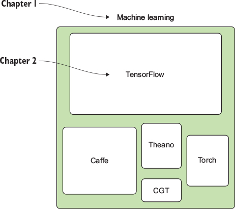
Figure 1.10. This chapter introduced fundamental machine-learning concepts, and the next chapter begins your journey into TensorFlow. Other tools to apply machine-learning algorithms (such as Caffe, Theano, and Torch) are available, but you’ll see in chapter 2 why TensorFlow is the way to go.

Many algorithms can solve the same real-world problem, and many real-world problems can be solved by the same algorithm. Table 1.1 covers the ones laid out in this book.

Table 1.1. Many real-world problems can be solved using the corresponding algorithm found in its respective chapter.

Real-world problem	Algorithm	Chapter
Predicting trends, fitting a curve to data points, describing relationships between variables	Linear regression	3
Classifying data into two categories, finding the best way to split a dataset	Logistic regression	4
Classifying data into multiple categories	Softmax regression	4
Revealing hidden causes of observations, finding the most likely hidden reason for a series of outcomes	Hidden Markov model (Viterbi)	5
Clustering data into a fixed number of categories, automatically partitioning data points into separate classes	K-means	6
Clustering data into arbitrary categories, visualizing high-dimensional data into a lower-dimensional embedding	Self-organizing map	6
Reducing dimensionality of data, learning latent variables responsible for high-dimensional data	Autoencoder	7
Planning actions in an environment using neural networks (reinforcement learning)	Q-policy neural network	8
Classifying data using supervised neural networks	Perceptron	9
Classifying real-world images using supervised neural networks	Convolution neural network	9
Producing patterns that match observations using neural networks	Recurrent neural network	10
Predicting natural language responses to natural language queries	Seq2seq model	11
Learning to rank items by learning their utility	Ranking	12

Tip

If you’re interested in the intricate architecture details of TensorFlow, the best available source is the official documentation at www.tensorflow.org/extend/architecture. This book will sprint ahead and use TensorFlow without slowing down for the breadth of low-level performance tuning. For those interested in cloud services, you may consider Google’s solution for professional-grade scale and speed: https://cloud.google.com/products/machine-learning/.

1.7. Summary

• TensorFlow has become the tool of choice among professionals and researchers to implement machine-learning solutions.
• Machine learning uses examples to develop an expert system that can make useful statements about new inputs.
• A key property of ML is that performance tends to improve with more training data.
• Over the years, scholars have crafted three major archetypes that most problems fit: supervised learning, unsupervised learning, and reinforcement learning.
• After a real-world problem is formulated in a machine-learning perspective, several algorithms become available. Out of the many software libraries and frameworks to accomplish an implementation, we chose TensorFlow as our silver bullet. Developed by Google and supported by its flourishing community, Tensor-Flow gives us a way to easily implement industry-standard code.