
Chapter 10. Recurrent neural networks

- Understanding the components of a recurrent neural network
- Designing a predictive model of time-series data
- Using the time-series predictor on real-world data
10.1. Contextual information
Back in school, I remember my sigh of relief when one of my midterm exams consisted of only true-or-false questions. I can’t be the only one who assumed that half the answers would be True and the other half would be False.
I figured out answers to most of the questions and left the rest to random guessing. But that guessing was based on something clever, a strategy that you might have employed as well. After counting my number of True answers, I realized that a disproportionate number of False answers were lacking. So, a majority of my guesses were False to balance the distribution.
It worked. I sure felt sly in the moment. What exactly is this feeling of craftiness that makes us feel so confident in our decisions, and how can we give a neural network the same power?
One answer is to use context to answer questions. Contextual cues are important signals that can improve the performance of machine-learning algorithms. For example, imagine you want to examine an English sentence and tag the part of speech of each word.
The naïve approach is to individually classify each word as a noun, an adjective, and so on, without acknowledging its neighboring words. Consider trying that technique on the words in this sentence. The word trying is used as a verb, but depending on the context, you can also use it as an adjective, making parts-of-speech tagging a trying problem.
A better approach considers the context. To bestow neural networks with contextual cues, you’ll study an architecture called a recurrent neural network. Instead of natural language data, you’ll be dealing with continuous time-series data, such as the stock market prices covered in previous chapters. By the end of the chapter, you’ll be able to model the patterns in time-series data to predict future values.
10.2. Introduction to recurrent neural networks
To understand recurrent neural networks, let’s first look at the simple architecture in figure 10.1. It takes as input a vector X(t) and generates as output a vector Y(t), at some time (t). The circle in the middle represents the hidden layer of the network.
Figure 10.1. A neural network with the input and output layers labeled as X(t) and Y(t), respectively
![]()
With enough input/output examples, you can learn the parameters of the network in TensorFlow. For instance, let’s refer to the input weights as a matrix Win and the output weights as a matrix Wout. Assume there’s just one hidden layer, referred to as a vector Z(t).
As shown in figure 10.2, the first half of the neural network is characterized by the function Z(t) = X(t) × Win, and the second half of the neural network takes the form Y(t) = Z(t) × Wout. Equivalently, if you prefer, the whole neural network is the function Y(t) = (X(t) × Win) × Wout.
Figure 10.2. The hidden layer of a neural network can be thought of as a hidden representation of the data, which is encoded by the input weights and decoded by the output weights.

After spending nights fine-tuning the network, you probably want to start using your learned model in a real-world scenario. Typically, that implies calling the model multiple times, maybe even repeatedly, as depicted in figure 10.3.
Figure 10.3. Often you end up running the same neural network multiple times, without using knowledge about the hidden states of the previous runs.

At each time t, when calling the learned model, this architecture doesn’t take into account knowledge about the previous runs. It’s like predicting stock market trends by looking only at data from the current day. A better idea is to exploit overarching patterns from a week’s worth or a month’s worth of data.
A recurrent neural network (RNN) is different from a traditional neural network because it introduces a transition weight W to transfer information over time. Figure 10.4 shows the three weight matrices that must be learned in an RNN. The introduction of the transition weight means that the next state is now dependent on the previous model, as well as the previous state. This means your model now has a “memory” of what it did!
Figure 10.4. A recurrent neural network architecture can use the previous states of the network to its advantage.

Diagrams are nice, but you’re here to get your hands dirty. Let’s get right to it! The next section shows how to use TensorFlow’s built-in RNN models. Then, you’ll use an RNN on real-world time-series data to predict the future!
10.3. Implementing a recurrent neural network
As you implement the RNN, you’ll use TensorFlow to do much of the heavy lifting. You won’t need to manually build up a network as shown earlier in figure 10.4, because the TensorFlow library already supports some robust RNN models.
Note
For TensorFlow library information on RNNs, see www.tensorflow.org/tutorials/recurrent.
One type of RNN model is called Long Short-Term Memory (LSTM). I admit, it’s a fun name. It means exactly what it sounds like, too: short-term patterns aren’t forgotten in the long term.
The precise implementation details of LSTM are beyond the scope of this book. Trust me, a thorough inspection of the LSTM model would distract from the chapter, because there’s no definite standard yet. That’s where TensorFlow comes to the rescue. It takes care of how the model is defined so you can use it out of the box. It also means that as TensorFlow is updated in the future, you’ll be able to take advantage of improvements to the LSTM model without modifying your code.
Tip
To understand how to implement LSTM from scratch, I suggest the following explanation: https://apaszke.github.io/lstm-explained.html. The paper that describes the implementation of regularization used in the following listings is available at http://arxiv.org/abs/1409.2329.
Begin by writing your code in a new file called simple_regression.py. Import the relevant libraries, as shown in the following listing.
Listing 10.1. Importing relevant libraries
import numpy as np
import tensorflow as tf
from tensorflow.contrib import rnn
Now, define a class called SeriesPredictor. The constructor, shown in the following listing, will set up model hyperparameters, weights, and the cost function.
Listing 10.2. Defining a class and its constructor
class SeriesPredictor:
    def __init__(self, input_dim, seq_size, hidden_dim=10):

        self.input_dim = input_dim                                        1
        self.seq_size = seq_size                                          1
        self.hidden_dim = hidden_dim                                      1

        self.W_out = tf.Variable(tf.random_normal([hidden_dim, 1]),       2
          name='W_out')                                                   2
        self.b_out = tf.Variable(tf.random_normal([1]), name='b_out')     2
        self.x = tf.placeholder(tf.float32, [None, seq_size, input_dim])  2
        self.y = tf.placeholder(tf.float32, [None, seq_size])             2

        self.cost = tf.reduce_mean(tf.square(self.model() - self.y))      3
        self.train_op = tf.train.AdamOptimizer().minimize(self.cost)      3

        self.saver = tf.train.Saver()                                     4
- 1 Hyperparameters
- 2 Weight variables and input placeholders
- 3 Cost optimizer
- 4 Auxiliary ops
Next, let’s use TensorFlow’s built-in RNN model called BasicLSTMCell. The hidden dimension of the cell passed into the BasicLSTMCell object is the dimension of the hidden state that gets passed through time. You can run this cell with data by using the rnn.dynamic_rnn function, to retrieve the output results. The following listing details how to use TensorFlow to implement a predictive model using LSTM.
Listing 10.3. Defining the RNN model
    def model(self):
        """
        :param x: inputs of size [T, batch_size, input_size]
        :param W: matrix of fully-connected output layer weights
        :param b: vector of fully-connected output layer biases
        """
        cell = rnn.BasicLSTMCell(self.hidden_dim)                                1
        outputs, states = tf.nn.dynamic_rnn(cell, self.x, dtype=tf.float32)      2
        num_examples = tf.shape(self.x)[0]
        W_repeated = tf.tile(tf.expand_dims(self.W_out, 0), [num_examples, 1, 1])3
        out = tf.matmul(outputs, W_repeated) + self.b_out
        out = tf.squeeze(out)
        return out
- 1 Creates an LSTM cell
- 2 Runs the cell on the input to obtain tensors for outputs and states
- 3 Computes the output layer as a fully connected linear function
With a model and cost function defined, you can now implement the training function, which will learn the LSTM weights, given example input/output pairs. As listing 10.4 shows, you open a session and repeatedly run the optimizer on the training data.
Note
You can use cross-validation to figure out how many iterations you need to train the model. In this case, you assume a fixed number of epochs. Some good insights and answers can be found through online Q&A sites such as ResearchGate: http://mng.bz/lB92.
After training, save the model to a file so you can load it later.
Listing 10.4. Training the model on a dataset
    def train(self, train_x, train_y):
        with tf.Session() as sess:
            tf.get_variable_scope().reuse_variables()
            sess.run(tf.global_variables_initializer())
            for i in range(1000):                                     1
                _, mse = sess.run([self.train_op, self.cost],
     feed_dict={self.x: train_x, self.y: train_y})
                if i % 100 == 0:
                    print(i, mse)
            save_path = self.saver.save(sess, 'model.ckpt')
            print('Model saved to {}'.format(save_path))
- 1 Runs the train op 1,000 times
Let’s say all went well, and your model has successfully learned parameters. Next, you’d like to evaluate the predictive model on other data. The following listing loads the saved model and runs the model in a session by feeding in test data. If a learned model doesn’t perform well on testing data, you can try tweaking the number of hidden dimensions of the LSTM cell.
Listing 10.5. Testing the learned model
    def test(self, test_x):
        with tf.Session() as sess:
            tf.get_variable_scope().reuse_variables()
            self.saver.restore(sess, './model.ckpt')
            output = sess.run(self.model(), feed_dict={self.x: test_x})
            print(output)
It’s done! But just to convince yourself that it works, let’s make up some data and try to train the predictive model. In the next listing, you’ll create input sequences, train_x, and corresponding output sequences, train_y.
Listing 10.6. Training and testing on dummy data
if __name__ == '__main__':
    predictor = SeriesPredictor(input_dim=1, seq_size=4, hidden_dim=10)
    train_x = [[[1], [2], [5], [6]],
               [[5], [7], [7], [8]],
               [[3], [4], [5], [7]]]
    train_y = [[1, 3, 7, 11],
               [5, 12, 14, 15],
               [3, 7, 9, 12]]
    predictor.train(train_x, train_y)

    test_x = [[[1], [2], [3], [4]],            1
              [[4], [5], [6], [7]]]            2
    predictor.test(test_x)
- 1 Predicted result should be 1, 3, 5, 7
- 2 Predicted result should be 4, 9, 11, 13
You can treat this predictive model as a black box and train it using real-world time-series data for prediction. In the next section, you’ll get data to work with.
10.4. A predictive model for time-series data
Time-series data is abundantly available online. For this example, you’ll use data about international airline passengers for a specific period. You can obtain this data from http://mng.bz/5UWL. Clicking that link will take you to a nice plot of the time-series data, as shown in figure 10.5.
Figure 10.5. Raw data showing the number of international airline passengers throughout the years

You can download the data by clicking the Export tab and then selecting CSV (,) in the Export group. You’ll have to manually edit the CSV file to remove the header line as well as the additional footer line.
In a file called data_loader.py, add the following code.
Listing 10.7. Loading data
import csv
import numpy as np
import matplotlib.pyplot as plt

def load_series(filename, series_idx=1):
    try:
        with open(filename) as csvfile:
            csvreader = csv.reader(csvfile)

            data = [float(row[series_idx]) for row in csvreader
                                           if len(row) > 0]            1
            normalized_data = (data - np.mean(data)) / np.std(data)    2
        return normalized_data
    except IOError:
        return None

def split_data(data, percent_train=0.80):
    num_rows = len(data) * percent_train                               3
    return data[:num_rows], data[num_rows:]                            4
- 1 Loops through the lines of the file and converts to a floating-point number
- 2 Preprocesses the data by mean-centering and dividing by standard deviation
- 3 Calculates training data samples
- 4 Splits the dataset into training and testing
Here, you define two functions, load_series and split_data. The first function loads the time-series file on disk and normalizes it, and the other function divides the dataset into two components, for training and testing.
Because you’ll be evaluating the model multiple times to predict future values, let’s modify the test function from SeriesPredictor. It now takes as an argument the session, instead of initializing the session on every call. See the following listing for this tweak.
Listing 10.8. Modifying the test function to pass in the session
def test(self, sess, test_x):
    tf.get_variable_scope().reuse_variables()
    self.saver.restore(sess, './model.ckpt')
    output = sess.run(self.model(), feed_dict={self.x: test_x})
    return output
You can now train the predictor by loading the data in the acceptable format. Listing 10.9 shows how to train the network and then use the trained model to predict future values. You’ll generate the training data (train_x and train_y) to look like those shown previously in listing 10.6.
Listing 10.9. Generate training data
if __name__ == '__main__':
    seq_size = 5
    predictor = SeriesPredictor(
        input_dim=1,                                                       1
        seq_size=seq_size,                                                 2
        hidden_dim=100)                                                    3

    data = data_loader.load_series('international-airline-passengers.csv') 4
    train_data, actual_vals = data_loader.split_data(data)

    train_x, train_y = [], []
    for i in range(len(train_data) - seq_size - 1):                        5
        train_x.append(np.expand_dims(train_data[i:i+seq_size],
     axis=1).tolist())
        train_y.append(train_data[i+1:i+seq_size+1])

    test_x, test_y = [], []                                                6
    for i in range(len(actual_vals) - seq_size - 1):
        test_x.append(np.expand_dims(actual_vals[i:i+seq_size],
     axis=1).tolist())
        test_y.append(actual_vals[i+1:i+seq_size+1])

    predictor.train(train_x, train_y, test_x, test_y)                      7

    with tf.Session() as sess:                                             7
        predicted_vals = predictor.test(sess, test_x)[:,0]
        print('predicted_vals', np.shape(predicted_vals))
        plot_results(train_data, predicted_vals, actual_vals,
     'predictions.png')

        prev_seq = train_x[-1]
        predicted_vals = []
        for i in range(20):
            next_seq = predictor.test(sess, [prev_seq])
            predicted_vals.append(next_seq[-1])
            prev_seq = np.vstack((prev_seq[1:], next_seq[-1]))
        plot_results(train_data, predicted_vals, actual_vals,
     'hallucinations.png')
- 1 The dimension of each element of the sequence is a scalar (one-dimensional).
- 2 Length of each sequence
- 3 Size of the RNN hidden dimension
- 4 Loads the data
- 5 Slides a window through the time-series data to construct the training dataset
- 6 Uses the same window-sliding strategy to construct the test dataset
- 7 Trains a model on the training dataset
- 8 Visualizes the model’s performance
The predictor generates two graphs. The first is prediction results of the model, given ground-truth values, as shown in figure 10.6.
Figure 10.6. The predictions match trends fairly well when tested against ground-truth data.

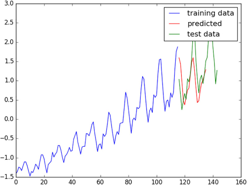
The other graph shows the prediction results when only the training data is given (blue line) and nothing else (see figure 10.7). This procedure has less information available, but it still did a good job matching trends of the data.
Figure 10.7. If the algorithm uses previously predicted results to make further predictions, then the general trend matches well, but not specific bumps.
You can use time-series predictors to reproduce realistic fluctuations in data. Imagine predicting market boom-and-bust cycles based on the tools you’ve learned so far. What are you waiting for? Grab some market data, and learn your own predictive model!
10.5. Application of recurrent neural networks
Recurrent neural networks are meant to be used with sequential data. Because audio signals are a dimension lower than video (linear signal versus two-dimensional pixel array), it’s a lot easier to get started with audio time-series data. Consider how much speech recognition has improved over the years: it’s becoming a tractable problem!
Like the audio histogram analysis you conducted in chapter 5 on clustering audio data, most speech recognition preprocessing involves representing the sound into a chromagram of sorts. Specifically, a common technique is to use a feature called mel-frequency cepstral coefficients (MFCCs). A good introduction is outlined in this blog post: http://mng.bz/411F.
Next, you’ll need a dataset to train your model. A few popular ones include the following:
- LibriSpeech: www.openslr.org/12
- TED-LIUM: www.openslr.org/7
- VoxForge: www.voxforge.org
An in-depth walkthrough of a simple speech-recognition implementation in TensorFlow using these datasets is available online: https://svds.com/tensorflow-rnn-tutorial.
10.6. Summary
- A recurrent neural network (RNN) uses information from the past. That way, it can make predictions using data with high temporal dependencies.
- TensorFlow comes with RNN models out of the box.
- Time-series prediction is a useful application for RNNs because of temporal dependencies in the data.