Chapter 11. Sequence-to-sequence models for chatbots

This chapter covers

• Examining sequence-to-sequence architecture
• Vector embedding of words
• Implementing a chatbot by using real-world data

Talking to customer service over the phone is a burden for both the customer and the company. Service providers pay a good chunk of money to hire these customer service representatives, but what if it’s possible to automate most of this effort? Can we develop software to interface with customers through natural language?

The idea isn’t as farfetched as you might think. Chatbots are getting a lot of hype because of unprecedented developments in natural language processing using deep-learning techniques. Perhaps, given enough training data, a chatbot could learn to navigate the most commonly addressed customer problems through natural conversations. If the chatbot were truly efficient, it could not only save the company money by eliminating the need to hire representatives, but even accelerate the customer’s search for an answer.

In this chapter, you’ll build a chatbot by feeding a neural network thousands of examples of input and output sentences. Your training dataset is a pair of English utterances; for example, if you ask, “How are you?” the chatbot should respond, “Fine, thank you.”

Note

In this chapter, we’re thinking of sequences and sentences as interchangeable concepts. In our implementation, a sentence will be a sequence of letters. Another common approach is to represent a sentence as a sequence of words.

In effect, the algorithm will try to produce an intelligent natural language response to each natural language query. You’ll be implementing a neural network that uses two primary concepts taught in previous chapters: multiclass classification and recurrent neural networks (RNNs).

11.1. Building on classification and RNNs

Remember, classification is a machine-learning approach to predict the category of an input data item. Furthermore, multiclass classification allows for more than two classes. You saw in chapter 4 how to implement such an algorithm in TensorFlow. Specifically, the cost function between the model’s prediction (a sequence of numbers) and the ground truth (a one-hot vector) tries to find the distance between two sequences by using the cross-entropy loss.

Note

A one-hot vector is like an all-zero vector, except one of the dimensions has a value of 1.

In this case, implementing a chatbot, you’ll use a variant of the cross-entropy loss to measure the difference between two sequences: the model’s response (which is a sequence) against the ground truth (which is also a sequence).

You may recall that RNNs are a neural network design for incorporating not only input from the current time step, but also state information from previous inputs. Chapter 10 covered these in great detail, and they’ll be used again in this chapter. RNNs represent input and output as time-series data, which is exactly what you need to represent sequences.

A naïve idea is to use an out-of-the-box RNN to implement a chatbot. Let’s see why this is a bad approach. The input and output of the RNN are natural language sentences, so the inputs (x_t, x_t–1, x_t–2, ...) and outputs (y_t, y_t–1, y_t–2, ...) can be sequences of words. The problem in using an RNN to model conversations is that the RNN produces an output result immediately. If your input is a sequence of words (How, are, you), the first output word will depend on only the first input word. The output sequence item y_t of the RNN couldn’t look ahead to future parts of the input sentence to make a decision; it would be limited by knowledge of only previous input sequences (x_t, x_t–1, x_t–2, ... ). The naïve RNN model tries to come up with a response to the user’s query before they’ve finished asking it, which can lead to incorrect results.

Instead, you’ll end up using two RNNs: one for the input sentence and the other for the output sequence. After the input sequence is finished being processed by the first RNN, it’ll send the hidden state to the second RNN to process the output sentence. You can see the two RNNs labeled Encoder and Decoder in figure 11.1.

Figure 11.1. Here’s a high-level view of your neural network model. The input ayy is passed into the encoder RNN, and the decoder RNN is expected to respond with lmao. These are just toy examples for your chatbot, but you could imagine more-complicated pairs of sentences for the input and output.

We’re bringing concepts of multiclass classification and RNNs from previous chapters into designing a neural network that learns to map an input sequence to an output sequence. The RNNs provide a way of encoding the input sentence, passing a summarized state vector to the decoder, and then decoding it to a response sentence. To measure the cost between the model’s response and the ground truth, we look to the function used in multiclass classification, the cross-entropy loss, for inspiration.

This architecture is called a sequence-to-sequence (seq2seq) neural network architecture. The training data you use will be thousands of pairs of sentences mined from movie scripts. The algorithm will observe these dialogue examples and eventually learn to form responses to arbitrary queries you might ask it.

By the end of the chapter, you’ll have your own chatbot that can respond somewhat intelligently to your queries. It won’t be perfect, because this model always responds the same way for the same input query.

Suppose, for example, that you’re traveling to a foreign country without any ability to speak the language. A clever salesman hands you a book, claiming it’s all you need to respond to sentences in the foreign language. You’re supposed to use it like a dictionary. When someone says a phrase in the foreign language, you can look it up, and the book will have the response written out for you to read aloud: “If someone says Hello, you say Hi.”

Sure, it might be a practical lookup table for small talk, but can a lookup table get you the correct response for arbitrary dialogue? Of course not! Consider looking up the question “Are you hungry?” The answer to that question is stamped in the book and will never change.

The lookup table is missing state information, which is a key component in dialogue. In your seq2seq model, you’ll suffer from a similar issue; but it’s a good start! Believe it or not, as of 2017, hierarchical state representation for intelligent dialogue still isn’t the norm; many chatbots start out with these seq2seq models.

11.2. Seq2seq architecture

The seq2seq model attempts to learn a neural network that predicts an output sequence from an input sequence. Sequences are a little different from traditional vectors, because a sequence implies an ordering of events.

Time is an intuitive way to order events: we usually end up alluding to words related to time, such as temporal, time series, past, and future. For example, we like to say that RNNs propagate information to future time steps. Or, RNNs capture temporal dependencies.

Note

RNNs are covered in detail in chapter 10.

The seq2seq model is implemented using multiple RNNs. A single RNN cell is depicted in figure 11.2; it serves as the building block for the rest of the seq2seq model architecture.

Figure 11.2. The input, output, and states of an RNN. You can ignore the intricacies of exactly how an RNN is implemented. All that matters is the formatting of your input and output.

First, you’ll learn how to stack RNNs on top of each other to improve the model’s complexity. Then you’ll learn how to pipe the hidden state of one RNN to another RNN, so that you can have an “encoder” and “decoder” network. As you’ll begin to see, it’s fairly easy to start using RNNs.

After that, you’ll get an introduction to converting natural language sentences into a sequence of vectors. After all, RNNs understand only numeric data, so you’ll absolutely need this conversion process. Because a sequence is another way of saying “a list of tensors,” you need to make sure you can convert your data accordingly. For example, a sentence is a sequence of words, but words aren’t tensors. The process of converting words to tensors or, more commonly, vectors is called embedding.

Last, you’ll put all these concepts together to implement the seq2seq model on real-world data. The data will come from thousands of conversations from movie scripts.

You can hit the ground running with the following code listing. Open a new Python file, and start copying listing 11.1 to set up constants and placeholders. You’ll define the shape of the placeholder to be [None, seq_size, input_dim], where None means the size is dynamic because the batch size may change, seq_size is the length of the sequence, and input_dim is the dimension of each sequence item.

Listing 11.1. Setting up constants and placeholders

import tensorflow as tf                               1

input_dim = 1                                         2
seq_size = 6                                          3

input_placeholder = tf.placeholder(dtype=tf.float32,
                                   shape=[None, seq_size, input_dim])

• 1 All you need is TensorFlow.
• 2 Dimension of each sequence element
• 3 Maximum length of sequence

To generate an RNN cell like the one in figure 11.2, TensorFlow provides a helpful LSTMCell class. Listing 11.2 shows how to use it and extract the outputs and states from the cell. Just for convenience, the listing defines a helper function called make_cell to set up the LSTM RNN cell. Remember, just defining a cell isn’t enough: you also need to call tf.nn.dynamic_rnn on it to set up the network.

Listing 11.2. Making a simple RNN cell

def make_cell(state_dim):
    return tf.contrib.rnn.LSTMCell(state_dim)                       1

with tf.variable_scope("first_cell") as scope:
    cell = make_cell(state_dim=10)
    outputs, states = tf.nn.dynamic_rnn(cell,                       2
                                        input_placeholder,          3
                                        dtype=tf.float32)

• 1 Check out the tf.contrib.rnn documentation for other types of cells, such as GRU.
• 2 There will be two generated results: outputs and states.
• 3 This is the input sequence to the RNN.

You might remember from previous chapters that you can improve a neural network’s complexity by adding more and more hidden layers. More layers means more parameters, and that likely means the model can represent more functions; it’s more flexible.

You know what? You can stack cells on top of each other. Nothing is stopping you. Doing so makes the model more complex, so perhaps this two-layered RNN model will perform better because it’s more expressive. Figure 11.3 shows two cells stacked together.

Figure 11.3. You can stack RNN cells to form a more complicated architecture.

Warning

The more flexible the model, the more likely that it’ll overfit the training data.

In TensorFlow, you can intuitively implement this two-layered RNN network. First, you create a new variable scope for the second cell. To stack RNNs together, you can pipe the output of the first cell to the input of the second cell. The following listing shows how to do exactly this.

Listing 11.3. Stacking two RNN cells

with tf.variable_scope("second_cell") as scope:                    1
    cell2 = make_cell(state_dim=10)
    outputs2, states2 = tf.nn.dynamic_rnn(cell2,
                                          outputs,                 2
                                          dtype=tf.float32)

• 1 Defining a variable scope helps avoid runtime errors due to variable reuse.
• 2 Input to this cell will be the other cell’s output.

What if you wanted four layers of RNNs? Or 10? For example, figure 11.4 shows four RNN cells stacked atop each other.

Figure 11.4. TensorFlow lets you stack as many RNN cells as you want.

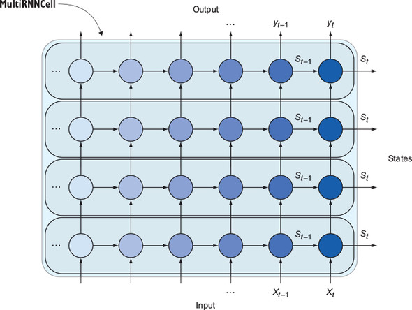
A useful shortcut for stacking cells that the TensorFlow library supplies is called MultiRNNCell. The following listing shows how to use this helper function to build arbitrarily large RNN cells.

Listing 11.4. Using MultiRNNCell to stack multiple cells

def make_multi_cell(state_dim, num_layers):
    cells = [make_cell(state_dim) for _ in range(num_layers)]         1
    return tf.contrib.rnn.MultiRNNCell(cells)

multi_cell = make_multi_cell(state_dim=10, num_layers=4)
outputs4, states4 = tf.nn.dynamic_rnn(multi_cell,
                                      input_placeholder,
                                      dtype=tf.float32)

• 1 The for-loop syntax is the preferred way to construct a list of RNN cells.

So far, you’ve grown RNNs vertically by piping outputs of one cell to the inputs of another. In the seq2seq model, you’ll want one RNN cell to process the input sentence, and another RNN cell to process the output sentence. To communicate between the two cells, you can also connect RNNs horizontally by connecting states from cell to cell, as shown in figure 11.5.

Figure 11.5. You can use the last states of the first cell as the next cell’s initial state. This model can learn mapping from an input sequence to an output sequence. The model is called seq2seq.

You’ve stacked RNN cells vertically and connected them horizontally, vastly increasing the number of parameters in the network! Is this utter blasphemy? Yes. You’ve built a monolithic architecture by composing RNNs every which way. But there’s a method to this madness, because this insane neural network architecture is the backbone of the seq2seq model.

As you can see in figure 11.5, the seq2seq model appears to have two input sequences and two output sequences. But only input 1 will be used for the input sentence, and only output 2 will be used for the output sentence.

You may be wondering what to do with the other two sequences. Strangely enough, the output 1 sequence is entirely unused by the seq2seq model. And, as you’ll see, the input 2 sequence is crafted using some of output 2 data, in a feedback loop.

Your training data for designing a chatbot will be pairs of input and output sentences, so you’ll need to better understand how to embed words into a tensor. The next section covers how to do so in TensorFlow.

11.3. Vector representation of symbols

Words and letters are symbols, and converting symbols to numeric values is easy in TensorFlow. For example, let’s say you have four words in your vocabulary: word₀: the; word₁: fight; word₂: wind; and word₃: like.

Let’s say you want to find the embeddings for the sentence “Fight the wind.” The symbol fight is located at index 1 of the lookup table, the at index 0, and wind at index 2. If you want to find the embedding of the word fight, you have to refer to its index, which is 1, and consult the lookup table at index 1 to identify the embedding value. In our first example, each word is associated with a number, as shown in figure 11.6.

Figure 11.6. A mapping from symbols to scalars

The following listing shows how to define such a mapping between symbols and numeric values using TensorFlow code.

Listing 11.5. Defining a lookup table of scalars

embeddings_0d = tf.constant([17, 22, 35, 51])

Or maybe the words are associated with vectors, as shown in figure 11.7. This is often the preferred method of representing words. You can find a thorough tutorial on vector representation of words in the official TensorFlow docs: http://mng.bz/35M8.

Figure 11.7. A mapping from symbols to vectors

You can implement the mapping between words and vectors in TensorFlow, as shown in the following listing.

Listing 11.6. Defining a lookup table of 4D vectors

embeddings_4d = tf.constant([[1, 0, 0, 0],
                             [0, 1, 0, 0],
                             [0, 0, 1, 0],
                             [0, 0, 0, 1]])

This may sound over the top, but you can represent a symbol by a tensor of any rank you want, not just numbers (rank 0) or vectors (rank 1). In figure 11.8, you’re mapping symbols to tensors of rank 2.

Figure 11.8. A mapping from symbols to tensors

The following listing shows how to implement this mapping of words to tensors in TensorFlow.

Listing 11.7. Defining a lookup table of tensors

embeddings_2x2d = tf.constant([[[1, 0], [0, 0]],
                               [[0, 1], [0, 0]],
                               [[0, 0], [1, 0]],
                               [[0, 0], [0, 1]]])

The embedding_lookup function provided by TensorFlow is an optimized way to access embeddings by indices, as shown in the following listing.

Listing 11.8. Looking up the embeddings

ids = tf.constant([1, 0, 2])                                        1
lookup_0d = sess.run(tf.nn.embedding_lookup(embeddings_0d, ids))
print(lookup_0d)

lookup_4d = sess.run(tf.nn.embedding_lookup(embeddings_4d, ids))
print(lookup_4d)

lookup_2x2d = sess.run(tf.nn.embedding_lookup(embeddings_2x2d, ids))
print(lookup_2x2d)

• 1 Embeddings lookup corresponding to the words fight, the, and wind

In reality, the embedding matrix isn’t something you ever have to hardcode. These listings are for you to understand the ins and outs of the embedding_lookup function in TensorFlow, because you’ll be using it heavily soon. The embedding lookup table will be learned automatically over time by training the neural network. You start by defining a random, normally distributed lookup table. Then, TensorFlow’s optimizer will adjust the matrix values to minimize the cost.

11.4. Putting it all together

The first step in using natural language input in a neural network is to decide on a mapping between symbols and integer indices. Two common ways to represent sentences is by a sequence of letters or a sequence of words. Let’s say, for simplicity, that you’re dealing with sequences of letters, so you’ll need to build a mapping between characters and integer indices.

Note

The official code repository is available at the book’s website (www.manning.com/books/machine-learning-with-tensorflow) and on GitHub (http://mng.bz/EB5A). From there, you can get the code running without needing to copy and paste from the book.

The following listing shows how to build mappings between integers and characters. If you feed this function a list of strings, it’ll produce two dictionaries, representing the mappings.

Listing 11.9. Extracting character vocab

def extract_character_vocab(data):
    special_symbols = ['<PAD>', '<UNK>', '<GO>',  '<EOS>']
    set_symbols = set([character for line in data for character in line])
    all_symbols = special_symbols + list(set_symbols)
    int_to_symbol = {word_i: word
                     for word_i, word in enumerate(all_symbols)}
    symbol_to_int = {word: word_i
                     for word_i, word in int_to_symbol.items()}

    return int_to_symbol, symbol_to_int

input_sentences = ['hello stranger', 'bye bye']                1
output_sentences = ['hiya', 'later alligator']                 2

input_int_to_symbol, input_symbol_to_int =
    extract_character_vocab(input_sentences)

output_int_to_symbol, output_symbol_to_int =
    extract_character_vocab(output_sentences

• 1 List of input sentences for training
• 2 List of corresponding output sentences for training

Next, you’ll define all your hyperparameters and constants in listing 11.10. These are usually values you can tune by hand through trial and error. Typically, greater values for the number of dimensions or layers result in a more complex model, which is rewarding if you have big data, fast processing power, and lots of time.

Listing 11.10. Defining hyperparameters

NUM_EPOCS = 300                                           1
RNN_STATE_DIM = 512                                       2
RNN_NUM_LAYERS = 2                                        3
ENCODER_EMBEDDING_DIM = DECODER_EMBEDDING_DIM = 64        4

BATCH_SIZE = int(32)
LEARNING_RATE = 0.0003

INPUT_NUM_VOCAB = len(input_symbol_to_int)                5
OUTPUT_NUM_VOCAB = len(output_symbol_to_int)              6

• 1 Number of epochs
• 2 RNN’s hidden dimension size
• 3 RNN’s number of stacked cells
• 4 Embedding dimension of sequence elements for the encoder and decoder
• 5 Batch size
• 6 It’s possible to have different vocabularies between the encoder and decoder.

Let’s list all placeholders next. As you can see in listing 11.11, the placeholders nicely organize the input and output sequences necessary to train the network. You’ll have to track both the sequences and their lengths. For the decoder part, you’ll also need to compute the maximum sequence length. The None value in the shape of these placeholders means the tensor may take on an arbitrary size in that dimension. For example, the batch size may vary in each run. But for simplicity, you’ll keep the batch size the same at all times.

Listing 11.11. Listing placeholders

# Encoder placeholders
encoder_input_seq = tf.placeholder(           1
    tf.int32,
    [None, None],                             2
    name='encoder_input_seq'
)

encoder_seq_len = tf.placeholder(             3
    tf.int32,
    (None,),                                  4
    name='encoder_seq_len'
)

# Decoder placeholders
decoder_output_seq = tf.placeholder(          5
    tf.int32,
    [None, None],                             6
    name='decoder_output_seq'
)

decoder_seq_len = tf.placeholder(             7
    tf.int32,
    (None,),                                  8
    name='decoder_seq_len'
)

max_decoder_seq_len = tf.reduce_max(          9
    decoder_seq_len,
    name='max_decoder_seq_len'
)

• 1 Sequence of integers for the encoder’s input
• 2 Shape is batch-size × sequence length
• 3 Lengths of sequences in a batch
• 4 Shape is dynamic because the length of a sequence can change
• 5 Sequence of integers for the decoder’s output
• 6 Shape is batch-size × sequence length
• 7 Lengths of sequences in a batch
• 8 Shape is dynamic because the length of a sequence can change
• 9 Maximum length of a decoder sequence in a batch

Let’s define helper functions to construct RNN cells. These functions, shown in the following listing, should appear familiar to you from the previous section.

Listing 11.12. Helper functions to build RNN cells

def make_cell(state_dim):
    lstm_initializer = tf.random_uniform_initializer(-0.1, 0.1)
    return tf.contrib.rnn.LSTMCell(state_dim, initializer=lstm_initializer)

def make_multi_cell(state_dim, num_layers):
    cells = [make_cell(state_dim) for _ in range(num_layers)]
    return tf.contrib.rnn.MultiRNNCell(cells)

You’ll build the encoder and decoder RNN cells by using the helper functions you’ve just defined. As a reminder, we’ve copied the seq2seq model for you in figure 11.9, to visualize the encoder and decoder RNNs.

Figure 11.9. The seq2seq model learns a transformation between an input sequence to an output sequence by using an encoder RNN and a decoder RNN.

Let’s talk about the encoder cell part first, because in listing 11.13 you’ll build the encoder cell. The produced states of the encoder RNN will be stored in a variable called encoder_state. RNNs also produce an output sequence, but you don’t need access to that in a standard seq2seq model, so you can ignore it or delete it.

It’s also typical to convert letters or words in a vector representation, often called embedding. TensorFlow provides a handy function called embed_sequence that can help you embed the integer representation of symbols. Figure 11.10 shows how the encoder input accepts numeric values from a lookup table. You can see it in action at the beginning of listing 11.13.

Figure 11.10. The RNNs accept only sequences of numeric values as input or output, so you’ll convert your symbols to vectors. In this case, the symbols are words, such as the, fight, wind, and like. Their corresponding vectors are associated in the embedding matrix.

Listing 11.13. Encoder embedding and cell

# Encoder embedding

encoder_input_embedded = tf.contrib.layers.embed_sequence(
    encoder_input_seq,                                             1
    INPUT_NUM_VOCAB,                                               2
    ENCODER_EMBEDDING_DIM                                          3
)


# Encoder output

encoder_multi_cell = make_multi_cell(RNN_STATE_DIM, RNN_NUM_LAYERS)

encoder_output, encoder_state = tf.nn.dynamic_rnn(
    encoder_multi_cell,
    encoder_input_embedded,
    sequence_length=encoder_seq_len,
    dtype=tf.float32
)

del(encoder_output)                                                4

• 1 Input seq of numbers (row indices)
• 2 Rows of embedding matrix
• 3 Columns of embedding matrix
• 4 You don’t need to hold on to that value

The decoder RNN’s output is a sequence of numeric values representing a natural language sentence and a special symbol to represent that the sequence has ended. You’ll label this end-of-sequence symbol as <EOS>. Figure 11.11 illustrates this process. The input sequence to the decoder RNN will look similar to the decoder’s output sequence, except instead of having the <EOS> (end of sequence) special symbol at the end of each sentence, it will have a <GO> special symbol at the front. That way, after the decoder reads its input from left to right, it starts out with no extra information about the answer, making it a robust model.

Figure 11.11. The decoder’s input is prefixed with a special <GO> symbol, whereas the output is suffixed by a special <EOS> symbol.

Listing 11.14 shows how to correctly perform these slicing and concatenating operations. The newly constructed sequence for the decoder’s input will be called decoder_input_seq. You’ll use TensorFlow’s tf.concat operation to glue together matrices. In the listing, you define a go_prefixes matrix, which will be a column vector containing only the <GO> symbol.

Listing 11.14. Preparing input sequences to the decoder

decoder_raw_seq = decoder_output_seq[:, :-1]                            1
go_prefixes = tf.fill([BATCH_SIZE, 1], output_symbol_to_int['<GO>'])    2
decoder_input_seq = tf.concat([go_prefixes, decoder_raw_seq], 1)        3

• 1 Crops the matrix by ignoring the very last column
• 2 Creates a column vector of <GO> symbols
• 3 Concatenates the <GO> vector to the beginning of the cropped matrix

Now let’s construct the decoder cell. As shown in listing 11.15, you’ll first embed the decoder sequence of integers into a sequence of vectors, called decoder_input_ embedded.

The embedded version of the input sequence will be fed to the decoder’s RNN, so go ahead and create the decoder RNN cell. One more thing: you’ll need a layer to map the output of the decoder to a one-hot representation of the vocabulary, which you call output_layer. The process of setting up the decoder starts out to be similar to that with the encoder.

Listing 11.15. Decoder embedding and cell

decoder_embedding = tf.Variable(tf.random_uniform([OUTPUT_NUM_VOCAB,
                                                   DECODER_EMBEDDING_DIM]))
decoder_input_embedded = tf.nn.embedding_lookup(decoder_embedding,
                                                decoder_input_seq)

decoder_multi_cell = make_multi_cell(RNN_STATE_DIM, RNN_NUM_LAYERS)

output_layer_kernel_initializer =
    tf.truncated_normal_initializer(mean=0.0, stddev=0.1)
output_layer = Dense(
    OUTPUT_NUM_VOCAB,
    kernel_initializer = output_layer_kernel_initializer
)

Okay, here’s where things get weird. You have two ways to retrieve the decoder’s output: during training and during inference. The training decoder will be used only during training, whereas the inference decoder will be used for testing on never-before-seen data.

The reason for having two ways to obtain an output sequence is that during training, you have the ground-truth data available, so you can use information about the known output to help speed the learning process. But during inference, you have no ground-truth output labels, so you must resort to making inferences by using only the input sequence.

The following listing implements the training decoder. You’ll feed decoder_input _seq into the decoder’s input, using TrainingHelper. This helper op manages the input to the decoder RNN for you.

Listing 11.16. Decoder output (training)

with tf.variable_scope("decode"):

    training_helper = tf.contrib.seq2seq.TrainingHelper(
        inputs=decoder_input_embedded,
        sequence_length=decoder_seq_len,
        time_major=False
    )

    training_decoder = tf.contrib.seq2seq.BasicDecoder(
        decoder_multi_cell,
        training_helper,
        encoder_state,
        output_layer
    )

    training_decoder_output_seq, _, _ = tf.contrib.seq2seq.dynamic_decode(
        training_decoder,
        impute_finished=True,
        maximum_iterations=max_decoder_seq_len
    )

If you care to obtain output from the seq2seq model on test data, you no longer have access to decoder_input_seq. Why? Well, the decoder input sequence is derived from the decoder output sequence, which is available only with the training dataset.

The following listing implements the decoder output op for the inference case. Here again, you’ll use a helper op to feed the decoder an input sequence.

Listing 11.17. Decoder output (inference)

with tf.variable_scope("decode", reuse=True):
    start_tokens = tf.tile(
        tf.constant([output_symbol_to_int['<GO>']],
                    dtype=tf.int32),
        [BATCH_SIZE],
        name='start_tokens')

    inference_helper = tf.contrib.seq2seq.GreedyEmbeddingHelper(           1
        embedding=decoder_embedding,                                       1
        start_tokens=start_tokens,                                         1
        end_token=output_symbol_to_int['<EOS>']                            1
    )                                                                      1

    inference_decoder = tf.contrib.seq2seq.BasicDecoder(                   2
        decoder_multi_cell,                                                2
        inference_helper,                                                  2
        encoder_state,                                                     2
        output_layer                                                       2
    )                                                                      2

    inference_decoder_output_seq, _, _ = tf.contrib.seq2seq.dynamic_decode(3
        inference_decoder,                                                 3
        impute_finished=True,                                              3
        maximum_iterations=max_decoder_seq_len                             3
    )                                                                      3

• 1 Helper for the inference process
• 2 Basic decoder
• 3 Performs dynamic decoding using the decoder

Compute the cost using TensorFlow’s sequence_loss method. You’ll need access to the inferred decoder output sequence and the ground-truth output sequence. The following listing defines the cost function in code.

Listing 11.18. Cost function

training_logits =                                                          1
    tf.identity(training_decoder_output_seq.rnn_output, name='logits')     1
inference_logits =                                                         1
    tf.identity(inference_decoder_output_seq.sample_id, name='predictions')1

masks = tf.sequence_mask(                                                  2
    decoder_seq_len,                                                       2
    max_decoder_seq_len,                                                   2
    dtype=tf.float32,                                                      2
    name='masks'                                                           2
)                                                                          2

cost = tf.contrib.seq2seq.sequence_loss(                                   3
    training_logits,                                                       3
    decoder_output_seq,                                                    3
    masks                                                                  3
)                                                                          3

• 1 Renames the tensors for your convenience
• 2 Creates the weights for sequence_loss
• 3 Uses TensorFlow’s built-in sequence loss function

Last, let’s call an optimizer to minimize the cost. But you’ll do one trick you might have never seen before. In deep networks like this one, you need to limit extreme gradient change to ensure that the gradient doesn’t change too dramatically, a technique called gradient clipping. Listing 11.19 shows you how to do so.

Listing 11.19. Calling an optimizer

optimizer = tf.train.AdamOptimizer(LEARNING_RATE)

gradients = optimizer.compute_gradients(cost)
capped_gradients = [(tf.clip_by_value(grad, -5., 5.), var)               1
                        for grad, var in gradients if grad is not None]
train_op = optimizer.apply_gradients(capped_gradients)

• 1 Gradient clipping

That concludes the seq2seq model implementation. In general, the model is ready to be trained after you’ve set up the optimizer, as in the previous listing. You can create a session and run train_op with batches of training data to learn the parameters of the model.

Oh, right, you need training data from someplace! How can you obtain thousands of pairs of input and output sentences? Fear not—the next section covers exactly that.

11.5. Gathering dialogue data

The Cornell Movie Dialogues corpus (http://mng.bz/W28O) is a dataset of more than 220,000 conversations from more than 600 movies. You can download the zip file from the official web page.

Warning

Because there’s a huge amount of data, you can expect the training algorithm to take a long time. If your TensorFlow library is configured to use only the CPU, it might take an entire day to train. On a GPU, training this network may take 30 minutes to an hour.

An example of a small snippet of back-and-forth conversation between two people (A and B) is the following:

A: They do not!

B: They do too!

A: Fine.

Because the goal of the chatbot is to produce intelligent output for every possible input utterance, you’ll structure your training data based on contingent pairs of conversation. In the example, the dialogue generates the following pairs of input and output sentences:

• “They do not!” → “They do too!”
• “They do too!” → “Fine.”

For your convenience, we’ve already processed the data and made it available for you online. You can find it at www.manning.com/books/machine-learning-with-tensorflow or http://mng.bz/wWo0. After completing the download, you can run the following listing, which uses the load_sentences helper function from the GitHub repo under the Concept03_seq2seq.ipynb Jupyter Notebook.

Listing 11.20. Training the model

input_sentences = load_sentences('data/words_input.txt')                  1
output_sentences = load_sentences('data/words_output.txt')                2

input_seq = [
    [input_symbol_to_int.get(symbol, input_symbol_to_int['<UNK>'])
        for symbol in line]                                               3
    for line in input_sentences                                           4

]

output_seq = [
    [output_symbol_to_int.get(symbol, output_symbol_to_int['<UNK>'])
        for symbol in line] + [output_symbol_to_int['<EOS>']]             5
    for line in output_sentences                                          6
]

sess = tf.InteractiveSession()
sess.run(tf.global_variables_initializer())
saver = tf.train.Saver()                                                  7

for epoch in range(NUM_EPOCS + 1):                                        7

    for batch_idx in range(len(input_sentences) // BATCH_SIZE):           9

        input_data, output_data = get_batches(input_sentences,            10
                                              output_sentences,
                                              batch_idx)


        input_batch, input_lenghts = input_data[batch_idx]
        output_batch, output_lengths = output_data[batch_idx]

        _, cost_val = sess.run(                                           11
            [train_op, cost],
            feed_dict={
                encoder_input_seq: input_batch,
                encoder_seq_len: input_lengths,
                decoder_output_seq: output_batch,
                decoder_seq_len: output_lengths
            }
        )

saver.save(sess, 'model.ckpt')
sess.close()

• 1 Loads the input sentences as a list of strings
• 2 Loads the corresponding output sentences the same way
• 3 Loops through the letters
• 4 Loops through the lines of text
• 5 Appends the EOS symbol to the end of the output data
• 6 Loops through the lines
• 7 It’s a good idea to save the learned parameters.
• 8 Loops through the epochs
• 9 Loops by the number of batches
• 10 Gets input and output pairs for the current batch
• 11 Runs the optimizer on the current batch

Because you saved the model parameters to a file, you can easily load it onto another program and query the network for responses to new input. Run the inference_logits op to obtain the chatbot response.

11.6. Summary

In this chapter, you built a real-world example of a seq2seq network, putting to work all the TensorFlow knowledge you learned in the previous chapters:

• You built a seq2seq neural network by putting to work all the TensorFlow knowledge you’ve acquired from the book so far.
• You learned how to embed natural language in TensorFlow.
• You used RNNs as a building block for a more interesting model.
• After training the model on examples of dialogue from movie scripts, you were able to treat the algorithm like a chatbot, inferring natural language responses from natural language input.