Chapter 12. Utility landscape

This chapter covers

• Implementing a neural network for ranking
• Image embedding using VGG16
• Visualizing utility

A household vacuuming robot, like the Roomba, needs sensors to “see” the world. The ability to process sensory input enables robots to adjust their model of the world around them. In the case of the vacuum cleaner robot, the furniture in the room may change day to day, so the robot must be able to adapt to chaotic environments.

Let’s say you own a futuristic housemaid robot, which comes with a few basic skills but also with the ability to learn new skills from human demonstrations. For example, maybe you’d like to teach it how to fold clothes.

Teaching a robot how to accomplish a new task is a tricky problem. Some immediate questions come to mind:

• Should the robot simply mimic a human’s sequence of actions? Such a process is referred to as imitation learning.
• How do a robot’s arms and joints match up to human poses? This dilemma is often referred to as the correspondence problem.

In this chapter, you’re going to model a task from human demonstrations while avoiding both imitation learning and the correspondence problem. Lucky you! You’ll achieve this by studying a way to rank states of the world with a utility function, which is a function that takes a state and returns a real value representing its desirability. Not only will you steer clear of imitation as a measure of success, but you’ll also bypass the complications of mapping a robot’s set of actions to that of a human (the correspondence problem).

In the following section, you’ll learn how to implement a utility function over the states of the world obtained through videos of human demonstrations of a task. The learned utility function is a model of preferences.

You’ll explore the task of teaching a robot how to fold articles of clothing. A wrinkled article of clothing is almost certainly in a configuration that has never before been seen. As shown in figure 12.1, the utility framework has no limitations on the size of the state space. The preference model is trained specifically on videos of people folding T-shirts in various ways.

Figure 12.1. Wrinkled clothes in a less favorable state than well-folded clothes. This diagram shows how you might score each state of a piece of cloth; higher scores represent a more favorable state.

The utility function generalizes across states (wrinkled T-shirt in novel configuration versus folded T-shirt in familiar configuration) and reuses knowledge across clothes (T-shirt folding versus pants folding).

We can further illustrate the practical applications of a good utility function with the following argument: in real-world situations, not all visual observations are optimized toward learning a task. A teacher demonstrating a skill may perform irrelevant, incomplete, or even incorrect actions, yet humans are capable of ignoring the mistakes.

When a robot watches human demonstrations, you want it to understand the causal relationships that go into achieving a task. Your work enables the learning phase to be interactive, where the robot is actively skeptic of human behavior, to refine the training data.

To accomplish this, you first learn a utility function from a small number of videos to rank the preferences of various states. Then, when the robot is shown a new instance of a skill through human demonstration, it consults the utility function to verify that the expected utility increases over time. Lastly, the robot interrupts the human demonstration to ask whether the action was essential for learning the skill.

12.1. Preference model

We assume human preferences are derived from a utilitarian perspective, meaning a number determines the rank of items. For example, suppose you surveyed people to rank the fanciness of various foods (such as steak, hotdog, shrimp cocktail, and burger).

Figure 12.2 shows a couple of possible rankings between pairs of food. As you might expect, steak is ranked higher than hotdog, and shrimp cocktail higher than burger on the fanciness scale.

Figure 12.2. This is a possible set of pairwise rankings between objects. Specifically, you have four food items, and you want to rank them by fanciness, so you employ two pairwise ranking decisions: steak is a fancier meal than a hotdog, and shrimp cocktail is a fancier meal than a burger.

Fortunately for the individuals being surveyed, not every pair of items needs to be ranked. For example, it might not be so obvious which is fancier between hotdog and burger, or between steak and shrimp cocktail. There’s a lot of room for disagreement.

If a state s₁ has a higher utility than another state s₂, then the corresponding ranking is denoted s₁ > s₂, implying the utility of s₁ is greater than the utility of s₂. Each video demonstration contains a sequence of n states s₀, s₁, .., s_n, which offers n(n – 1)/2 possible ordered pairs ranking constraints. Let’s implement our own neural network capable of ranking. Open a new source file, and use the following listing to import the relevant libraries. You’re about to create a neural network to learn a utility function based on pairs of preferences.

Listing 12.1. Importing relevant libraries

import tensorflow as tf
import numpy as np
import random

%matplotlib inline
import matplotlib.pyplot as plt

To learn a neural network for ranking states based on a utility score, you’ll need training data. Let’s create dummy data to begin with. You’ll replace it with something more realistic later. Reproduce the two-dimensional data in figure 12.3 by using listing 12.2.

Listing 12.2. Generating dummy training data

n_features = 2                                                1

def get_data():
    data_a = np.random.rand(10, n_features) + 1               2
    data_b = np.random.rand(10, n_features)                   3

    plt.scatter(data_a[:, 0], data_a[:, 1], c='r', marker='x')
    plt.scatter(data_b[:, 0], data_b[:, 1], c='g', marker='o')
    plt.show()

    return data_a, data_b

data_a, data_b = get_data()

• 1 You’ll generate two-dimensional data so that you can easily visualize it.
• 2 The set of points that should yield higher utility
• 3 The set of points that are less preferred

Figure 12.3. Example data that you’ll work with. The circles represent morefavorable states, whereas the crosses represent less-favorable states. You have an equal number of circles and crosses because the data comes in pairs; each pair is a ranking, as in figure 12.2.

Next, you need to define hyperparameters. In this model, let’s stay simple by keeping the architecture shallow. You’ll create a network with just one hidden layer. The corresponding hyperparameter that dictates the hidden layer’s number of neurons is the following:

n_hidden = 10

The ranking neural network will receive pairwise input, so you’ll need to have two separate placeholders, one for each part of the pair. Moreover, you’ll create a placeholder to hold the dropout parameter value. Continue by adding the following listing to your script.

Listing 12.3. Placeholders

with tf.name_scope("input"):
    x1 = tf.placeholder(tf.float32, [None, n_features], name="x1")         1
    x2 = tf.placeholder(tf.float32, [None, n_features], name="x2")         2
    dropout_keep_prob = tf.placeholder(tf.float32, name='dropout_prob')

• 1 Input placeholder for preferred points
• 2 Input placeholder for non-preferred points

The ranking neural network will contain only one hidden layer. In the following listing, you define the weights and biases, and then reuse these weights and biases on each of the two input placeholders.

Listing 12.4. Hidden layer

with tf.name_scope("hidden_layer"):
    with tf.name_scope("weights"):
        w1 = tf.Variable(tf.random_normal([n_features, n_hidden]), name="w1")
        tf.summary.histogram("w1", w1)
        b1 = tf.Variable(tf.random_normal([n_hidden]), name="b1")
        tf.summary.histogram("b1", b1)

    with tf.name_scope("output"):
        h1 = tf.nn.dropout(tf.nn.relu(tf.matmul(x1,w1) + b1),
     keep_prob=dropout_keep_prob)
        tf.summary.histogram("h1", h1)
        h2 = tf.nn.dropout(tf.nn.relu(tf.matmul(x2, w1) + b1),
     keep_prob=dropout_keep_prob)
        tf.summary.histogram("h2", h2)

The goal of the neural network is to calculate a score for the two inputs provided. In the following listing, you define the weights, biases, and fully connected architecture of the output layer of the network. You’ll be left with two output vectors, s1 and s2, representing the scores for the pairwise input.

Listing 12.5. Output layer

with tf.name_scope("output_layer"):
    with tf.name_scope("weights"):
        w2 = tf.Variable(tf.random_normal([n_hidden, 1]), name="w2")
        tf.summary.histogram("w2", w2)
        b2 = tf.Variable(tf.random_normal([1]), name="b2")
        tf.summary.histogram("b2", b2)

    with tf.name_scope("output"):
        s1 = tf.matmul(h1, w2) + b2            1
        s2 = tf.matmul(h2, w2) + b2            2

• 1 Utility score of input x1
• 2 Utility score of input x2

You’ll assume that when training the neural network, x1 should contain the less-favorable items. That means s1 should be scored lower than s2, meaning the difference between s1 and s2 should be negative. As the following listing shows, the loss function tries to guarantee a negative difference by using the softmax cross-entropy loss. You’ll define a train_op to minimize the loss function.

Listing 12.6. Loss and optimizer

with tf.name_scope("loss"):
    s12 = s1 - s2
    s12_flat = tf.reshape(s12, [-1])

    cross_entropy = tf.nn.softmax_cross_entropy_with_logits(
                        labels=tf.zeros_like(s12_flat),
                        logits=s12_flat + 1)

    loss = tf.reduce_mean(cross_entropy)
    tf.summary.scalar("loss", loss)

with tf.name_scope("train_op"):
    train_op = tf.train.AdamOptimizer(0.001).minimize(loss)

Now, follow listing 12.7 to set up a TensorFlow session. This involves initializing all variables and preparing TensorBoard debugging by using a summary writer.

Note

You used a summary writer before, at the end of chapter 2, when you were first introduced to TensorBoard.

Listing 12.7. Preparing a session

sess = tf.InteractiveSession()
summary_op = tf.summary.merge_all()
writer = tf.summary.FileWriter("tb_files", sess.graph)
init = tf.global_variables_initializer()
sess.run(init)

You’re ready to train the network! Run train_op on the dummy data you generated to learn the parameters of the model.

Listing 12.8. Training the network

for epoch in range(0, 10000):
    loss_val, _ = sess.run([loss, train_op], feed_dict={x1:data_a, x2:data_b,
     dropout_keep_prob:0.5})                                               1
    if epoch % 100 == 0 :
        summary_result = sess.run(summary_op,
                                  feed_dict={x1:data_a,                    2
                                             x2:data_b,                    3
                                             dropout_keep_prob:1})         4
        writer.add_summary(summary_result, epoch)

• 1 Training dropout keep_prob is 0.5.
• 2 Preferred points
• 3 Non-preferred points
• 4 Testing dropout keep_prob should always be 1.

Finally, let’s visualize the learned score function. As shown in the following listing, append two-dimensional points to a list.

Listing 12.9. Preparing test data

grid_size = 10
data_test = []
for y in np.linspace(0., 1., num=grid_size):              1
    for x in np.linspace(0., 1., num=grid_size):          2
        data_test.append([x, y])

• 1 Loops through the rows
• 2 Loops through the columns

You’ll run the s1 op on the test data to obtain utility values of each state, and visualize it as shown in figure 12.4. Use the following listing to generate the visualization.

Listing 12.10. Visualize results

def visualize_results(data_test):
    plt.figure()
    scores_test = sess.run(s1, feed_dict={x1:data_test, dropout_keep_prob:1})1
    scores_img = np.reshape(scores_test, [grid_size, grid_size])             2
    plt.imshow(scores_img, origin='lower')
    plt.colorbar()

visualize_results(data_test)

• 1 Computes the utility of all the points
• 2 Reshapes the utilities to a matrix so you can visualize an image using Matplotlib

Figure 12.4. The landscape of scores learned by the ranking neural network

12.2. Image embedding

In chapter 11, you summoned the hubris to feed a neural network some natural language sentences. You did so by converting words or letters in a sentence into numeric forms, such as vectors. For example, each symbol (whether it’s a word or letter) was embedded into a vector by using a lookup table.

Fortunately, images are already in a numeric form. They’re represented as a matrix of pixels. If the image is grayscale, perhaps the pixels take on scalar values indicating luminosity. For colored images, each pixel represents color intensities (usually three: red, green, and blue). Either way, an image can easily be represented by numeric data structures, such as a tensor, in TensorFlow.

Feeding a neural network a large image, say of size 1280 × 720 (almost 1 million pixels), increases the number of parameters and, consequently, escalates the risk of overfitting the model. The pixels in an image are highly redundant, so you can try to somehow capture the essence of an image in a more succinct representation. Figure 12.5 shows the clusters formed in a two-dimensional embedding of images of clothes being folded.

Figure 12.5. Images can be embedded into much lower dimensions, such as 2D as shown here. Notice that points representing similar states of a shirt occur in nearby clusters. Embedding images allows you to use the ranking neural network to learn a preference between the states of a piece of cloth.

You saw in chapter 7 how to use autoencoders to reduce the dimensionality of images. Another common way to accomplish low-dimensional embedding of images is by using the penultimate layer of a deep convolutional neural network image classifier. Let’s explore the latter in more detail.

Because designing, implementing, and learning a deep image classifier isn’t the primary focus of this chapter (see chapter 9 for CNNs), you’ll instead use an off-the-shelf pretrained model. A common go-to image classifier that many computer vision research papers cite is called VGG16.

Many online implementations of VGG16 exist for TensorFlow. We recommend using the one by Davi Frossard (www.cs.toronto.edu/~frossard/post/vgg16/). You can download the vgg16.py TensorFlow code and the vgg16_weights.npz pretrained model parameters from his website or, alternatively, from the book’s website (www.manning.com/books/machine-learning-with-tensorflow) or GitHub repo (https://github.com/BinRoot/TensorFlow-Book).

Figure 12.6 is a depiction of the VGG16 neural network from Frossard’s page. As you see, it’s a deep neural network, with many convolutional layers. The last few are the usual fully connected layers, and, finally, the output layer is a 1,000-dimensional vector indicating the multiclass classification probabilities.

Figure 12.6. The VGG16 architecture is a deep convolutional neural network used for classifying images. This particular diagram is from www.cs.toronto.edu/~frossard/post/vgg16/.

Learning how to navigate other people’s code is an indispensable skill. First, make sure you have vgg16.py and vgg16_weights.npz downloaded, and test that you’re able to run the code by using python vgg16.py my_image.png.

Note

You might need to install SciPy and Pillow to get the VGG16 demo code to run without issues. You can download both via pip.

Let’s start by adding TensorBoard integration to visualize what’s going on in this code. In the main function, after creating a session variable sess, insert the following line of code:

my_writer = tf.summary.FileWriter('tb_files', sess.graph

Now, running the classifier once again (python vgg16.py my_image.png) will generate a directory called tb_files, to be used by TensorBoard. You can run TensorBoard to visualize the computation graph of the neural network. The following command runs TensorBoard:

$ tensorboard --logdir=tb_files

Open TensorBoard in your browser, and navigate to the Graphs tab to see the computation graph, as shown in figure 12.7. Notice that with a quick glance, you can immediately get an idea of the types of layers involved in the network: the last three layers are fully connected dense layers, labeled fc1, fc2, and fc3.

Figure 12.7. A small segment of the computation graph shown in TensorBoard for the VGG16 neural network. The topmost node is the softmax operator used for classification. The three fully connected layers are labeled fc1, fc2, and fc3.

12.3. Ranking images

You’ll use the VGG16 code in the previous section to obtain a vector representation of an image. That way, you can rank two images efficiently in the ranking neural network designed in section 12.1.

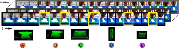
Consider videos of shirt-folding, as shown in figure 12.8. You’ll process videos frame by frame to rank the states of the images. That way, in a novel situation, the algorithm can understand whether the goal of cloth-folding has been reached.

Figure 12.8. Videos of folding a shirt reveal how the cloth changes form through time. You can extract the first state and the last state of the shirt as your training data to learn a utility function to rank states. Final states of shirt in each video should be ranked with a higher utility than those shirts near the beginning of the video.

First, download the cloth-folding dataset from http://mng.bz/eZsc. Extract the zip. Keep note of where you extract it; you’ll call that location DATASET_DIR in the code listings.

Open a new source file, and begin by importing the relevant libraries in Python.

Listing 12.11. Importing libraries

import tensorflow as tf
import numpy as np
from vgg16 import vgg16
import glob, os
from scipy.misc import imread, imresize

For each video, you’ll remember the first and last images. That way, you can train the ranking algorithm by assuming the last image is of a higher preference than the first image. In other words, the last state of cloth-folding brings you to a higher-valued state than the first state of cloth-folding. The following listing shows an example of how to load the data into memory.

Listing 12.12. Preparing the training data

DATASET_DIR = os.path.join(os.path.expanduser('~'), 'res',
     'cloth_folding_rgb_vids')                                          1
NUM_VIDS = 45                                                           2

def get_img_pair(video_id):                                             3
    img_files = sorted(glob.glob(os.path.join(DATASET_DIR, video_id,
     '*.png')))
    start_img = img_files[0]
    end_img = img_files[-1]
    pair = []
    for image_file in [start_img, end_img]:
        img_original = imread(image_file)
        img_resized = imresize(img_original, (224, 224))
        pair.append(img_resized)
    return tuple(pair)

start_imgs = []
end_imgs= []
for vid_id in range(1, NUM_VIDS + 1):
    start_img, end_img = get_img_pair(str(vid_id))
    start_imgs.append(start_img)
    end_imgs.append(end_img)
print('Images of starting state {}'.format(np.shape(start_imgs)))
print('Images of ending state {}'.format(np.shape(end_imgs)))

• 1 Directory of downloaded files
• 2 Number of videos to load
• 3 Gets the starting and ending image of a video

Running listing 12.12 results in the following output:

Images of starting state (45, 224, 224, 3)
Images of ending state (45, 224, 224, 3)

Use the following listing to create an input placeholder for the image that you’ll be embedding.

Listing 12.13. Placeholder

imgs_plc = tf.placeholder(tf.float32, [None, 224, 224, 3])

Copy over the ranking neural network code from listings 12.3–12.7; you’ll reuse it to rank images. Then prepare the session in the following listing.

Listing 12.14. Preparing the session

sess = tf.InteractiveSession()
sess.run(tf.global_variables_initializer())

Next, you’ll initialize the VGG16 model by calling the constructor. Doing so, as shown next, loads all the model parameters from disk to memory.

Listing 12.15. Loading the VGG16 model

print('Loading model...')
vgg = vgg16(imgs_plc, 'vgg16_weights.npz', sess)
print('Done loading!')

Next, let’s prepare training and testing data for the ranking neural network. As shown in listing 12.16, you’ll feed the VGG16 model your images, and then you’ll access a layer near the output (in this case, fc1) to obtain the image embedding.

In the end, you’ll have a 4,096-dimensional embedding of your images. Because there are a total of 45 videos, you’ll split some for training and some for testing:

• Train
  • Start-frame size: (33, 4096)
  • End-frame size: (33, 4096)
• Test
  • Start-frame size: (12, 4096)
  • End-frame size: (12, 4096)

Listing 12.16. Preparing data for ranking

start_imgs_embedded = sess.run(vgg.fc1, feed_dict={vgg.imgs: start_imgs})
end_imgs_embedded = sess.run(vgg.fc1, feed_dict={vgg.imgs: end_imgs})

idxs = np.random.choice(NUM_VIDS, NUM_VIDS, replace=False)
train_idxs = idxs[0:int(NUM_VIDS * 0.75)]
test_idxs = idxs[int(NUM_VIDS * 0.75):]

train_start_imgs = start_imgs_embedded[train_idxs]
train_end_imgs = end_imgs_embedded[train_idxs]
test_start_imgs = start_imgs_embedded[test_idxs]
test_end_imgs = end_imgs_embedded[test_idxs]

print('Train start imgs {}'.format(np.shape(train_start_imgs)))
print('Train end imgs {}'.format(np.shape(train_end_imgs)))
print('Test start imgs {}'.format(np.shape(test_start_imgs)))
print('Test end imgs {}'.format(np.shape(test_end_imgs)))

With your training data ready for ranking, let’s run train_op an epoch number of times. After training the network, run the model on the test data to evaluate your results.

Listing 12.17. Training the ranking network

train_y1 = np.expand_dims(np.zeros(np.shape(train_start_imgs)[0]), axis=1)
train_y2 = np.expand_dims(np.ones(np.shape(train_end_imgs)[0]), axis=1)
for epoch in range(100):
    for i in range(np.shape(train_start_imgs)[0]):
        _, cost_val = sess.run([train_op, loss],
                               feed_dict={x1: train_start_imgs[i:i+1,:],
                                          x2: train_end_imgs[i:i+1,:],
                                          dropout_keep_prob: 0.5})
    print('{}. {}'.format(epoch, cost_val))
    s1_val, s2_val = sess.run([s1, s2], feed_dict={x1: test_start_imgs,
                                                   x2: test_end_imgs,
                                                   dropout_keep_prob: 1})
    print('Accuracy: {}%'.format(100 * np.mean(s1_val < s2_val)))

Notice that the accuracy approaches 100% over time. Your ranking model learns that the images that occur at the end of the video are more favorable than the images that occur near the beginning.

Just out of curiosity, let’s see the utility over time of a single video, frame by frame, as shown in figure 12.9. The code to reproduce figure 12.9 requires loading all the images in a video, as outlined in listing 12.18.

Figure 12.9. The utility increases over time, indicating the goal is being accomplished. The utility of the cloth near the beginning of the video is near 0, but it dramatically increases to 120,000 units by the end.

Listing 12.18. Preparing image sequences from video

def get_img_seq(video_id):
    img_files = sorted(glob.glob(os.path.join(DATASET_DIR, video_id, '*.png')))
    imgs = []
    for image_file in img_files:
        img_original = imread(image_file)
        img_resized = imresize(img_original, (224, 224))
        imgs.append(img_resized)
    return imgs

imgs = get_img_seq('1')

You can use your VGG16 model to embed the images, and then run the ranking network to compute the scores, as shown in the following listing.

Listing 12.19. Computing the utility of images

imgs_embedded = sess.run(vgg.fc1, feed_dict={vgg.imgs: imgs})
scores = sess.run([s1], feed_dict={x1: imgs_embedded,
                                   dropout_keep_prob: 1})

Visualize your results to reproduce figure 12.9.

Listing 12.20. Visualizing utility scores

from matplotlib import pyplot as plt
plt.figure()
plt.title('Utility of cloth-folding over time')
plt.xlabel('time (video frame #)')
plt.ylabel('Utility')
plt.plot(scores[-1])

12.4. Summary

• You can rank states by representing objects as vectors and learning a utility function over such vectors.
• Because images contain redundant data, you used the VGG16 neural network to reduce the dimensionality of your data so that you can use the ranking network with real-world images.
• You learned how to visualize the utility of images over time in a video, to verify that the video demonstration increases the utility of the cloth.

You’ve finished your TensorFlow journey! The 12 chapters of this book approached ML from different angles; but together, they taught you the concepts required to master these skills:

• Formulating an arbitrary real-world problem into a machine-learning framework
• Understanding the basics of many machine-learning problems
• Using TensorFlow to solve these machine-learning problems
• Visualizing a machine-learning algorithm, and speaking the lingo

12.5. What’s next?

Because the concepts taught in this book are timeless, the code listings should be, too. To ensure the most up-to-date library calls and syntax, we actively manage a GitHub repository at https://github.com/BinRoot/TensorFlow-Book. Please feel free to join the community there and file bugs or send us pull requests.

Tip

TensorFlow is in a state of rapid development, so more functionality will become available all the time!

If you’re thirsty for more TensorFlow tutorials, we know exactly what might interest you:

• Reinforcement learning (RL)—An in-depth series of blog posts by Arthur Juliani on using RL in TensorFlow: http://mng.bz/C17q.
• Natural language processing (NLP)—An essential TensorFlow guide to modern neural network architectures in NLP, by Thushan Ganegedara: http://mng.bz/2Kh7.
• Generative adversarial networks (GAN)—An introductory study of generative versus discriminative models in machine learning (using TensorFlow), by John Glover at AYLIEN: http://mng.bz/o2gc.
• Web tool—Tinker with a simple neural network to visualize the flow of data: http://playground.tensorflow.org.
• Video lectures—Basic introduction and hands-on demos using TensorFlow, on the Google Cloud Big Data and Machine Learning Blog: http://mng.bz/vb7U.
• Open source projects—Follow along with the most recently updated TensorFlow projects on GitHub: http://mng.bz/wVZ4