
Chapter 5
Brief Overview of Probability
OBJECTIVE OF THE CHAPTER
The principles of machine learning are largely dependent on effectively handling the uncertainty in data and predicting the outcome based on data in hand. All the learning processes we will be discussing in later chapters of this book expects the readers to understand the foundational rules of probability, the concept of random and continuous variables, distribution, and sampling principles and few basic principles such as central limit theorem, hypothesis testing, and Monte Carlo approximations. As these rules, theorems, and principles form the basis of learning principles, we will be discussing those in this chapter with examples and illustrations.
5.1 INTRODUCTION
As we discussed in previous chapters, machine learning provides us a set of methods that can automatically detect patterns in data, and then can be used to uncover patterns to predict future data, or to perform other kinds of decision making under uncertainty. The best way to perform such activities on top of huge data set known as big data is to use the tools of probability theory because probability theory can be applied to any situation involving uncertainty. In machine learning there may be uncertainties in different forms like arriving at the best prediction of future given the past data, arriving at the best model based on certain data, arriving at the confidence level while predicting the future outcome based on past data, etc. The probabilistic approach used in machine learning is closely related to the field of statistics, but the emphasis is in a different direction as we see in this chapter. In this chapter we will discuss the tools, equations, and models of probability that are useful for machine learning domain.
5.2 IMPORTANCE OF STATISTICAL TOOLS IN MACHINE LEARNING
In machine learning, we train the system by using a limited data set called ‘training data’ and based on the confidence level of the training data we expect the machine learning algorithm to depict the behaviour of the larger set of actual data. If we have observation on a subset of events, called ‘sample’, then there will be some uncertainty in attributing the sample results to the whole set or population. So, the question was how a limited knowledge of a sample set can be used to predict the behaviour of a real set with some confidence. It was realized by mathematicians that even if some knowledge is based on a sample, if we know the amount of uncertainty related to it, then it can be used in an optimum way without causing loss of knowledge. Refer Figure 5.1
FIG. 5.1 Knowledge and uncertainty
Probability theory provides a mathematical foundation for quantifying this uncertainty of the knowledge. As the knowledge about the training data comes in the form of interdependent feature sets, the conditional probability theories (especially the Bayes theorem), discussed later in this chapter form the basis for deriving required confidence level of the training data.
Different distribution principles discussed in this chapter create the view of how the data set that we will be dealing with in machine learning can behave, in terms of their feature distributions. It is important to understand the mathematical function behind each of these distributions so that we can understand how the data is spread out from its average value – denoted by the mean and the variance. While choosing the samples from these distribution sets we should be able to calculate to what extent the sample is representing the actual behaviour of the full data set. These along with the test of hypothesis principles build the basis for finding out the uncertainty in the training data set to represent the actual data set which is the fundamental principle of machine learning.
5.3 CONCEPT OF PROBABILITY – FREQUENTIST AND BAYESIAN INTERPRETATION
The concept of probability is not new. In our day to day life, we use the concept of probability in many places. For example, when we talk about probabilities of getting the heads and the tails when a coin is flipped are equal, we actually intend to say that if a coin is flipped many times, the coin will land heads a same number of times as it lands tails. This is the frequentist interpretation of probability. This interpretation represents the long run frequencies of events. Another important interpretation of probability tries to quantify the uncertainty of some event and thus focuses on information rather than repeated trials. This is called the Bayesian interpretation of probability. Taking the same example of coin flipping is interpreted as – the coin is equally likely to land heads or tails when we flip the coin next.
The reason the Bayesian interpretation can be used to model the uncertainty of events is that it does not expect the long run frequencies of the events to happen. For example, if we have to compute the probability of Brazil winning 2018 football world cup final, that event can happen only once and can’t be repeated over and over again to calculate its probability. But still, we should be able to quantify the uncertainty about the event and which is only possible if we interpret probability the Bayesian way. To give some more machine learning oriented examples, we are starting a new software implementation project for a large customer and want to compute the probability of this project getting into customer escalation based on data from similar projects in the past, or we want to compute the probability of a tumor to be malignant or not based on the probability distribution of such cases among the patients of similar profile. In all these cases it is not possible to do a repeated trial of the event and the Bayesian concept is valid for computing the uncertainty. So, in this book, we will focus on the Bayesian interpretation to develop our machine learning models. The basic formulae of probability remain the same anyway irrespective of whatever interpretation we adopt.
5.3.1 A brief review of probability theory
We will briefly touch upon the basic probability theory in this section just as a refresher so that we can move to the building blocks of machine learning way of use of probability. As discussed in previous chapters, the basic concept of machine learning is that we want to have a limited set of ‘Training’ data that we use as a representative of a large set of Actual data and through probability distribution we try to find out how an event which is matching with the training data can represent the outcome with some confidence.
5.3.1.1 Foundation rules
We will review the basic rules of probability in this section.
Let us introduce few notations that will be used throughout this book.
p(A) denotes the probability that the event A is true. For example, A might be the logical statement ‘Brazil is going to win the next football world cup final’. The expression 0 ≤ p(A) ≤ 1 denotes that the probability of this event happening lies between 0 and 1, where p(A) = 0 means the event will definitely not happen, and p(A) = 1 means the event will definitely happen. The notation p(A̅) denotes the probability of the event not A; this is defined as p(A̅) = 1 − p(A). It is also common practice to write A = 1 to mean the event A is true, and A = 0 to mean the event A is false. So, this is a binary event where the event is either true or false but can’t be something indefinite.
The probability of selecting an event A, from a sample size of X is defined as
p(A) = ![]() , where n is the number of times the instance of event A is present in the sample of size X.
, where n is the number of times the instance of event A is present in the sample of size X.
5.3.1.2 Probability of a union of two events
Two events A and B are called mutually exclusive if they can’t happen together. For example, England winning the Football World Cup 2018 and Brazil winning the Football World Cup 2018 are two mutually exclusive events and can’t happen together. For any two events, A and B, we define the probability of A or B as
5.3.1.3 Joint probabilities
The probability of the joint event A and B is defined as the product rule:
where p(A|B) is defined as the conditional probability of event A happening if event B happens. Based on this joint distribution on two events p(A, B),we can define the marginal distribution as follows:
summing up the all probable states of B gives the total probability formulae, which is also called sum rule or the rule of total probability.
Same way, p(B) can be defined as
This formula can be extended for the countably infinite number of events in the set and chain rule of probability can be derived if the product rule is applied multiple times as
5.3.1.4 Conditional probability
We define the conditional probability of event A, given that event B is true, as follows:
where, p(A, B) is the joint probability of A and B and can also be denoted as p(A ∩ B)
Illustration. In a toy-making shop, the automated machine produces few defective pieces. It is observed that in a lot of 1,000 toy parts, 25 are defective. If two random samples are selected for testing without replacement (meaning that the first sample is not put back to the lot and thus the second sample is selected from the lot size of 999) from the lot, calculate the probability that both the samples are defective.
Solution: Let A denote the probability of first part being defective and B denote the second part being defective. Here, we have to employ the conditional probability of the second part being found defective when the first part is already found defective.
By law of probability, p(A) = ![]()
As we are selecting the second sample without replacing the first sample into the lot and the first one is already found defective, there are now 24 defective pieces out of 999 pieces left in the lot.
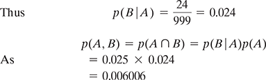
which is the probability of both the parts being found defective.
5.3.1.5 Bayes rule
The Bayes rule, also known as Bayes Theorem, can be derived by combining the definition of conditional probability with the product and sum rules, as below:
Illustration: Flagging an email as spam based on the sender name of the email
Let’s take an example to identify the probability of an email to be really spam based on the name of the sender. We often receive email from mail id containing junk characters or words such as bulk, mass etc. which turn out to be a spam mail. So, we want our machine learning agent to flag the spam emails for us so that we can easily delete them.
Let’s also assume that we have knowledge about the reliability of the assumption that emails with sender names ‘mass’ and ‘bulk’ are spam email is 80% meaning that if some email has sender name with ‘mass’ or ‘bulk’ then the email will be spam with probability 0.8. The probability of false alarm is 10% meaning that the agent will show the positive result as spam even if the email is not a spam with a probability 0.1. Also, we have a prior knowledge that only 0.4% of the total emails received are spam.
Solution:
Let x be the event of the flag being set as spam because the sender name has the words ‘mass’ or ‘bulk’ and y be the event of some mail really being spam.
So, p(x = 1|y = 1) = 0.8, which is the probability of the flag being positive if the email is spam.
Many times this probability is wrongly interpreted as the probability of an email being spam if the flag is positive. But that is not true, because we will then ignore the prior knowledge that only 0.4% of the emails are actually spam and also there can be a false alarm in 10% of the cases.
So, p(y = 1) = 0.004 and p(y = 0) = 1 − p(y = 1) = 0.996
Combining these terms using the Bayes rule, we can compute the correct answer as follows:
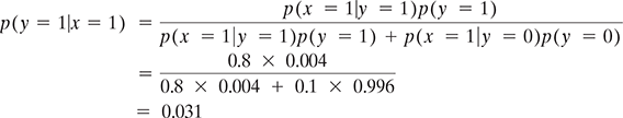
This means that if we combine our prior knowledge with the actual test results then there is only about a 3% chance of emails actually being spam if the sender name contains the terms ‘bulk’ or ‘mass’. This is significantly lower than the earlier assumption of 80% chance and thus calls for additional checks before someone starts deleting such emails based on only this flag.
Details of the practice application of Bayes theorem in machine learning is discussed in Chapter 6.
5.4 RANDOM VARIABLES
Let’s take an example of tossing a coin once. We can associate random variables X and Y as
X(H) = 1, X(T) = 0, which means this variable is associated with the outcome of the coin facing head.
Y(H) = 0, Y(T) = 1, which means this variable is associated with the outcome of the coin facing tails.
Here in the sample space S which is the outcome related to tossing the coin once, random variables represent the single-valued real function [X(ζ)] that assigns a real number, called its value to each sample point of S. A random variable is not a variable but is a function. The sample space S is called the domain of random variable X and the collection of all the numbers, i.e. values of X(ζ), is termed the range of the random variable.
We can define the event (X = x) where x is a fixed real number as
Accordingly, we can define the following events for fixed numbers x, x1, and x2:
The probabilities of these events are denoted by
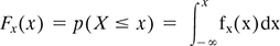
We will use the term cdf in this book to denote the distribution function or cumulative distribution function, which takes the form of random variable X as
Some of the important properties of Fx(x) are
5.4.1 Discrete random variables
Let us extend the concept of binary events by defining a discrete random variable X. Let X be a random variable with cdf Fx(x) and it changes values only in jumps (a countable number of them) and remains constant between the jumps then it is called a discrete random variable. So, the definition of a discrete random variable is that its range or the set X contains a finite or countably infinite number of points.
Let us consider that the jumps of Fx(x) of the discrete random variable X is occurring at points x1,x2,x3…., where this sequence represents a finite or countably infinite set and xi <xj if i < j. See Figure 5.2.
We can denote this through notation as
The probability of the event that X = x is denoted as p(X = x), or just p(x) for short. p is called a probability mass function (pmf).
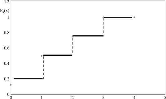
FIG. 5.2 A discrete random variable X with cdf Fx(x) = p(X ≤ x) for x = 0, 1, 2, 3, 4, and Fx(x) has jumps at x = 0, 1, 2, 3, 4
This satisfies the properties 0 ≤ p(x) ≤ 1 and Ʃx∈X p(x) = 1.
The cumulative distribution function (cdf) Fx(x) of a discrete random variable X can be denoted as
Refer to Figure 5.3, the pmf is defined on a finite state space X = {1, 2, 3, 4} that shows a uniform distribution with p(x ) = ![]() . This distribution means that X is always equal to the value
. This distribution means that X is always equal to the value ![]() , in other words, it is a constant.
, in other words, it is a constant.
Example. Suppose X is a discrete random variable with RX∈{0, 1, 2, …}. we can prove ![]() .
.
From the equation above,
Thus,
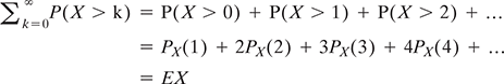
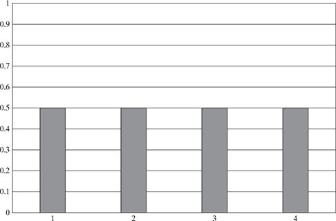
FIG. 5.3 A uniform distribution within the set {1, 2, 3, 4} where p(x = k) = ![]()
DISCUSSION POINTS
5.4.2 Continuous random variables
We have discussed the probabilities of uncertain discrete quantities. But most of the real-life events are continuous in nature. For example, if we have to measure the actual time taken to finish an activity then there can be an infinite number of possible ways to complete the activity and thus the measurement is continuous and not discrete as it is not similar to the discrete event of rolling a dice or flipping a coin. Here, the function Fx(x) describing the event is continuous and also has a derivative ![]() that exists and is piecewise continuous. The probability density function (pdf) of the continuous random variable x is defined as
that exists and is piecewise continuous. The probability density function (pdf) of the continuous random variable x is defined as
We will now see how to extend probability to reason about uncertain continuous quantities. The probability that x lies in any interval a ≤ x≤ b can be computed as follows.
We can define the events A = (x≤ a), B = (x≤ b), and W = (a < x≤ b). We have that B = A∪W, and since A and W are mutually exclusive, according to the sum rules:
Define the function F(q) = p(X ≤ q). The cumulative distribution function (cdf) of random variable X can be obtained by
which is a monotonically increasing function. Using this notation, we have
using the pdf of x, we can compute the probability of the continuous variable being in a finite interval as follows:
As the size of the interval gets smaller, it is possible to write
5.4.2.1 Mean and variance
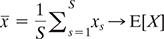
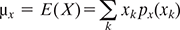
The mean in statistical terms represents the weighted average (often called as an expected value) of the all the possible values of random variable X and each value is weighted by its probability. It is denoted by µx or E(X) and defined as
mean is one of the important parameters for a probability distribution.
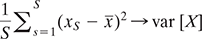
Variance of a random variable X measures the spread or dispersion of X. If E(X) is the mean of the random variable X, then the variance is given by
Points to Ponder:
The difference between Probability Density Function (pdf) and the Probability Mass Function (pmf) is that the latter is associated with the continuous random variable and the former is associated with the discrete random variable. While pmf represents the probability that a discrete random variable is exactly equal to some value, the pdf does not represent a probability by itself. The integration of pdf over a continuous interval yields the probability.
5.5 SOME COMMON DISCRETE DISTRIBUTIONS
In this section, we will discuss some commonly used parametric distributions defined on discrete state spaces, both finite and countably infinite.
5.5.1 Bernoulli distributions
When we have a situation where the outcome of a trial is withered ‘success’ or ‘failure’, then the behaviour of the random variable X can be represented by Bernoulli distribution. Such trials or experiments are termed as Bernoulli trials.
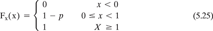
So we can derive that, a random variable X is called Bernoulli random variable with parameter p when its pmf takes the form of
Where 0 ≤ p ≤ 1. So, using the cdf Fx(x) of Bernoulli random variable is expressed as
The mean and variance of Bernoulli random variable X are
here, the probability of success is p and probability of failure is 1 – p. This is obviously just a special case of a Binomial distribution with n = 1 as we will discuss below.
5.5.2 Binomial distribution
If n independent Bernoulli trials are performed and X represents the number of success in those n trials, then X is called a binomial random variable. That’s the reason a Bernoulli random variable is a special case of binomial random variable with parameters (1, p).
The pmf of X with parameters (n, p) is given by
Where, 0 ≤ p ≤ 1 and
![]() is also called the binomial coefficient which is the number of ways to choose k items from n.
is also called the binomial coefficient which is the number of ways to choose k items from n.
For example, if we toss a coin n times. Let X ∈ {0, …, n} be the number of heads. If the probability of heads is p, then we say X has a binomial distribution, written as X ~Bin(n, p).
The corresponding cdf of x is
This distribution has the following mean and variance:
Figure 5.4 shows the binomial distribution of n = 6 and p = 0.6
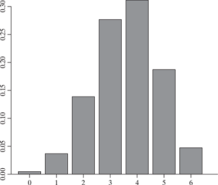
FIG. 5.4 A binomial distribution of n = 6 and p = 0.6
5.5.3 The multinomial and multinoulli distributions
The binomial distribution can be used to model the outcomes of coin tosses, or for experiments where the outcome can be either success or failure. But to model the outcomes of tossing a K-sided die, or for experiments where the outcome can be multiple, we can use the multinomial distribution. This is defined as: let x = (x1, …, xK) be a random vector, where xj is the number of times side j of the die occurs. Then x has the following pmf:
where, x1 + x2 +….. xK = n and
the multinomial coefficient is defined as
and the summation is over the set of all non-negative integers x1, x2, … . xk whose sum is n.
Now consider a special case of n = 1, which is like rolling a K-sided dice once, so x will be a vector of 0s and 1s (a bit vector), in which only one bit can be turned on. This means, if the dice shows up face k, then the k’th bit will be on. We can consider x as being a scalar categorical random variable with K states or values, and x is its dummy encoding with x = [Π(x = 1), …,Π(x = K)].
For example, if K = 3, this states that 1, 2, and 3 can be encoded as (1, 0, 0), (0, 1, 0), and (0, 0, 1). This is also called a one-hot encoding, as we interpret that only one of the K ‘wires’ is ‘hot’ or on. This very common special case is known as a categorical or discrete distribution and because of the analogy with the Binomial/ Bernoulli distinction, Gustavo Lacerda suggested that this is called the multinoulli distribution.
5.5.4 Poisson distribution
Poisson random variable has a wide range of application as it may be used as an approximation for binomial with parameter (n,p) when n is large and p is small and thus np is of moderate size. An example application area is, if a fax machine has a faulty transmission line, then the probability of receiving an erroneous digit within a certain page transmitted can be calculated using a Poisson random variable.
So, a random variable X is called a Poisson random variable with parameter λ (>0) when the pmf looks like
the cdf is given as:
Figure 5.5 shows the Poisson distribution with λ = 2
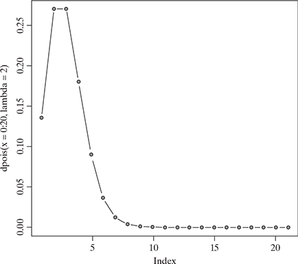
FIG. 5.5 A Poisson distribution with λ = 2
5.6 SOME COMMON CONTINUOUS DISTRIBUTIONS
In this section we present some commonly used univariate (one-dimensional) continuous probability distributions.
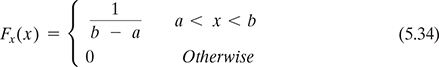
5.6.1 Uniform distribution
The pdf of a uniform random variable is given by:
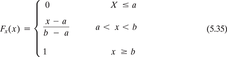
And the cdf of X is:
See Figure 5.6 that represents a uniform distribution with a = 3, b = 8 with increment 0.5 and repetition 20.
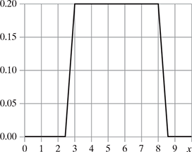
FIG. 5.6 A uniform distribution with a = 3, b = 8 with increment 0.5 and repetition 20
Example. If X is a continuous random variable with X~Uniform(a,b). Find E(X). We know as per equation 5.33
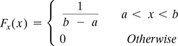
This is also corroborated by the fact that because X is uniformly distributed over the interval [a, b] we can expect the mean to be at the middle point, E(X) = ![]()
The mean and variance of a uniform random variable X are
This is a useful distribution when we don’t have any prior knowledge of the actual pdf and all continuous values in the same range seems to be equally likely.
5.6.2 Gaussian (normal) distribution
The most widely used distribution in statistics and machine learning is the Gaussian or normal distribution. Its pdf is given by
and the corresponding cdf looks like

For easier reference a function Φ(z) is defined as
Which will help us evaluate the value of Fx(x) which can be written as
It can be derived that
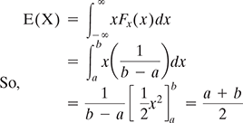
Figure 5.7 shows the normal distribution graph with mean = 4, s.d. = 12.
FIG. 5.7 A normal distribution graph
For a normal random variable, mean and variance are
the notation N(μ; σ2) is used to denote that p(X = x) = N(x|μ; σ2)
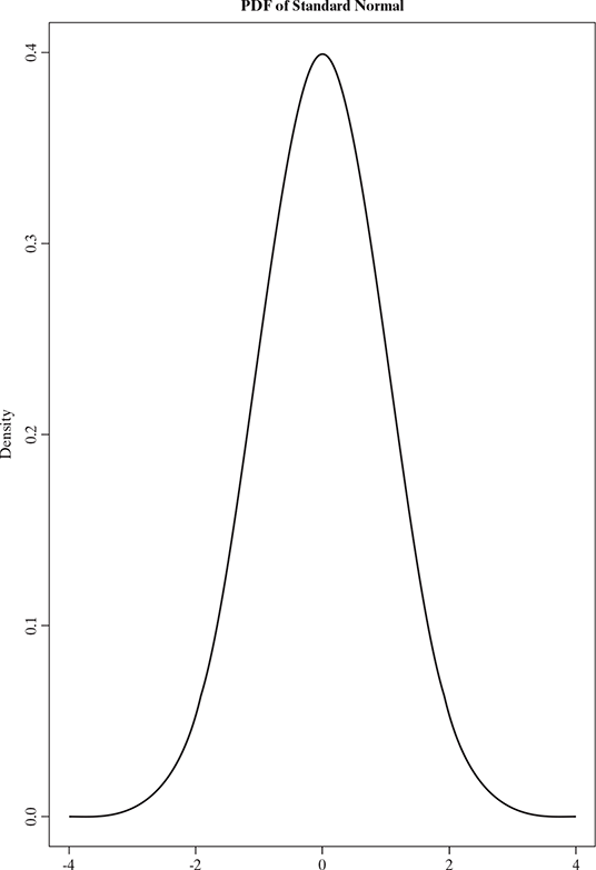
A standard normal random variable is defined as the one whose mean is 0 and variance is 1 which means Z = N(0;1). The plot for this is sometimes called the bell curve, (see Fig 5.8)
The Gaussian or Normal distribution is the most widely used distribution in the study of random phenomena in nature statistics due to few reasons:
- It has two parameters that are easy to interpret, and which capture some of the most basic properties of a distribution, namely its mean and variance.
- The central limit theorem ( Section 5.8) provides the result that sums of independent random variables have an approximately Gaussian distribution, which makes it a good choice for modelling residual errors or ‘noise’.
- The Gaussian distribution makes the least number of assumptions, subject to the constraint of having a specified mean and variance and thus is a good default choice in many cases.
- Its simple mathematical form is easy to implement, but often highly effective.
5.6.3 The laplace distribution
Another distribution with heavy tails is the Laplace distribution, which is also known as the double-sided exponential distribution. This has the following pdf:
Here μ is a location parameter and b >0 is a scale parameter.
Figure 5.9 represents the distribution of Laplace ![]()
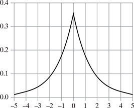
FIG. 5.9 The distribution graph of Laplace ![]()
This puts more probability density at 0 than the Gaussian. This property is a useful way to encourage sparsity in a model.
5.7 MULTIPLE RANDOM VARIABLES
Till now we were dealing with one random variable in a sample space, but in most of the practical purposes there are two or more random variables on the same sample space. We will discuss their associated distribution and interdependence.
5.7.1 Bivariate random variables
Let us consider two random variables X and Y in the sample space of S of a random experiment. Then the pair (X, Y) is called s bivariate random variable or two-dimensional random vector where each of X and Y are associated with a real number for every element of S. The range space of bivariate random variable (X, Y) is denoted by Rxy and (X, Y) can be considered as a function that to each point ζ in S assigns a point (x, y) in the plane.
(X, Y) is called a discrete bivariate random variable if the random variables X and Y both by themselves are discrete. Similarly, (X, Y) is called a continuous bivariate random variable if the random variables X and Y both are continuous and is called a mixed bivariate random variable if one of X and Y is discrete and the other is continuous.
5.7.2 Joint distribution functions
The joint cumulative distribution function (or joint cdf) of X and Y is defined as:
For the event (X ≤ x, Y ≤ y), we can define
A = {ζ∈S; X(ζ) ≤ x} and B = {ζ∈S; Y( ζ ) ≤ y}
And P(A) = FX(x) and P(B) = FY(y)
Then, FXY (x, y) = P (A ∩ B).
For certain values of x and y, if A and B are independent events of S, then
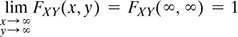
Few important properties of joint cdf of two random variables which are similar to that of the cdf of single random variable are
- 0 ≤ FXY (x, y) ≤ 1
If x1≤ x2 and y1≤ y2, then
FXY (x1, y1) ≤ FXY (x2, y1) ≤ FXY (x2, y2)
- FXY (x1, y1) ≤ FXY (x1, y2) ≤ FXY (x2, y2)


-
P (x1 < X ≤ x2, Y ≤ y) = FXY(x2, y)-FXY(x1, y)
P (X < x, y1 < Y ≤ y2) = FXY(x, y2)-FXY(x, y1)
5.7.3 Joint probability mass functions
For the discrete bivariate random variable (X, Y) if it takes the values (xi, yj) for certain allowable integers I and j, then the joint probability mass function (joint pmf) of (X, Y) is given by
Few important properties of pXY (xi, yj) are
- 0 ≤ pXY (xi, yj) ≤ 1
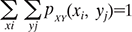
- P[(X, Y) ∈ A] = Ʃ (xi, yj) ∈ RA Ʃ pXY(xi, yj), where the summation is done over the points (xi, yj ) in the range space RA.
The joint cdf of a discrete bivariate random variable (X, Y) is given by
5.7.4 Joint probability density functions
In case (X, Y) is a continuous bivariate random variable with cdf FXY (x, y) and then the function,
is called the joint probability density function (joint pdf) of (X, Y). Thus, integrating, we get
Few important properties of fxy(x, y) are
- fxy(x, y) ≥ 0
5.7.5 Conditional distributions
While working with a discrete bivariate random variable, it is important to deduce the conditional probability function as X and Y are related in the finite space. Based on the joint pmf of (X, Y) the conditional pmf of Y when X = xi is defined as
Note few important properties of PY|X(yj|xi):
- 0 ≤ PY|X(yj|xi) ≤ 1
In the same way, when (X,Y) is a continuous bivariate random variable and has joint pdf fXY (x, y), then the conditional cdf of Y in case X = x is defined as
Note few important properties of fY|X(y|x):
- fY|X(y|x) ≥ 0
5.7.6 Covariance and correlation
The covariance between two random variables X and Y measure the degree to which X and Y are (linearly) related, which means how X varies with Y and vice versa.
So, if the variance is the measure of how a random variable varies with itself, then the covariance is the measure of how two random variables vary with each other.
Covariance can be between 0 and infinity. Sometimes, it is more convenient to work with a normalized measure, because covariance alone may not have enough information about the relationship among the random variables. For example, let’s define 3 different random variables based on flipping of a coin:
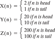
Just by looking into these random variables we can understand that they are essentially the same just a constant multiplied at their output. But the covariance of them will be very different when calculating with the equation 5.55:
To solve this problem, it is necessary to add a normalizing term that provides this intelligence: ![]()
If Cov (X,Y) = 0, then we can say X and Y are uncorrelated. Then from equation 5.55, X and Y are uncorrelated if
If X and Y are independent then it can be shown that they are uncorrelated, but note that the converse is not true in general.
So, we should remember
- The outcomes of a Random Variable weighted by their probability is Expectation, E(X).
- The difference between Expectation of a squared Random Variable and the Expectation of that Random Variable squared is Variance: E(X2) − E(X)2.
- Covariance, E(XY) − E(X)E(Y) is the same as Variance, but here two Random Variables are compared, rather than a single Random Variable against itself.
- Correlation, Corr (X, Y) =
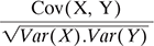 is the Covariance normalized.
Few important properties of correlation are
- −1 ≤ corr [X, Y] ≤ 1. Hence, in a correlation matrix, each entry on the diagonal is 1, and the other entries are between -1 and 1.
- corr [X, Y] = 1 if and only if Y = aX + b for some parameters a and b, i.e., if there is a linear relationship between X and Y.
- From property 2 it may seem that the correlation coefficient is related to the slope of the regression line, i.e., the coefficient a in the expression Y = aX + b. However, the regression coefficient is in fact given by a = cov[X, Y] /var [X]. A better way to interpret the correlation coefficient is as a degree of linearity.
5.8 CENTRAL LIMIT THEOREM
This is one of the most important theorems in probability theory. It states that if X1,… Xn is a sequence of independent identically distributed random variables and each having mean μ and variance σ2 and ![]()
As n → ∞ (meaning for a very large but finite set) then Zn tends to the standard normal.
Or
where, Φ(z) is the cdf of a standard normal random variable.
So, according to the central limit theorem, irrespective of the distribution of the individual Xi’s the distribution of the sum Sn – X1 + …Xn is approximately normal for large n. This is the very important result as whenever we need to deal with a random variable which is the sum of a large number of random variables than using central limit theorem we can assume that this sum is normally distributed.
5.9 SAMPLING DISTRIBUTIONS
As we discussed earlier in this chapter, an important application of statistics in machine learning is how to draw a conclusion about a set or population based on the probability model of random samples of the set. For example, based on the malignancy sample test results of some random tumour cases we want to estimate the proportion of all tumours which are malignant and thus advise the doctors on the requirement or non-requirement of biopsy on each tumour case. As we can understand, different random samples may give different estimates, if we can get some knowledge about the variability of all possible estimates derived from the random samples, then we should be able to arrive at reasonable conclusions. Some of the terminologies used in this section are defined below:
Population is a finite set of objects being investigated.
Random sample refers to a sample of objects drawn from a population in a way that every member of the population has the same chance of being chosen.
Sampling distribution refers to the probability distribution of a random variable defined in a space of random samples.
5.9.1 Sampling with replacement
While choosing the samples from the population if each object chosen is returned to the population before the next object is chosen, then it is called the sampling with replacement. In this case, repetitions are allowed. That means, if the sample size n is chosen from the population size of N, then the number of such samples is
Also, the probability of each sample being chosen is the same and is ![]() .
.
For example, let’s choose a random sample of 2 patients from a population of 3 patients {A, B, C} and replacement is allowed. There can be 9 such ordered pairs, like:
That means the number of random samples of 2 from the population of 3 is
and each of the random sample has probability ![]() of being chosen.
of being chosen.
5.9.2 Sampling without replacement
In case, we don’t return the object being chosen to the population before choosing the next object, then the random sample of size n is defined as the unordered subset of n objects from the population and called sampling without replacement. The number of such samples that can be drawn from the population size of N is
In our previous example, the unordered sample of 2 that can be created from the population of 3 patients when replacement is not allowed is
(A, B), (A, C), (B, C)
Also, each of these 3 samples of size 2 has the probability of getting chosen as ![]()
5.9.3 Mean and variance of sample
Let us consider X as a random variable with mean μ and standard deviation σ from a population N. A random sample of size n, drawn without replacement will generate n values x1, x2…..,xn for X. When samples are drawn with replacement, these values are independent of each other and can be considered as values of n independent random variables X1, X2,…., Xn, each having mean µ and variance σ2. The sample mean is a random variable Ẋ as
As X̅ is a random variable, it also has a mean µẋ and variance σẋ2 and it is related to population parameters as:
for a large number of n, if X is approximately normally distributed, then X̅ will also be normally distributed.
When the samples are drawn without replacement, then the sample values x1, x2…..,xn for random variable X are not independent. The sample mean X̅ has the mean µẊ and variance σẊ2 given by:
where, N is the size of the population and n < N. Also if X is normally distributed then X̅ also has a normal distribution.
Now, based on the central limit theorem, if the sample size of a random variable based on a finite population is large then the sample mean is approximately normally distributed irrespective of the distribution of the population. For most of the practical applications of sampling, when the sample size is large enough (as a rule of thumb ≥ 30) the sample mean is approximately normally distributed. Also, when a random sample is drawn from a large population, it can be assumed that the values x1, x2…..,xn are independent. This assumption of independence is one of the key to application of probability theory in statistical inference. We use the terms like ‘population is much larger than the sample size’ or ‘population is large compared to its sample size’, etc. to denote that the population is large enough to make the samples independent of each other. In practice, if ![]() , then independence may be assumed.
, then independence may be assumed.
5.10 HYPOTHESIS TESTING
While dealing with random variables a common situation is when we have to make certain decisions or choices based on the observations or data which are random in nature. The solutions for dealing with these situations is called decision theory or hypothesis testing and it is a widely used process in real life situations. As we discussed earlier, the key component of machine learning is to use a sample- based training data which can be used to represent the larger set of actual data and it is important to estimate how confidently an outcome can be related to the behaviour of the training data so that the decisions on the actual data can be made. So, hypothesis testing is an integral part of machine learning.
In terms of statistics, a hypothesis is an assumption about the probability law of the random variables. Take, e.g. a random sample (X1,….. Xn) of a random variable whose pdf on parameter κ is given by f(x, κ) = f(x1, x2…., xn; κ). We want to test the assumption κ = κ0 against the assumption κ = κ1. In this case, the assumption κ = κ0 is called null hypothesis and is denoted by H0. Assumption κ = κ1 is called alternate hypothesis and is denoted by H1.
A simple hypothesis is the one where all the parameters are specified with an exact value, like H0 or H1 in this case. But if the parameters don’t have an exact value, like H1:κ ≠ κ1 then H1 is composite.
Concept of hypothesis testing is the decision process used for validating a hypothesis. We can interpret a decision process by dividing an observation space, say R into two regions – R0 and R1. If x = (x1,…..xn) are the set of observation, then if x ∈ R0 the decision is in favor of H0and if x ∈ R1 then the decision is in favor of H1. The region R0is called acceptance region as the null hypothesis is accepted and R1 is the rejection region. There are 4 possible decisions based on the two regions in observation space:
- H0 is true; accept H0➔ this is a correct decision
- H0 is true; reject H0 (which means accept H1) ➔ this is an incorrect decision
- H1 is true; accept H1➔ this is a correct decision
- H1 is true; reject H1 (which means accept H0) ➔ this is an incorrect decision
So, we can see there is the possibility of 2 correct and 2 incorrect decisions and the corresponding actions. The erroneous decisions can be termed as:
Type I error: reject H0 (or accept H1) when H0 is true. The example of this situation is in a malignancy test of a tumour, a benign tumour is accepted as malignant tumour and corresponding treatment is started. This is also called Alpha error where good is interpreted as bad.
Type II error: reject H1 (or accept H0) when H1 is true. The example of this situation is in a malignancy test of a tumour, a malignant tumour is accepted as a benign tumour and no treatment for malignancy is started. This is also called Beta error where bad is interpreted as good and can have a more devastating impact.
The probabilities of Type I and Type II errors are
where, Di (I = 0, 1) denotes the event that the decision is for accepting Hi. PI is also denoted by α and known as level of significance whereas PII is denoted by β and is known as the power of the test. Here, α and β are not independent of each other as they represent the probabilities of the event from same decision problem. So, normally a decrease in one type of error leads to an increase in another type of when the sample size is fixed. Though it is desirable to reduce both types of errors it is only possible by increasing the sample size. In all practical applications of hypothesis testing, each of the four possible outcomes and courses of actions are associated with relative importance or certain cost and thus the final goal can be to reduce the overall cost.
So, the probabilities of correct decisions are
5.11 MONTE CARLO APPROXIMATION
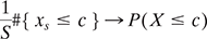
Though we discussed the distribution functions of the random variables, in practical situations it is difficult to compute them using the change of variables formula. Monte Carlo approximation provides a simple but powerful alternative to this. Let’s first generate S samples from the distribution, as x1, …, xS. For these samples, we can approximate the distribution of f(X) by using the empirical distribution of {f(xs)}Ss = 1.
In principle, Monte Carlo methods can be used to solve any problem which has a probabilistic interpretation. We know that by the law of large numbers, integrals described by the expected value of some random variable can be approximated by taking the empirical mean (or the sample mean) of independent samples of the random variable. A widely used sampler is Markov chain Monte Carlo (MCMC) sampler for parametrizing the probability distribution of a random variable. The main idea is to design a judicious Markov chain model with a prescribed stationary probability distribution. Monte Carlo techniques are now widely used in statistics and machine learning as well. Using the Monte Carlo technique, we can approximate the expected value of any function of a random variable by simply drawing samples from the population of the random variable, and then computing the arithmetic mean of the function applied to the samples, as follows:
This is also called Monte Carlo integration, and is easier to evaluate than the numerical integration which attempts to evaluate the function at a fixed grid of points. Monte Carlo evaluates the function only in places where there is a non-negligible probability.
For different functions f(), the approximation of some important quantities can be obtained:
- median{ x1, …, xs } → median(X)
5.12 SUMMARY
- Frequentist interpretation of probability represents the long run frequencies of events whereas the Bayesian interpretation of probability tries to quantify the uncertainty of some event and thus focuses on information rather than repeated trials.
- According to the Bayes rule, p (A|B) = p (B|A) p(A)/ p (B).
- A discrete random variable is expressed with the probability mass function (pmf) p(x) = p(X = x).
- A continuous random variable is expressed with the probability density function (pdf) p(x) = p(X = x).
- The cumulative distribution function (cdf) of random variable X can be obtained by
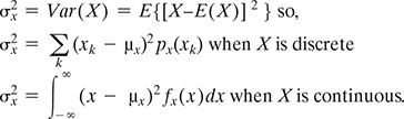
- The equation to find out the mean for random variable X is:
 when X is discrete
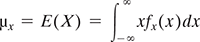 when X is continuous.
 - The equation to find out the variance for random variable X is
- When we have a situation where the outcome of a trial is withered ‘success’ or ‘failure’, then the behaviour of the random variable X can be represented by Bernoulli distribution.
- If n independent Bernoulli trials are performed and X represents the number of success in those n trials, then X is called a binomial random variable.
- To model the outcomes of tossing a K-sided die, or for experiments where the outcome can be multiple, we can use the multinomial distribution.
- The Poisson random variable has a wide range of application as it may be used as an approximation for binomial with parameter (n, p) when n is large and p is small and thus np is of moderate size.
- Uniform distribution, Gaussian (normal) distribution, Laplace distribution are examples for few important continuous random distributions.
- If there are two random variables X and Y in the sample space of S of a random experiment, then the pair (X, Y) is called as bivariate random variable.
- The covariance between two random variables X and Y measures the degree to which X and Y are (linearly) related.
- According to the central limit theorem, irrespective of the distribution of the individual Xi’s the distribution of the sum Sn – X1 + … Xn is approximately normal for large n.
- In hypothesis testing:
Type I error: reject H0 (or accept H1) when H0 is true.
Type II error: reject H1 (or accept H0) when H1 is true.
- Using the Monte Carlo technique, we can approximate the expected value of any function of a random variable by simply drawing samples from the population of the random variable, and then computing the arithmetic mean of the function applied to the samples.
SAMPLE QUESTIONS
MULTIPLE - CHOICE QUESTIONS (1 MARK EACH)
- The probabilistic approach used in machine learning is closely related to:
- Statistics
- Physics
- Mathematics
- Psychology
- This type of interpretation of probability tries to quantify the uncertainty of some event and thus focuses on information rather than repeated trials.
- Frequency interpretation of probability
- Gaussian interpretation of probability
- Machine learning interpretation of probability
- Bayesian interpretation of probability
- The reason the Bayesian interpretation can be used to model the uncertainty of events is that it does not expect the long run frequencies of the events to happen.
- True
- False
- p(A,B) = p(A ∩ B) = p(A|B) p(B) is referred as:
- Conditional probability
- Unconditional probability
- Bayes rule
- Product rule
- Based on this joint distribution on two events p(A,B), we can define the this distribution as follows:
- p(A) = p(A,B) = p(A|B = b) p(B = b)
- Conditional distribution
- Marginal distribution
- Bayes distribution
- Normal distribution
- We can define this probability as p(A|B) = p(A,B)/p(B) if p(B) > 0
- Conditional probability
- Marginal probability
- Bayes probability
- Normal probability
- In statistical terms, this represents the weighted average score.
- Variance
- Mean
- Median
- More
- The covariance between two random variables X and Y measures the degree to which X and Y are (linearly) related, which means how X varies with Y and vice versa. What is the formula for Cov (X,Y)?
- Cov(X,Y) = E(XY)−E(X)E(Y)
- Cov(X,Y) = E(XY)+ E(X)E(Y)
- Cov(X,Y) = E(XY)/E(X)E(Y)
- Cov(X,Y) = E(X)E(Y)/ E(XY)
- The binomial distribution can be used to model the outcomes of coin tosses.
- True
- False
- Two events A and B are called mutually exclusive if they can happen together.
- True
- False
SHORT-ANSWER TYPE QUESTIONS (5 MARKS EACH)
- Define the Bayesian interpretation of probability.
- Define probability of a union of two events with equation.
- What is joint probability? What is its formula?
- What is chain rule of probability?
- What is conditional probability means? What is the formula of it?
- What are continuous random variables?
- What are Bernoulli distributions? What is the formula of it?
- What is binomial distribution? What is the formula?
- What is Poisson distribution? What is the formula?
- Define covariance.
- Define correlation
- Define sampling with replacement. Give example.
- What is sampling without replacement? Give example.
- What is hypothesis? Give example.
LONG-ANSWER TYPE QUESTIONS (10 MARKS QUESTIONS)
- Let X be a discrete random variable with the following PMF
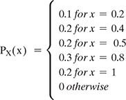
- Find the range RX of the random variable X.
- Find P(X ≤ 0.5)
- Find P(0.25<X<0.75)
- Find P(X = 0.2|X<0.6)
- Two equal and fair dice are rolled and we observed two numbers X and Y.
- Find RX, RY and the PMFs of X and Y.
- Find P(X = 2,Y = 6).
- Find P(X>3|Y = 2).
- If Z = X + Y. Find the range and PMF of Z.
- Find P(X = 4|Z = 8).
- In an exam, there were 20 multiple-choice questions. Each question had 44 possible options. A student knew the answer to 10 questions, but the other 10 questions were unknown to him and he chose answers randomly. If the score of the student X is equal to the total number of correct answers, then find out the PMF of X. What is P(X>15)?
- The number of students arriving at a college between a time interval is a Poisson random variable. On an average 10 students arrive per hour. Let X be the number of students arriving from 10 am to 11:30 am. What is P(10<X≤15)?
- If we have two independent random variables X and Y such that X~Poisson(α) and Y~Poisson(β). Define a new random variable as Z = X + Y. Find out the PMF of Z.
- There is a discrete random variable X with the pmf.
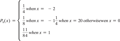
If we define a new random variable Y = (X + 1)2 then
- Find the range of Y.
- Find the pmf of Y.
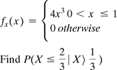
- If X is a continuous random variable with PDF
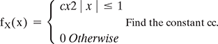
- Find EX and Var(X).
- Find P(X ≥
 ).
).
- If X is a continuous random variable with pdf
- If X~Uniform
 and Y = sin(X), then find fY(y).
 - If X is a random variable with CDF
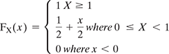
- What kind of random variable is X: discrete, continuous, or mixed?
- Find the PDF of X, fX(x).
- Find E(eX).
- Find P(X = 0|X≤0.5).
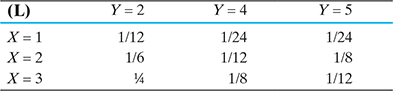
- There are two random variables X and Y with joint PMF given in Table below
- Find P(X≤2, Y≤4).
- Find the marginal PMFs of X and Y.
- Find P(Y = 2|X = 1).
- Are X and Y independent?
- There is a box containing 40 white shirts and 60 black shirts. If we choose 10 shirts (without replacement) at random, then find the joint PMF of X and Y where X is the number of white shirts and Y is the number of black shirts.
- If X and Y are two jointly continuous random variables with joint PDF
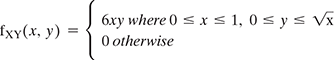
- Find fX(x) and fY(y).
- Are X and Y independent to each other?
- Find the conditional PDF of X given Y = y, fX|Y(x|y).
- Find E[X|Y = y], for 0 ≤ y ≤ 1.
- Find Var(X|Y = y), for 0 ≤ y ≤ 1.
- There are 100 men on a ship. If Xi is the weight of the ith man on the ship and Xi’s are independent and identically distributed and also EXi = μ = 170 and σXi = σ = 30. Find the probability that the total weight of the men on the ship exceeds 18,000.
- Let X1, X2, ……, X25 are the independent and identically distributed. And have the following PMF
If Y = X1 + X2 + … + Xn, estimate P(4 ≤ Y ≤ 6) using central limit theorem.